Lasso formulation of the shortest path problem

Anqi Dong Amirhossein Taghvaei Tryphon T. Georgiou Thanks: A. Dong, A. Taghvaei, and T. T. Georgiou are with the Department of Mechanical and Aerospace Engineering, University of California, Irvine, CA 92697-3975; {anqid2,ataghvae,tryphon}@uci.edu

Abstract

The shortest path problem is formulated as an $l_{1}$ -regularized regression problem, known as lasso. Based on this formulation, a connection is established between Dijkstra’s shortest path algorithm and the least angle regression (LARS) for the lasso problem. Specifically, the solution path of the lasso problem, obtained by varying the regularization parameter from infinity to zero (the regularization path), corresponds to shortest path trees that appear in the bi-directional Dijkstra algorithm. Although Dijkstra’s algorithm and the LARS formulation provide exact solutions, they become impractical when the size of the graph is exceedingly large. To overcome this issue, the alternating direction method of multipliers (ADMM) is proposed to solve the lasso formulation. The resulting algorithm produces good and fast approximations of the shortest path by sacrificing exactness that may not be absolutely essential in many applications. Numerical experiments are provided to illustrate the performance of the proposed approach.

I Introduction

The problem of finding the shortest path between two vertices in a graph has a long history [1],[2] with a wide range of applications Waxman [3] Mortensen et al. [4]. The classical algorithm to determine a shortest path is due to Edsger W. Dijkstra [5]. Since Dijkstra’s early work, a variety of alternative methods to identify a shortest path have been developed to reduce complexity and improve speed [6, 7, 8, 9]. However, it is often the case that finding a shortest path is not absolutely essential, especially in graphs of considerably large sizes, while a reasonably short path may suffice [3, 10]. Motivated by such considerations and inspired by success of convex optimization to address large-scale problems [11, 12], we introduce a formulation of the shortest path problem as an $l_{1}$ -regularized regression, known as the “lasso” (Least Absolute Shrinkage and Selection Operator) problem [13].

Specifically, in this paper, we discuss two novel and important implications of the lasso formulation which constitute our main contributions.

(i) We provide a rather surprising connection between Dijkstra’s algorithm and the solution path of the lasso problem; we show that the solution path of the lasso problem generates shortest path trees that appear in Dijkstra’s algorithm. The connection is interesting as the lasso solution path is based on analytical arguments, invoking KKT conditions, unlike the Dijkstra’s algorithm that is akin to Dynamic Programming, cf. Figure 1.

(ii) On the practical side, we consider the shortest path problem on graphs with large size and propose to utilize the ADMM method to obtain approximate shortest path solutions. Moreover, the ADMM method can be implemented in a distributed manner, and has the flexibility to be initialized with a rough approximation of the shortest path (if one such is available) for faster convergence; this option arise in cases where a graph undergoes slight variation from an earlier one where a short path is available, cf. Figure 3(b) and Figure 5(a)

Refer to caption — (a) Step $0$ : $\lambda_{0}=\infty$

Here is the outline of the paper: The necessary preliminary definitions and notations are introduced in Section II. The Lasso formulation is presented in Section III. The analysis of solution path of the lasso appears in Section IV. The connection with Dijkstra’s algorithm appears in Section V. The ADMM algorithm and its application to shortest path problem to large graphs is presented in Section VI.

II Preliminaries

II-A Graph theoretic notations and definitions

Consider a weighted undirected graph $\mathcal{G}=(\mathcal{V},\mathcal{E},\mathcal{W})$ with vertex set $\mathcal{V}=\{1,\dots,n\}$ and a set of edges $\mathcal{E}=\{e_{1},\dots,e_{m}\}$ with corresponding positive weights in $\mathcal{W}=\{w_{1},\ldots,w_{m}\}$ . The graph is assumed to be connected and simple (i.e., with no self-loops or multi-edges). The edge that connects the nodes $i$ and $j$ is also denoted by the pair of nodes as $(i,j)$ . Although the graph is undirected, we assign an arbitrary but fixed orientation to each edge.

The incidence matrix of the graph, denoted by $D$ , is a $n\times m$ matrix whose $(i,j)$ -th entry is defined according to

[D]_{ij}=\begin{cases}+1\ \ \ &\text{if vertex $i$ is at the tail of edge $e_{j}$},\\ -1\ \ \ &\text{if vertex $i$ is at the head of edge $e_{j}$},\\ 0\ \ \ &\text{otherwise}.\end{cases}

The graph Laplacian matrix, denoted by $L$ , is a $n\times n$ matrix defined as

\displaystyle L=DWD^{T}

where $W=\text{diag}(w_{1},\ldots,w_{m})$ is the diagonal matrix formed by the weights.

A path from vertex $s$ to vertex $t$ is a sequence of connected edges $p=\{(v_{0},v_{1}),(v_{1},v_{2}),\ldots,(v_{l-1},v_{l})\}\subset\mathcal{E}$ that originates at $v_{0}=s$ and ends at $v_{l}=t$ . The incidence vector $x^{(p)}$ of a path $p$ is $m$ -dimensional vector defined as follows. The $i$ -th entry of $x^{(p)}$ is zero, if the path does not contain the edge $e_{i}$ . If the path contains $e_{i}$ , then the corresponding entry is either $+1$ or $-1$ . The sign is positive/negative depending on whether the direction of the path agrees/disagrees with direction of the edge. The length of the path is the sum of the weights of the edges that belong to the path, i.e.,

\text{length}(p)\triangleq\sum_{e_{i}\in p}w_{i}=\|Wx^{(p)}\|_{1}

where $\|\cdot\|_{1}$ denotes the $l_{1}$ -norm.

Definition II.1.

When $\mathcal{G}$ is a tree with root at vertex $1$ , the path matrix $P$ is defined to be the $(n-1)\times(n-1)$ matrix whose $i$ -th column is the incidence vector of the path from vertex $i$ to the root $1$ , for $i=2,3,\ldots,n$ .

The pseudo-inverse of the incidence matrix of a tree admits a simple representation in terms of the path matrix [14, Theorem 2.10, Lemma 2.15].

Lemma II.1.

Let $D$ be the incidence matrix of a tree with vertices $\mathcal{V}=\{1,2,\ldots,n\}$ and root vertex $1$ . Then, the pseudo-inverse of $D$ is given by

D^{+}=\begin{bmatrix}-\frac{1}{n}P\mathbbm{1}&PJ\end{bmatrix}_{(n-1)\times n}

(1)

where

\mathbbm{1}:=[1,1,\ldots,1]^{T}_{n-1}

is $(n-1)$ -dimensional (column) vector of ones,

J=(I-\frac{1}{n}\mathbbm{1}\mathbbm{1}^{T})

is an orthogonal projection with null space spanned by $\mathbbm{1}$ , $I$ is identity matrix of size $(n-1)\times(n-1)$ , and $P$ is the $(n-1)\times(n-1)$ path matrix of the tree, defined in II.1.

II-B Shortest path problem

Let $\mathcal{P}_{s,t}$ denote the set of all paths between $s$ and $t$ . This set is non-empty because the graph is connected. The shortest path problem is to find a path between $s$ and $t$ with minimum length, mathematically formulated as finding

{\rm arg}\min_{p\in\mathcal{P}_{s,t}}~\text{length}(p).

(2)

The minimum value is the distance between $s$ and $t$ , and the minimizing path is the shortest path between $s$ and $t$ .

II-C Dijkstra’s algorithm

Dijkstra’s algorithm to find the shortest path from $v_{s}$ to $v_{t}$ involves the following variables:

•

dist: an array of distances from the root vertex $v_{s}$ to all the other vertices in the graph.
•

$\mathcal{S}$ : the set of visited vertices.
•

$\mathcal{Q}$ : the queue of vertices to be visited.

The algorithm begins with initial $\infty$ values for the distances and improve the distance step by step as follows

Algorithm 1 Dijkstra’s algorithm

0: source vertex

v_{s}

and target vertex

v_{t}

0: the shortest path and the length of the path.

dist^{(0)}

[

v_{s}

]

=0

dist^{(0)}

[

v_{i}

]

=\infty,\forall v_{i}\neq v_{s}

\mathcal{S}=\emptyset

\mathcal{Q}=\mathcal{V}

2: while

v_{t}\notin S

3: pick

u

from

Q

with minimum distance:

u=\argmin\limits_{v\in Q}dist[v]

4: Remove

u

from

Q

Q\leftarrow Q\setminus\{u\}

5: Add

u

S

S\leftarrow S\cup\{u\}

6: for

v_{i}\in\textit{neighbors}[u]

7: if dist[

v_{i}

]

>

dist[

u

]

+w_{u,v_{i}}

then

\textit{dist}[v_{i}]\leftarrow\textit{dist}[u]+w_{u,v_{i}}

9: end if

10: end for

11: end while

12: return dist[

v_{t}

]

The essential feature of the Dijkstra’s algorithm is that, the algorithm iteratively constructs the shortest path tree that is rooted at $s$ , to all the visited vertices before reaching the target $t$ . Later in Section V, we show that such a feature is also observed in the Lasso formulation of the shortest path problem.

III Lasso formulation of the shortest path problem

III-A Linear programming formulation

The shortest path problem (2) can be formulated as a linear programming problem on the incidence vectors. The condition that a path, or in general a collection of edges, forms a path between $s$ and $t$ can be expressed as a linear constraint on the incidence vector:

p\in\mathcal{P}_{s,t}\quad\Rightarrow\quad Dx^{(p)}=y^{(s,t)}

(3)

where $y^{(s,t)}\in\mathbb{R}^{n}$ is defined according to

\displaystyle y^{(s,t)}(i)=\begin{cases}+1,&\text{if}\ i=s,\\ -1,&\text{if}\ i=t,\\ 0,&\text{otherwise}.\end{cases}\ \ \ 1\leq i\leq n

The justification for (3) is straightforward. For any two connecting edges $e_{i}=(v_{1},v_{2})$ and $e_{j}=(v_{2},v_{3})$ , the summation of the $i$ -th and $j$ -th columns of $D$ is equal to $y^{(v_{1},v_{3})}$ , which corresponds to the edge $(v_{1},v_{3})$ . Likewise, an additional column corresponding to the edge $(v_{3},v_{4})$ , yields $y^{(v_{1},v_{4})}$ . Therefore, $Dx^{(p)}$ , results in the summation of all columns corresponding to a set of connecting edges $p=\{(s,v_{1}),(v_{1},v_{2}),\ldots,(v_{l-1},t)\}$ , and this is $y^{(s,t)}$ .

Remark III.1.

An alternative justification can be provided by noting that closed cycles, i.e., paths that begin and end at the same node, form a basis for the null space of the incidence matrix of the graph [14, 15]. If we attach a virtual direct link (i.e., a new edge) between vertices $s$ and $t$ , we need to update the incidence matrix to $\left[\begin{matrix}D&-y^{(s,t)}\end{matrix}\right]$ so that this virtual edge is included. Now a path from $s$ to $t$ “closes” into a cycle by including this extra virtual edge. Any cycle that includes the virtual edge corresponds to a null vector of $\left[\begin{matrix}D&-y^{(s,t)}\end{matrix}\right]$ with a $1$ as the last entry (indicating that the virtual edge is included), and therefore, to a solution of

\left[\begin{matrix}D&-y^{(s,t)}\end{matrix}\right]\left[\begin{matrix}x^{(p)}\\ 1\end{matrix}\right]=0.

This is precisely (3), while the first component $x^{(p)}$ of the solution vector corresponds to a sought path from $s$ to $t$ .

Evidently, the conclusion (3) does hold in the reverse direction: vectors that satisfy the linear constraint $Dx^{(p)}=y^{(s,t)}$ may take fractional values and do not correspond to a valid incidence vector. For instance, any linear combination $x=ax^{(p_{1})}+(1-a)x^{(p_{2})}$ for $a\in[0,1]$ of the incidence vectors $x^{(p_{1})}$ and $x^{(p_{2})}$ of two distinct paths, $p_{1}$ and $p_{2}$ , between $s$ and $t$ , satisfies the constraint $Dx=y^{(s,t)}$ . Yet, if the shortest path is unique, then a solution to (3) with the least number of nonzero entries would necessarily correspond to this shortest path. Thus, although the exact equivalency does not hold for (3), the shortest path can be recovered from the “sparsest” solution to (3).

Now, a well known fact, that underlies techniques in modern compressive sensing [13], is that the $\ell_{1}$ norm can be used as a suitable surrogate for obtaining “sparse” solutions. Thus, we propose as a relaxation to the shortest path problem the following:

{\rm arg}\min_{x\in\mathbb{R}^{m}}~\|Wx\|_{1},\quad\text{s.t.}\quad Dx=y^{(s,t)}

(4)

This is a linear programming problem and, for the reasons just noted, if the shortest path is unique, then the solution turns out to be integer-valued and corresponding to a valid incidence vector [16, Theorem 6.5 (Integrality Theorem), p. 186].

III-B Lasso formulation

It is natural to consider the following $l_{1}$ -regularized regression problem by replacing the constraint with a penalty term and changing variables by introducing $\beta=Wx$ :

\min_{\beta\in\mathbb{R}^{m}}~\frac{1}{2}\|y-Q\beta\|_{2}^{2}+\lambda\|\beta\|_{1}.

(5)

Here $\lambda>0$ is the regularization parameter and $Q\triangleq DW^{-1}$ . Problem (5) is known as the lasso problem. For $\lambda>0$ , the solution of (5) is no longer equal to the shortest path. However, in the limit as $\lambda\to 0$ , the solution becomes exact. Our motivation for exploring the formulation (5) is twofold:
(i) As shown in Section IV, the LARS algorithm, designed to solve the lasso problem (5), is equivalent to Dijkstra’s algorithm, and
(ii) as discussed in Section VI, it allows the flexibility to us proximal optimization methods to obtain a good approximation of the shortest path in large graph setting.

III-C Uniqueness of the Lasso solution

The solution to the Lasso problem is unique when $\text{rank}(D)=m$ , i.e. the rank of incidence matrix is equal to the number of edges. This condition holds if only if the graph is a tree (or a collection of disjoint trees). Evidently, the assumption that the graph is a tree is too restrictive, especially for the shortest path problem, because the problem becomes trivial.

The rank condition $\text{rank}(D)=m$ is sufficient but not necessary. Relaxations of this assumption have been introduced in the literature [17]. We use the result [17, lemma 2] to prove the uniqueness of the lasso solution under the following assumption.

Assumption A1: The shortest path between vertex $s$ or $t$ and any other vertex is unique.

The uniqueness result is expressed in the following lemma. The proof appears in Appendix -C.

Lemma III.2.

Under assumption A1, the lasso problem (5) admits a unique solution for all $\lambda>0$ .

Remark III.3.

Assumption A1 is satisfied for a generic selection of weights, for example if a small noise is added to the weights. The assumption is necessary, as it is straightforward to come up with counter examples.

IV Solution path and LARS algorithm

IV-A KKT conditions

Let $\beta(\lambda)$ denote the solution to the lasso problem (5). It must satisfy the KKT condition,

\displaystyle Q^{T}(y-Q\beta(\lambda))=\lambda\gamma,

(6)

where $\gamma$ belongs to sub-differential of $\|\beta(\lambda)\|_{1}$ whose $j$ -th component is given by

\displaystyle\gamma_{j}\in\begin{cases}\{\text{sign}(\beta_{j}(\lambda))\}~~&\text{if}\;\beta_{j}(\lambda)\neq 0\\ \left[-1,1\right]~~&\text{if}\;\beta_{j}(\lambda)=0.\end{cases}

(7)

The KKT condition motivates to divide the indices $\{1,\ 2,\dots,m\}$ into two sets: active set $\mathcal{A}$ , where $\beta(\lambda)$ is nonzero, and non-active set $\mathcal{A}^{c}$ , where $\beta(\lambda)$ is zero. Let $\beta_{\mathcal{A}}(\lambda)$ denote the vector $\beta(\lambda)$ where non-active components are removed, and $Q_{\mathcal{A}}$ be the matrix $Q$ where the columns corresponding to non-active set are removed. Then, the KKT condition (6) is expressed as


$\displaystyle Q_{j}^{T}(y-Q_{\mathcal{A}}\beta_{\mathcal{A}}(\lambda))$	$\displaystyle=s_{j}\lambda,\quad\forall j\in\mathcal{A}$	(8a)
$\displaystyle Q_{j}^{T}(y-Q_{\mathcal{A}}\beta_{\mathcal{A}}(\lambda))$	$\displaystyle\in[-\lambda,\lambda],\quad\forall j\in\mathcal{A}^{c},$	(8b)

where $Q_{j}$ denotes the $j$ -th column of $Q$ and the sign vector

s\triangleq\text{sign}\left(Q_{\mathcal{A}}^{T}(y-Q_{\mathcal{A}}\beta_{\mathcal{A}}(\lambda))\right)=\text{sign}\left(\beta_{\mathcal{A}}\right).

(9)

IV-B LARS algorithm

The least angle regression (LARS) algorithm, in its lasso state¹¹ 1 Whereas the original LARS algorithm does not provide the lasso solution, a modification in [18] does indeed solve the lasso problem., finds the solution $\beta(\lambda)$ that satisfy the KKT condition (8) for all $\lambda>0$ [18]. The vector $\beta(\lambda)$ is continuous and piecewise linear, as a function of $\lambda$ , with break points $\lambda_{1}>\lambda_{2}>\ldots>\lambda_{l}>0$ . The active set and the sign vector remain the same during each interval and change at each break points. Let $\mathcal{A}_{k}$ and $s_{k}$ denote the active set and sign vector during the interval $(\lambda_{k+1},\lambda_{k})$ . The LARS algorithm starts with $\lambda_{0}=\infty$ , $\mathcal{A}_{0}=\emptyset$ , and $s_{0}=\emptyset$ . Then, at iteration $k$ , given $\lambda_{k}$ , $\mathcal{A}_{k}$ , and $s_{k}$ , the algorithm finds the next breaking point $\lambda_{k+1}$ , the next active set $\mathcal{A}_{k+1}$ , and the next sign vector $s_{k+1}$ . During each interval $(\lambda_{k+1},\lambda_{k})$ , the vector $\beta(\lambda)$ is the minimum $l_{2}$ -norm solution of the condition (8a) given by:

	$\displaystyle\beta_{\mathcal{A}_{k}}(\lambda)$	$\displaystyle=(Q_{\mathcal{A}_{k}}^{T}Q_{\mathcal{A}_{k}})^{+}(Q_{\mathcal{A}_{k}}^{T}y-\lambda s_{k})$		(10)
		$\displaystyle=a^{(k)}-b^{(k)}\lambda,$

where ⁺ denotes the Moore-Penrose pseudo-inverse and


$\displaystyle a^{(k)}$	$\displaystyle\triangleq(Q_{\mathcal{A}_{k}}^{T}Q_{\mathcal{A}_{k}})^{+}Q_{\mathcal{A}_{k}}^{T}y,$	(11a)
$\displaystyle b^{(k)}$	$\displaystyle\triangleq(Q_{\mathcal{A}_{k}}^{T}Q_{\mathcal{A}_{k}})^{+}s_{k}.$	(11b)

The next breaking point $\lambda_{k+1}$ is the largest value $\lambda<\lambda_{k}$ so that (10) does not satisfy the KKT conditions (8) anymore. The KKT conditions are violated in two cases:

•

Joining: This case happens when condition (8b) is violated for some $j\in\mathcal{A}^{c}_{k}$ , i.e. $|Q_{j}^{T}(y-Q_{\mathcal{A}_{k}}\beta_{\mathcal{A}_{k}}(\lambda))|=\lambda$ . For each index $j\in\mathcal{A}^{c}_{k}$ , this happens at $\lambda=t^{\text{join}}_{j}$ given by

$t^{\text{join}}_{j,k}=\frac{Q_{j}^{T}(Q_{\mathcal{A}_{k}}a^{(k)}-y)}{Q_{j}^{T}Q_{\mathcal{A}_{k}}b^{(k)}\pm 1}.$ (12)

•

Crossing: This case happens when condition (8a) is violated for some $j\in\mathcal{A}_{k}$ . By definition of $\beta_{\mathcal{A}_{k}}(\lambda)$ according to (10), the condition (8a) is violated only when $s\neq s_{k}$ . This happens when one of the component of $\beta_{\mathcal{A}_{k}}(\lambda)$ crosses zero, i.e. $a^{(k)}_{j}-\lambda b^{(k)}_{j}=0$ for some $\lambda<\lambda_{k}$ . For each index $j\in\mathcal{A}_{k}$ , the crossing happens at $\lambda=t^{\text{cross}}_{j}$ given by

t_{j,k}^{\text{cross}}=\begin{cases}\frac{a^{(k)}_{j}}{b^{(k)}_{j}}\quad&\text{if}~0<\frac{a^{(k)}_{j}}{b^{(k)}_{j}}<\lambda_{k}\\ 0\quad&\text{otherwise}.\end{cases}

(13)

The algorithm selects the next break point $\lambda_{k+1}$ to be the maximum of joining times and crossing times:

\lambda_{k+1}=\max(\max_{j\in\mathcal{A}_{k}^{c}}t^{\text{join}}_{j,k},\max_{j\in\mathcal{A}_{k}}t_{j,k}^{\text{cross}})

(14)

If the joining happens, the joining index is added to the active set and the sign vector is updated accordingly. If a crossing happens, the crossing index is removed from the active set. The overall algorithm is summarized in 2.

Algorithm 2 LARS path algorithm for the lasso problem (5)

0: matrix

Q=DW^{-1}

and vector

y=y^{(s,t)}

0: incidence vector

x=W^{-1}\beta

and path length

\|\beta\|_{1}

k=0

\lambda_{0}=\infty

\mathcal{A}=\emptyset

s=0

a^{(0)}=0

and

b^{(0)}=0

2: while

\lambda_{k}>0

3: Compute the joining time (12) for

j\in\mathcal{A}^{c}_{k}

4: Compute the crossing time (13) for

j\in\mathcal{A}_{k}

5: Set

\lambda_{k+1}

according to (14)

•

If join happens, add the joining index to $\mathcal{A}_{k}$ and its sign to $s_{k}$ .
•

If cross happens, remove the crossing index from $\mathcal{A}_{k}$ and its sign from $s_{k}$ .

k=k+1

7: Compute

a^{(k)}

and

b^{(k)}

according to (11)

8: Set

\beta_{\mathcal{A}_{k}}=a^{(k)}-\lambda_{k}b^{(k)}

and

\beta_{\mathcal{A}_{k}^{c}}=0

9: end while

10: return

x=W^{-1}\beta

and

\|\beta\|_{1}

IV-C Numerical example

Consider the Nicholson’s graph [19, p. 6], as depicted in Figure 1(a), and the shortest path problem between vertex $1$ and vertex $9$ . The iterations of the LARS algorithm are depicted in Figure 1. At each iteration, the edges that belong to the active set $\mathcal{A}$ are highlighted in red. It is observed that at each iterations, edges are added to the active set and are never removed. The algorithm terminates after four iterations when $\lambda_{5}=0$ and a path between vertex $1$ and $9$ is formed. The lasso solution path $\beta(\lambda)$ is depicted in Figure 1(g).

Example 1 illustrates the similarity between LARS algorithm and the Dijkstra’s algorithm. Namely, the LARS algorithm constructs two shortest-path trees, with roots at vertex $1$ and vertex $9$ respectively. This is similar to the bi-directional Dijkstra’s algorithm, as discussed in Section II. In the next section, we show that the similarity between the LARS algorithm and the Dijkstra’s algorithm holds in general.

V Relationship between LASSO and Dijkstra

We establish the connection between the LARS algorithm 2 and the Dijkstra’s algorithm by showing that the LARS algorithm iteratively builds two shortest path trees with roots at $s$ and $t$ , and that the algorithm terminates when the two trees connect.

We prove this by induction. The induction hypothesis is as follows: At iteration $k$ of the algorithm, the edges in the active set $\mathcal{A}_{k}=\mathcal{A}_{k}^{(s)}\cup\mathcal{A}_{k}^{(t)}$ form two disjoint subsets $\mathcal{A}_{k}^{(s)}$ and $\mathcal{A}_{k}^{(s)}$ . Each subset form a tree on the vertices, denoted by $T^{(s)}_{k}\subset\mathcal{V}$ with root at $s$ and $T^{(t)}_{k}\subset\mathcal{V}$ with root at $t$ , respectively. The two trees are the shortest-path trees from the root vertex. Moreover, crossing does not occur at this iteration, i.e., no edges are removed from the active set.

The induction hypothesis is true at $k=0$ , because the active set is empty, the two trees consist of single root vertex, i.e. $T^{(s)}_{0}=\{s\}$ and $T^{(t)}_{0}=\{t\}$ , and crossing does not occur because the active set is empty.

Assuming the induction hypothesis at iteration $k$ , we show the hypothesis also holds at iteration $k+1$ by proving:

(a)

Let $v_{\text{min}}^{(s)}$ and $v_{\text{min}}^{(t)}$ denote the vertex that has the minimum distance to the root $s$ and $t$ respectively, among all vertices outside the two trees. Then, either the edge that connects vertex $v_{\text{min}}^{(s)}$ to tree $T^{(s)}_{k}$ or the edge that connects $v_{\text{min}}^{(t)}$ to $T^{(t)}_{k}$ is added to the active set;
(b)

Crossing does not occur.

Moreover, we also need to show the termination condition

The proof is based on simplified expressions for joining time and the crossing time that are obtained using Lemma II.1. The derivations appear in Appendix -A and -B.

V-1 Joining time

For the edge $e_{j}=(v_{1},v_{2})$ , where $e_{j}\in\mathcal{A}_{k}^{c}$ , the joining time is

\displaystyle t^{\text{join}}_{j,k}=\begin{cases}0~&\text{if}~(v_{1},v_{2})\in\Omega^{2}\\ 0~&\text{if}~(v_{1},v_{2})\in{T^{(s)}_{k}}^{2}\cup{T^{(t)}_{k}}^{2}\\ \frac{1}{|T^{(s)}_{k}|l^{(s)}_{v_{2}}-\sum_{v\in T^{(s)}_{k}}l^{(s)}_{v}}~&\text{if}~(v_{1},v_{2})\in{T^{(s)}_{k}}\times\Omega\\ \frac{1}{|T^{(t)}_{k}|l^{(s)}_{v_{2}}-\sum_{v\in T^{(t)}_{k}}l^{(t)}_{v}}~&\text{if}~(v_{1},v_{2})\in{T^{(t)}_{k}}\times\Omega\\ \frac{|T^{(s)}_{k}|+|T^{(t)}_{k}|}{\gamma}~&\text{if}~(v_{1},v_{2})\in{T^{(s)}_{k}}\times{T^{(t)}_{k}}\end{cases}

(15)

where $\Omega$ is the set of vertices not in the trees, $l^{(s)}_{v}$ and $l^{(t)}_{v}$ denote the distance of vertex $v$ to the root $s$ and $t$ respectively, and

\gamma=|T^{(s)}_{k}||T^{(t)}_{k}|l^{(s)}_{t}-|T^{(t)}_{k}|\sum_{v\in T^{(s)}_{k}}l_{v}^{(s)}-|T^{(s)}_{k}|\sum_{v\in T^{(t)}_{k}}l_{v}^{(t)}.

V-2 Crossing time

For an edge $e_{j}=(v_{1},v_{2})$ where $e_{j}\in\mathcal{A}_{k}$ , the expression $a_{j}^{(k)}/b_{j}^{(k)}$ that appears in the definition of crossing time (13) is

\displaystyle\frac{a_{j}^{(k)}}{b_{j}^{(k)}}=\begin{cases}\frac{1}{\frac{|T^{(s)}_{k}|}{|R^{(s)}_{j}|}\sum\limits_{v\in R^{(s)}_{j}}l^{(s)}_{v}-\sum\limits_{v\in T^{(s)}_{k}}l^{(s)}_{v}}&~~\text{if}~(v_{1},v_{2})\in{T^{(s)}_{k}}^{2}\\ \frac{1}{\frac{|T^{(t)}_{k}|}{|R^{(t)}_{j}|}\sum\limits_{v\in R^{(t)}_{j}}l^{(t)}_{v}-\sum\limits_{v\in T^{(t)}_{k}}l^{(t)}_{v}}&~~\text{if}~(v_{1},v_{2})\in{T^{(t)}_{k}}^{2}\end{cases}

(16)

where $R^{(s)}_{j}$ and $R^{(t)}_{j}$ are the subsets of vertices in the tree $T^{(s)}_{k}$ and $T^{(t)}_{k}$ respectively, whose path to the root contains the edge $e_{j}$ .

Proof of (a): Assume there is no edge that connects the two trees. i.e. the last case in expression (15) does not happen. We study this case in part (c). Then, the maximum of $t^{\text{join}}_{j,k}$ is given by

\displaystyle\max(\frac{1}{|T^{(s)}_{k}|l_{v^{(s)}_{\min}}-\sum\limits_{v\in T^{(s)}_{k}}l^{(s)}_{v}},\frac{1}{|T^{(t)}_{k}|l_{v^{(t)}_{\min}}-\sum\limits_{v\in T^{(s)}_{k}}l^{(s)}_{v}})

where the first expression is achieved by the edge that connects $v_{\text{min}}^{(s)}$ to three $T^{(s)}_{k}$ and the second expression is achieved by the edge that connects $v_{\text{min}}^{(t)}$ to tree $T^{(t)}_{k}$ . Hence, one of these two edges is joined to the active set, if crossing does not occur. In part-(b), we show crossing does not occur.

Remark V.1 (No cycles).

Cycles may created in the following two scenarios: (i) an edge that connects two vertices of a tree is joined; (ii) Two edges that connect the tree to a single vertex, say $v$ , are joined simultaneously. The scenario (i) can not happen because $t_{j}^{\text{join}}=0$ for such edges (second case in (15)). The scenario (ii) can not happen, because in order for two edges to join simultaneously, we must have two distinct shortest path from $v$ to the root, which is not possible according to Assumption A1.

Proof of (b): To prove crossing does not occur, we show that $a^{(k)}_{j}/b^{(k)}_{j}\geq\lambda_{k}$ for all $e_{j}$ in the active set, so that crossing time is zero according to the definition (13). In order to do so, first we obtain an expression for $\lambda_{k}$ and then compare it to crossing times. $\lambda_{k}$ is determined by the maximum of joining time and crossing time at iteration $k+1$ according to (14). By induction assumption, crossing did not occur in the iteration $k-1$ . Hence, $\lambda_{k}$ is determined by the maximum joining time, which by part-(a) takes two possible values, corresponding to the edge that connects to tree $T^{(s)}_{k-1}$ or the edge that connects to tree $T^{(t)}_{k-1}$ . Without loss of generality, assume the joining happens to the tree $T^{(s)}_{k-1}$ . Then,

\displaystyle\lambda_{k-1}

\displaystyle=\frac{1}{|T^{(s)}_{k-1}|l_{v^{(s)}_{\min}}-\sum_{v\in T^{(s)}_{k-1}}l^{(s)}_{v}}

Next, we show $a^{(k)}_{j}/b^{(k)}_{j}\geq\lambda_{k-1}$ for all $e_{j}$ that belong to the tree $T^{(s)}_{k}$ . For such an edge we have from (16) that

	$\displaystyle\frac{a_{j}^{(k)}}{b_{j}^{(k)}}$	$\displaystyle=\frac{1}{\frac{1+\|T^{(s)}_{k-1}\|}{\|R^{(s)}_{j}\|}\sum_{v\in R^{(s)}_{j}}l^{(s)}_{v}-l_{v^{(s)}_{\min}}-\sum_{v\in T^{(s)}_{k-1}}l^{(s)}_{v}}$
		$\displaystyle\geq\frac{1}{\|T^{(s)}_{k-1}\|l_{v^{(s)}_{\min}}-\sum_{v\in T^{(s)}_{k-1}}l^{(s)}_{v}}$

where we used $|T^{(s)}_{k}|=|T^{(s)}_{k-1}|+1$ , $\sum_{v\in T^{(s)}_{k}}l^{(s)}_{v}=l_{v^{(s)}_{\min}}+\sum_{v\in T^{(s)}_{k-1}}l^{(s)}_{v}$ , and $l_{v^{(s)}_{\min}}\geq l_{v}$ for all $v\in T^{(s)}_{k}$ . The last statement is true because $v^{(s)}_{\min}$ is the latest vertex that is added to the tree and other vertices that have been already added have a shorter distance to the root.

The proof that $a^{(k)}_{j}/b^{(k)}_{j}\geq\lambda_{k-1}$ for all $e_{j}$ that belong to the other tree $T^{(t)}_{k}$ is conceptually similar. One needs to compare $a^{(k)}_{j}/b^{(k)}_{j}$ with the joining time of the last edge that has been added to the tree $T^{(t)}_{k}$ at a certain past iteration, say $k^{\prime}<k$ , and use the fact that $\lambda_{k}<\lambda_{k^{\prime}}$ . The details are omitted on account of space.

Proof of (c): Assume the two trees $T^{(s)}_{k}$ and $T^{(t)}_{k}$ become connected at iteration $k$ . This happens when the last expression in (15) achieves the maximum joining time, hence

\displaystyle\lambda_{k}=\frac{|T^{(s)}_{k}|+|T^{(t)}_{k}|}{\gamma}.

The situation is depicted in Figure 2. The objective is to show that the algorithm terminates after this, i.e. $\lambda_{k+1}=0$ . We show this by proving the joining time and crossing time are both zero. The derivation of joining time in Appendix -B reveals that

\displaystyle t_{j,k+1}^{join}=0,

\displaystyle~~\forall e_{j}\in\mathcal{A}^{c}_{k+1}.

For the crossing time, the derivation of Appendix -A yields that for all $e_{j}\in\mathcal{A}_{k+1}$ ,

\displaystyle\frac{a_{j}^{(k+1)}}{b_{j}^{(k+1)}}=

\displaystyle\begin{cases}0,~\text{if}~e_{j}\notin p_{s,t}\\ \frac{1}{\sum_{v\in R_{j}}l_{v}^{(s)}-\frac{|R_{j}|}{|T^{(t)}_{k}|+|T^{(s)}_{k}|}\sum_{v\in T^{(s)}_{k}\cup T^{(t)}_{k}}l_{v}^{(s)}},~\text{else},\end{cases}

(17)

where $p_{s,t}\subset\mathcal{A}_{k+1}$ is the path from $s$ to $t$ . Therefore, it remains to show that the crossing time for the edges in $\mathcal{A}_{k+1}\cap p_{s,t}$ are zero. We show this by proving $a_{j}^{(k+1)}/b_{j}^{(k+1)}\geq\lambda_{k}$ for all edges $e_{j}\in\mathcal{A}_{k+1}\cap p_{s,t}$ . First consider the edges that belong to the tree $\mathcal{A}^{(s)}_{k}$ . Then for these edges we have

\displaystyle\frac{|T^{(s)}_{k}|+|T^{(t)}_{k}|}{\frac{a_{j}^{(k+1)}}{b_{j}^{(k+1)}}}=\gamma+|T^{(s)}_{k}|\sum_{v\in R_{j}^{(s)}}l_{v}^{(s)}-|R_{j}^{(s)}|\sum_{v\in T^{(s)}_{k}}l_{v}^{(s)}-|T^{(t)}_{k}|\sum_{v\in R_{j}^{(s)}}l_{v}^{(t)}+|R_{j}^{(s)}|\sum_{v\in T^{(t)}_{k}}l_{v}^{(t)}

where $R_{j}^{(s)}$ are the vertices in the tree $T^{(s)}_{k}$ such that their path to the root $s$ contains $e_{j}$ . Because $l_{v}^{(s)}\leq l_{v_{2}}^{(s)}$ and $l_{v}^{(t)}\geq l_{v_{2}}^{(t)}$ for all $v\in R_{j}^{(s)}$ , we have the inequality

\displaystyle\frac{|T^{(s)}_{k}|+|T^{(t)}_{k}|}{\frac{a_{j}^{(k+1)}}{b_{j}^{(k+1)}}}-\gamma\leq|R_{j}|\bigg(|T^{(s)}_{k}|l_{v_{2}}^{(s)}-\sum_{v\in T^{(s)}_{k}}l_{v}^{(s)}-|T^{(t)}_{k}|l_{v_{2}}^{(t)}+\sum_{v\in T^{(t)}_{k}}l_{v}^{(t)}\bigg).

We claim that the expression in parentheses is negative

|T^{(s)}_{k}|l_{v_{2}}^{(s)}-\sum_{v\in T^{(s)}_{k}}l_{v}^{(s)}-|T^{(t)}_{k}|l_{v_{2}}^{(t)}+\sum_{v\in T^{(t)}_{k}}l_{v}^{(t)}\leq 0.

(18)

If the claim is true, then

\displaystyle\frac{a_{j}^{(k+1)}}{b_{j}^{(k+1)}}\geq\frac{|T^{(s)}_{k}|+|T^{(t)}_{k}|}{\gamma}=\lambda_{k},

proving that the crossing time is zero for edges $e_{j}\in\mathcal{A}^{(s)}_{k}$ .

Fig. 2: Path

\mathcal{P}_{s,t}

Now we prove the claim. The edges are added in the order $e_{s},e_{p},e_{i}$ or $e_{p},e_{s},e_{i}$ . In the first case, the joining time for the edges $e_{p}$ and $e_{i}$ are:

	$\displaystyle t_{p,k-1}^{\text{join}}$	$\displaystyle=\frac{1}{\|T^{(s)}_{k}\|l^{(s)}_{v_{2}}-\sum\limits_{v\in T^{(s)}_{k}}l^{(s)}_{v}}$
	$\displaystyle t_{i,k-1}^{\text{join}}$	$\displaystyle=\frac{1}{\|T^{(t)}_{k}\|l^{(t)}_{v_{2}}-\sum\limits_{v\in T^{(t)}_{k}}l^{(t)}_{v}}.$

The assumption that $e_{p}$ is added before $e_{i}$ implies $t_{p,k-1}^{\text{join}}>t_{i,k-1}^{\text{join}}$ concluding the claim (18). In the second case, the joining time for the edges $e_{p}$ and $e_{s}$ are:

	$\displaystyle t_{p,k-2}^{\text{join}}$	$\displaystyle=\frac{1}{\|T^{(s)}_{k}\|l^{(s)}_{v_{2}}-\sum\limits_{v\in T^{(s)}_{k}}l^{(s)}_{v}}$
	$\displaystyle t_{s,k-2}^{\text{join}}$	$\displaystyle=\frac{1}{\|T^{(t)}_{k}\|l^{(t)}_{v_{2}}-\sum\limits_{v\in T^{(t)}_{k}}l^{(t)}_{v}}.$

The order $e_{p}$ is added before $e_{s}$ concludes the claim (18) because $t_{p,k-1}^{\text{join}}>t_{s,k-1}^{\text{join}}$ .

The proof that the crossing times for the edges that belong to the tree $\mathcal{A}_{k}^{(t)}$ is by symmetry and interchanging $s$ and $t$ .

VI Proximal algorithm for large scale graph

The alternating direction method of multipliers (ADMM) is a numerical algorithm that is used to solve a wide range of large-scale convex optimization problems [12]. Application of the ADMM to the lasso problem, as presented in [12, Section 6.4], is based on the reformulation of the lasso problem (5) as follows:

\min_{\beta,\alpha\in\mathbb{R}^{m}}~\frac{1}{2}\|y-Q\beta\|_{2}^{2}+\lambda\|\alpha\|_{1}+\frac{\rho}{2}\|\beta-\alpha\|^{2}_{2},\quad\text{s.t}\quad\alpha=\beta,

(19)

where $\alpha\in\mathbb{R}^{m}$ is an additional optimization variable, and $\rho>0$ is a positive constant. The Lagrangian corresponding to the constrained optimization problem (19) is

\displaystyle L_{\rho}(\beta,\alpha,u)=\frac{1}{2}\|y-Q\beta\|_{2}^{2}+\lambda\|\alpha\|_{1}+u^{T}(\beta-\alpha)+\frac{\rho}{2}\|\beta-\alpha\|^{2}_{2}

where $u\in\mathbb{R}^{m}$ is the Lagrange multiplier. Let $v:=u/\rho$ . The ADMM algorithm computes the optimal variables $\alpha,\beta,v$ iteratively according to

$\displaystyle\beta^{k+1}$	$\displaystyle=(Q^{T}Q+\rho I)^{-1}(Q^{T}y+\rho(\alpha^{k}-v^{k}))$	(20)
$\displaystyle\alpha^{k+1}$	$\displaystyle=S_{\lambda/\rho}(\beta^{k+1}+\frac{1}{\rho}v^{k})$
$\displaystyle v^{k+1}$	$\displaystyle=v^{k}+\rho(\beta^{k+1}-\alpha^{k+1})$

where $k$ is the iteration number, and $S_{\lambda/\rho}$ is the soft-thresolding operator.

The computational complexity of the ADMM iterations is dominated by the matrix inversion $(Q^{T}Q+\rho I)^{-1}$ , which is of order $\mathcal{O}(p^{3})$ (e.g. with Cholesky decomposition), where $p$ is the number of edges. The complexity can be reduced using the matrix identity

(Q^{T}Q+\rho I)^{-1}=\frac{1}{\rho}(I-Q^{T}(QQ^{T}+\rho I)^{-1}Q).

(21)

which instead involves the matrix inversion $(QQ^{T}+\rho I)^{-1}$ of size $n\times n$ , where $n$ is the number of vertices. This is a significant reduction form $\mathcal{O}(p^{3})$ to $\mathcal{O}(n^{3})$ , when the number of edges $p$ is much larger than the number of vertices $n$ .

However, the complexity $\mathcal{O}(n^{3})$ is still not desirable for large-scale graphs. In order to reduce the complexity further, we use the InADMM algorithm introduced in [20]. The key idea in the InADMM algorithm is to approximately solve a system of linear equations instead of evaluating the matrix inversion exactly. In particular, the InADMM uses the matrix identity (21) to replace the $\beta$ update of the ADMM iterations (20) with

		$\displaystyle h^{k}=Q^{T}y+\rho(\alpha^{k}-w^{k})$
		$\displaystyle\eta^{k+1}=(QQ^{T}+\rho I)^{-1}Qh^{k})$
		$\displaystyle{\beta}^{k+1}=\frac{1}{\rho}(h^{k}-Q^{T}\eta^{k+1})$

and computes $\eta^{k+1}$ approximately using the conjugate gradient (CG) method [21].

The most expansive step in the CG method is the matrix vector multiplication $(QQ^{T}+\rho I)x$ where $x\in\mathbb{R}^{n}$ . The complexity of this multiplication is of order $\mathcal{O}(p)$ , because the weighted incidence matrix $Q$ has $2p$ nonzero elements. Assuming the CG algorithm terminates in $T_{CG}$ iterations, the complexity of the CG step of the InADMM algorithm is of order $\mathcal{O}(pT_{CG})$ . It is straightforward to see that the complexity of other operations in InADMM is at most $\mathcal{O}(p)$ . Table I summarizes the complexity analysis of ADMM and InADMM algorithms.

Variables	ADMM	InADMM
Cholesky	$\mathcal{O}(n^{3}$ )	-
$\eta$	$\mathcal{O}(np)$	$\mathcal{O}(pT_{CG})$
$\beta$	$\mathcal{O}(p)$	$\mathcal{O}(p)$
$\alpha$	$\mathcal{O}(p)$	$\mathcal{O}(p)$
$v$	$\mathcal{O}(p)$	$\mathcal{O}(p)$

TABLE I: Computational complexity of ADMM and InADMM per iteration

In the following sections, we present numerical experiments of applications of the ADMM algorithm and InADMM algorithm for two examples. For the ADMM algorithm, we used the software code available at [22] with the following choice of parameters: the augmented Lagrangian parameter $\rho=1\times 10^{-7}$ , the over-relaxation parameter $a=1$ , the tolerance of primal norm $\tau_{p}=10^{-5}$ , the tolerance of residual norm $\tau_{d}=10^{-4}$ and $\lambda=1\times 10^{-8}\lambda_{max}$ where $\lambda_{max}=Q^{T}y$ . For the InADMM algorithm, we used the CG method from [21] with tolerance $10^{-4}$ . For more details about choosing the tolerance, which also guarantees the convergence of InADMM algorithm, see [20].

VI-A Random Graph

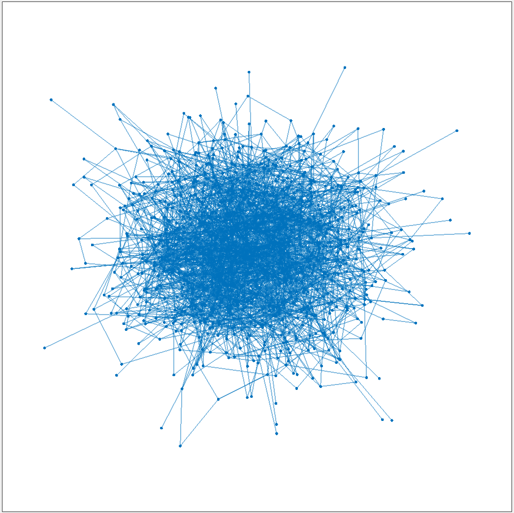
The ADMM and InADMM algorithms are applied to find the shortest path in a random graph as depicted in Figure 3(a). The random graph has $1000$ vertices. The edges are assigned randomly between two vertices with probability $2.6821\times 10^{-5}$ . This yields $2688$ edges. The weight is sampled from uniform distribution on the interval $[10,20]$ . The source and target vertices are randomly picked. The result for the length of the shortest path $\|\beta^{k}\|_{1}$ as a function of iterations, using the ADMM and the InADMM algorithms, is depicted in Figure. 3(b) and 3(c). The dashed line in the Figure represents the exact shortest path length obtained by Dijkstra’s algorithm. It is observed that the lasso solution converges to the exact solution in around $50$ iterations. The running time of each iteration in InADMM in smaller than ADMM, thus the totally running time of InADMM is also smaller than InADMM (empirically $0.6$ of ADMM algorithm).

VI-B Intelligent Scissors

We consider an image processing application of the shortest path problem. The application is intelligent scissors (Live-wire), which is a popular tool for image segmentation [4]. In this application, the pixels of the image form the vertices of a graph, where each pixel is connected via an edge to its $8$ neighbor pixels. With a suitable choice of weights on the edges, the shortest path between two pixels is the boundary of an object [4, Section 3].

We apply the intelligent scissors to the Pikachu image shown in 4(a). The gray-scale of the image and the structure of the edge weights between the pixels are depicted in Figure 4(b) and 4(c) respectively. The picture contains $3420$ pixels (vertices) which yield $13331$ edges. The objective is to distinguish a clear boundary between the Pikachu icon and background. The objective is formulated as finding the shortest path from pixel $(16,6)$ to pixel $(56,30)$ (top left corner to the bottom of Pikachu) as shown in Figure 4(a).

The ADMM algorithm is simulated for this task with the same parameters as before. The resulting shortest path and the convergence of the length of the path are shown in 4(e) and 5(a) respectively. For comparison, the exact shortest path obtained by the Dijkstra’s algorithm is depicted in Figure 4(d). It is observed that the ADMM algorithm provides an approximate path very similar to the exact path in around $300$ iterations.

As for the InADMM algorithm, the tolerance in the CG method is set to $10^{-7}$ . The resulting shortest path and the convergence of the length of the path are shown in 4(f) and 5(b) respectively

VII Conclusion

In this paper, we studied the Lasso formulation of the shortest path problem. We showed that the lasso path solution is equivalent to the shortest path trees that appear in the Dijkstra’s algorithm. And we proposed to apply the ADMM algorithm to estimate the shortest path length for large graphs. Careful analysis of the computational complexity and the distributed implementation of the ADMM, for this particular objective, is subject of future work.

-A Derivation of (16)

For simplicity, we drop the iteration subscript $k$ in our derivations. $D_{\mathcal{A}}$ is the incidence matrix formed by the edges in the active set. The graph formed by $\mathcal{A}$ consist of two disjoint trees $T^{(s)}$ , $T^{(t)}$ , and set of isolated vertices $\Omega$ . We decompose the rows of matrix $D_{\mathcal{A}}$ into rows corresponding to these three subsets, and express $D_{\mathcal{A}}$ according to

\displaystyle D_{\mathcal{A}}=\begin{bmatrix}D_{\mathcal{A}^{(s)}}&{0}\\ 0&0\\ 0&D_{\mathcal{A}^{(t)}}\end{bmatrix}

where $D_{\mathcal{A}^{(s)}}$ and $D_{\mathcal{A}^{(t)}}$ are the incidence matrix for the tree $T^{(s)}$ and $T^{(t)}$ respectively, and $0$ represents the zero matrix of appropriate dimensions. Then,

\displaystyle D_{\mathcal{A}}^{+}=\begin{bmatrix}D_{\mathcal{A}^{(s)}}^{+}&0&0\\ 0&0&D_{\mathcal{A}^{(t)}}^{+}\end{bmatrix}

We use this expression and Lemma II.1 to compute $a$ and $b$ . By definition (11)

	$\displaystyle a$	$\displaystyle=(Q_{\mathcal{A}}^{T}Q_{\mathcal{A}})^{+}Q_{\mathcal{A}}^{T}y=Q_{A}^{+}y=W_{\mathcal{A}}D_{\mathcal{A}}^{+}y$
		$\displaystyle=\begin{bmatrix}-\frac{1}{\|T^{(s)}\|}W_{\mathcal{A}^{(s)}}P^{(s)}\mathbbm{1}_{s}\\ \frac{1}{\|T^{(t)}\|}W_{\mathcal{A}^{(t)}}P^{(t)}\mathbbm{1}_{t}\end{bmatrix}$

where $P^{(s)}$ and $P^{(t)}$ are the path matrix for tree $T^{(s)}$ and $T^{(t)}$ respectively, and $\mathbbm{1}_{t}$ and $\mathbbm{1}_{s}$ are all one vectors of size $|T^{(s)}|$ and $|T^{(t)}|$ respectively. For $b$ ,

	$\displaystyle b$	$\displaystyle=(Q_{\mathcal{A}}^{T}Q_{\mathcal{A}})^{+}s=W_{\mathcal{A}}D_{\mathcal{A}}^{+}(D_{\mathcal{A}}^{T})^{+}W_{\mathcal{A}}s$
		$\displaystyle=\begin{bmatrix}-W_{\mathcal{A}^{(s)}}\Big(P^{(s)}\mathcal{L}^{(s)}-\frac{1}{\|T^{(s)}\|}P^{(s)}\mathbbm{1}_{s}\mathbbm{1}_{s}^{T}\mathcal{L}^{(s)}\Big)\\ W_{\mathcal{A}^{(t)}}\Big(P^{(t)}\mathcal{L}^{(t)}-\frac{1}{\|T^{(t)}\|}P^{(t)}\mathbbm{1}_{t}\mathbbm{1}_{t}^{T}\mathcal{L}^{(t)}\Big)\end{bmatrix}$

where $\mathcal{L}^{(s)}\triangleq-(P^{(s)})^{T}\mathcal{W}_{\mathcal{A}^{(s)}}s$ is a vector of size $|T^{(s)}|$ corresponding to vertices in the tree $T^{(s)}$ . The component of $\mathcal{L}^{(s)}$ , corresponding to vertex $v\in T^{(s)}$ , is equal to $l_{v}^{(s)}$ , i.e. the length of the path from $v$ to the root $s$ . The vector $\mathcal{L}^{(t)}\triangleq(P^{(t)})^{T}\mathcal{W}_{\mathcal{A}^{(t)}}s$ has similar interpretation, but for vertices of tree $T^{(t)}$ .

Putting the results for $a$ and $b$ together, the ratio $a_{j}/b_{j}$ for $e_{j}\in\mathcal{A}^{(s)}$ is

\displaystyle\frac{a_{j}}{b_{j}}

\displaystyle=\frac{\frac{1}{|T^{(s)}|}w_{j}|R_{j}|}{w_{j}(\sum_{v\in R_{j}}l_{v}^{(s)}-\frac{|R_{j}|}{|T^{(s)}|}\sum_{v\in T^{(s)}}l_{v}^{(s)})}

where $R_{j}$ is the set of non-zero components of the $j$ -th row of $P^{(s)}$ . This concludes (16) for $e_{j}\in\mathcal{A}^{(s)}$ . The derivation for $e_{j}\in\mathcal{A}^{(t)}$ is similar.

-B Derivation of (15)

By definition of joining time (12)

\displaystyle t^{\text{join}}_{j}=\frac{\frac{1}{w_{j}}D_{j}^{T}(Q_{\mathcal{A}}a-y)}{\frac{1}{w_{j}}D_{j}^{T}(Q_{\mathcal{A}}b)\pm 1}

(22)

Next, we obtain expressions for the terms in parentheses. For the term in the numerator

	$\displaystyle Q_{\mathcal{A}}a-y$	$\displaystyle=D_{\mathcal{A}}D_{\mathcal{A}}^{+}y-y$
		$\displaystyle=\begin{bmatrix}D_{\mathcal{A}^{(s)}}&{0}\\ 0&0\\ 0&D_{\mathcal{A}^{(t)}}\end{bmatrix}\begin{bmatrix}D_{\mathcal{A}^{(s)}}^{+}&{0}&0\\ 0&0&D_{\mathcal{A}^{(t)}}^{+}\end{bmatrix}y-y$
		$\displaystyle=\begin{bmatrix}-\frac{1}{\|T^{(s)}\|}\mathbbm{1}_{s}\\ 0\\ +\frac{1}{\|T^{(t)}\|}\mathbbm{1}_{t}\end{bmatrix}$

where we used $DD^{+}=I-\frac{1}{\mathbbm{1}^{T}\mathbbm{1}}\mathbbm{1}\mathbbm{1}^{T}$ for each incidence matrix $D=D_{\mathcal{A}^{(s)}}$ and $D=D_{\mathcal{A}^{(t)}}$ . And for the term in the denominator

	$\displaystyle Q_{\mathcal{A}}b$	$\displaystyle=D_{\mathcal{A}}D_{\mathcal{A}}^{+}(D_{\mathcal{A}}^{T})^{+}W_{\mathcal{A}}s=(D_{\mathcal{A}}^{+})^{T}W_{\mathcal{A}}s$
		$\displaystyle=\begin{bmatrix}-\mathcal{L}^{(s)}+\frac{1}{\|T^{(s)}\|}\mathbbm{1}_{s}\mathbbm{1}_{s}^{T}\mathcal{L}^{(s)}\\ 0\\ \mathcal{L}^{(t)}-\frac{1}{\|T^{(t)}\|}\mathbbm{1}_{t}\mathbbm{1}_{t}^{T}\mathcal{L}^{(t)}\end{bmatrix}$

Using these results in (22) and evaluating the expression for $e_{j}$ for each case in (15) concludes (15).

-C Proof of lemma 3.2

The proof is based on [17, lemma 2]. The active set $\mathcal{A}$ is always unique. In Section V, we showed that the active set form two disjoint trees. Hence, $Q_{\mathcal{A}}=\begin{bmatrix}Q_{\mathcal{A}^{(s)}}&Q_{\mathcal{A}^{(t)}}\end{bmatrix}$ where $Q_{\mathcal{A}^{(s)}}=D_{\mathcal{A}^{(s)}}W_{\mathcal{A}^{(s)}}^{-1}$ and $Q_{\mathcal{A}^{(t)}}=D_{\mathcal{A}^{(t)}}W_{\mathcal{A}^{(t)}}^{-1}$ . $D_{\mathcal{A}_{k}^{(s),(t)}}$ are incidence matrices of two trees and $W_{\mathcal{A}_{k}^{(s).(t)}}$ are two diagonal matrices with positive elements. The kernel of incidence matrix of a tree is empty because there is no cycle. Hence, the rank is equal to the number of columns. As a result, the rank of $Q_{\mathcal{A}}$ is equal to $|\mathcal{A}|$ . Then, according to [17, lemma 2] the Lasso solution is unique.

Acknowledgments

Partial funding was provided by NSF under grants 1807664, 1839441, AFOSR under grant FA9550-20-1-0029.

References

[1] C. Wiener, “Ueber eine aufgabe aus der geometria situs,” Mathematische Annalen, vol. 6, no. 1, pp. 29–30, 1873.
[2] G. Tarry, “Le probleme des labyrinthes,” Nouvelles annales de mathématiques: journal des candidats aux écoles polytechnique et normale, vol. 14, pp. 187–190, 1895.
[3] B. M. Waxman, “Routing of multipoint connections,” IEEE journal on selected areas in communications, vol. 6, no. 9, pp. 1617–1622, 1988.
[4] E. N. Mortensen and W. A. Barrett, “Intelligent scissors for image composition,” in Proceedings of the 22nd annual conference on Computer graphics and interactive techniques, 1995, pp. 191–198.
[5] E. W. Dijkstra, “A note on two problems in connexion with graphs,” Numerische mathematik, vol. 1, no. 1, pp. 269–271, 1959.
[6] H. Bast, D. Delling, A. Goldberg, M. Müller-Hannemann, T. Pajor, P. Sanders, D. Wagner, and R. F. Werneck, “Route planning in transportation networks,” in Algorithm engineering. Springer, 2016, pp. 19–80.
[7] R. K. Ahuja, K. Mehlhorn, J. Orlin, and R. E. Tarjan, “Faster algorithms for the shortest path problem,” Journal of the ACM (JACM), vol. 37, no. 2, pp. 213–223, 1990.
[8] P. van Emde Boas, R. Kaas, and E. Zijlstra, “Design and implementation of an efficient priority queue,” Mathematical systems theory, vol. 10, no. 1, pp. 99–127, 1976.
[9] M. L. Fredman and R. E. Tarjan, “Fibonacci heaps and their uses in improved network optimization algorithms,” Journal of the ACM (JACM), vol. 34, no. 3, pp. 596–615, 1987.
[10] M. Potamias, F. Bonchi, C. Castillo, and A. Gionis, “Fast shortest path distance estimation in large networks,” in Proceedings of the 18th ACM conference on Information and knowledge management, 2009, pp. 867–876.
[11] S. Boyd and L. Vandenberghe, Convex optimization. Cambridge university press, 2004.
[12] S. Boyd, N. Parikh, E. Chu, B. Peleato, J. Eckstein et al., “Distributed optimization and statistical learning via the alternating direction method of multipliers,” Foundations and Trends® in Machine learning, vol. 3, no. 1, pp. 1–122, 2011.
[13] R. Tibshirani, “Regression shrinkage and selection via the lasso,” Journal of the Royal Statistical Society: Series B (Methodological), vol. 58, no. 1, pp. 267–288, 1996.
[14] R. B. Bapat, Graphs and matrices. Springer, 2010, vol. 27.
[15] M. Mesbahi and M. Egerstedt, Graph theoretic methods in multiagent networks. Princeton University Press, 2010.
[16] R. K. Ahuja, T. L. Magnanti, and J. B. Orlin, Network flows. Theory, Algorithms, and Applications. Prentice Hall, 1988.
[17] R. J. Tibshirani et al., “The lasso problem and uniqueness,” Electronic Journal of statistics, vol. 7, pp. 1456–1490, 2013.
[18] B. Efron, T. Hastie, I. Johnstone, R. Tibshirani et al., “Least angle regression,” The Annals of statistics, vol. 32, no. 2, pp. 407–499, 2004.
[19] I. Pohl, “Bidirectional and heuristic search in path problems,” Technical Report SLAC-104, Stanford Linear Accelerator Center, Stanford, California, Tech. Rep., 1969.
[20] H. Yue, Q. Yang, X. Wang, and X. Yuan, “Implementing the alternating direction method of multipliers for big datasets: A case study of least absolute shrinkage and selection operator,” SIAM Journal on Scientific Computing, vol. 40, no. 5, pp. A3121–A3156, 2018.
[21] M. R. Hestenes, E. Stiefel et al., “Methods of conjugate gradients for solving linear systems,” Journal of research of the National Bureau of Standards, vol. 49, no. 6, pp. 409–436, 1952.
[22] S. Boyd, N. Parikh, E. Chu, B. Peleato, J. Eckstein et al. (2011) Matlab scripts for alternating direction method of multipliers. [Online]. Available: https://web.stanford.edu/~boyd/papers/admm/lasso/lasso.html