Inference on the History of a Randomly Growing Tree
Abstract
The spread of infectious disease in a human community or the proliferation of fake news on social media can be modeled as a randomly growing tree-shaped graph. The history of the random growth process is often unobserved but contains important information such as the source of the infection. We consider the problem of statistical inference on aspects of the latent history using only a single snapshot of the final tree. Our approach is to apply random labels to the observed unlabeled tree and analyze the resulting distribution of the growth process, conditional on the final outcome. We show that this conditional distribution is tractable under a shape-exchangeability condition, which we introduce here, and that this condition is satisfied for many popular models for randomly growing trees such as uniform attachment, linear preferential attachment and uniform attachment on a -regular tree. For inference of the root under shape-exchangeability, we propose time algorithms for constructing confidence sets with valid frequentist coverage as well as bounds on the expected size of the confidence sets. We also provide efficient sampling algorithms which extend our methods to a wide class of inference problems.
1 Introduction
Many growth processes, such as the transmission of disease in a human population, the proliferation of fake news on social media, the spread of computer viruses on computer networks, and the development of social structures among individuals, can be modeled as a growing tree-shaped network. We visualize the process as a growing tree, as in Figure 1(a), with each individual corresponding to a node labeled by its arrival time and associations between individuals represented by an edge between the corresponding nodes. In the examples mentioned above, the edges of the tree may correspond, respectively, to the transmission of a disease, spread of a rumor, passage of a computer virus, or establishment of a friendship between the connected nodes. For concreteness, we frame the following discussion in the context of disease spread, so that the edges of the tree represent a person-to-person spread of an infection.
In this setting, we assume there is an initial infected individual, called the root, at time . At each discrete time step , a new individual becomes infected by one of the individuals previously infected at times according to a probability distribution that depends on the past history of the process. By tracking the infection through the growth of the corresponding infection tree (as in Figure 1(a)), the process of infection thus produces a sequence of trees which represents the complete history of infection in the population. In particular, is a tree with nodes and a directed edge indicating that node passed the infection to node . Equivalently, labels can be assigned to the nodes of according to the time at which each node arrives, so that any edge is immediately interpreted as a transmission from the node with the lower label to the one with the higher label.
(a) 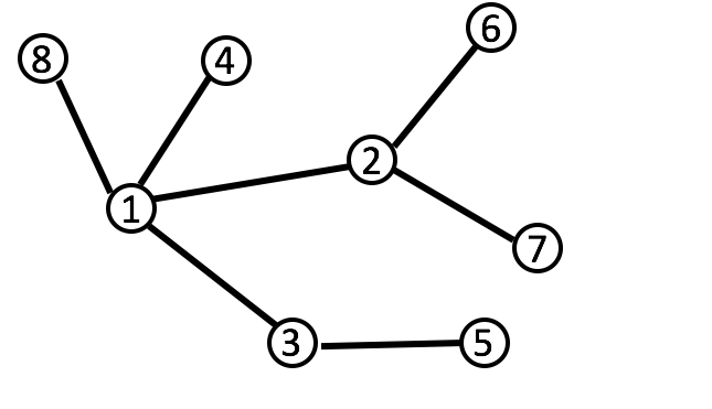 (b)
(b) 
In epidemiological applications, the infection history is important for enacting measures which prevent further spread, such as quarantining and testing. But in many cases the complete infection history is not fully observable. In the 2020 outbreak of Covid-19, for example, long incubation periods and asymptomatic spreading leads to incompleteness in the observed infection history (i.e., some or many edges in the infection tree are unobserved) as well as uncertainty about the direction of spread for those edges which are observed, as shown in Figure 1(b). Here we consider the problem of inferring properties of the disease history based on such partial observations of the infection spread. Properties of special importance include inference of the root node (so-called ‘patient-zero’) and inference of infection time. We develop our methods in the specific context in which the contact pattern has been observed (i.e., the ‘shape’ of the infection tree is known but its directions are not). We discuss some relaxations to this assumption and limitations of our methods in Section 6.
Suppose that a disease has been transmitted among individuals (as illustrated in Figure 1(a)) but only the contact pattern is observed (as in Figure 1(b)). We propose a methodological framework for answering general inference questions about the infection spread based on the observed contact pattern. In the context of disease spread, important relevant questions include inference of so-called ‘patient-zero’ (i.e., the initial source of infection) and also the time at which specific individuals became infected. Our proposed method efficiently computes the conditional probability of the disease transmission history given the observed contact process. These conditional probabilities enable us to construct valid confidence sets for the inference questions of interest. These inference procedures may be applied in social media networks to help identify key spreaders and promoters of fake news or applied on the infection pattern of an epidemic (often obtained from contact tracing) to localize patient-zero or to reconstruct the chain of infection (Hens et al. 2012; Keeling and Eames 2005).
1.1 Literature review
Researchers in statistics (Kolaczyk 2009), computer science (Bollobás et al. 2001), engineering, and physics (Callaway et al. 2000) have studied the probabilistic properties of various random growth processes of networks, including popular models such as the preferential attachment model (Barabási and Albert 1999). A line of research in the physics and engineering literature explores the problem of full or partial recovery of the network history based on a final snapshot (Young et al. 2019; Cantwell et al. 2019; Timár et al. 2020; Sreedharan et al. 2019; Magner et al. 2018). However, the problem of statistical inference on the history of a network growth process has been studied only recently. In statistics, most existing work focuses on the problem of root estimation (Shah and Zaman 2011; Shah and Zaman 2016; Fioriti et al. 2014; Shelke and Attar 2019) and root inference (Bubeck, Devroye and Lugosi 2017). The latter work by Bubeck, Devroye and Lugosi 2017 shows that one can construct a confidence set of the root whose size does not increase with the size of the network . These directions are further developed by Bubeck, Eldan, Mossel and Rácz 2017, by Lugosi et al. 2019 and Devroye and Reddad 2018, who consider inference on a seed tree, by Shah and Zaman 2016, who analyze situations where consistent root estimation is possible, and by Khim and Loh 2017, who extend the results of Bubeck, Devroye and Lugosi 2017 to the setting of uniform attachment on a -regular tree. More recently, Banerjee and Bhamidi 2020 derives tight bounds on the size of confidence set of the root constructed from Jordan centrality. These results, although theoretically sound, do not give a practical method for inferring the root of a tree based on an observed contact pattern. For example, the confidence set algorithms in Bubeck, Devroye and Lugosi 2017 and Khim and Loh 2017 (described in detail in Section 2.3) only give asymptotic coverage guarantees that hold under specific model assumptions and tend to be too conservative for practical purposes; see the numerical examples in Section 5.1 for further discussion.
1.2 Summary of Approach
In this paper, we address the above issues by proposing a new approach for inference on the history of a randomly growing tree. Our approach is to randomly relabel the nodes of the observed shape to obtain a random tree whose labels are random but whose shape corresponds to that of the observed contact pattern. Random relabeling thus induces a latent sequence of subtrees which represents the history of . We study the conditional distribution of the history and show that the conditional distribution is tractable under a shape-exchangeability property, a distributional invariance property which is satisfied by the most common instances of the preferential attachment models including linear preferential attachment, uniform attachment and -regular uniform attachment.
For most of the paper, we focus on the problem of root inference, where our proposed method has a coverage guarantee for all and produces informative and computationally efficient confidence sets even for trees of millions of nodes. However, our approach is also applicable to a wide class of other inference problems such as arrival time inference and inference of the initial subtree given the final shape.
1.3 Summary of Methodology
Although the problem of inferring the root node is conceptually simple, we need a number of technical definitions in the main paper to address subtle complications that arise from a formal analysis. To aid readers who are interested in a conceptual understanding, we first provide a short informal discussion of our methodology.
For a given tree and a node , we can think of a single realization of how the tree “grew” from node as an ordered sequence of the nodes where . Not all ordered sequences are possible since the tree must be connected at all times and so we define as the subset of allowable permutations of the nodes that starts at node and results in tree (see Figure 3). Interestingly, for a class of preferential attachment tree models including both uniform attachment and linear preferential attachment (Examples 1 and 2), the conditional distribution of the growth realization is uniform over the set of all allowable sequences (Proposition 3 and Theorem 4). Moreover, the cardinality can be computed in linear time (Proposition 5). Therefore, we can compute the conditional root probability , as the fraction of all allowable permutations that starts at node , and construct a Bayesian credible set by taking the nodes with the highest conditional root probabilities. We prove that such a credible set also has valid Frequentist coverage at exactly the same level (Theorem 1).
The paper is organized as follows. In Section 2 we define the problem and review some earlier work. In Section 3 we describe our approach using random labeling and the shape exchangeability condition. In Section 4 we discuss general inference problems for observed contact patterns. In Section 5 we show some simulation studies and illustrate our methods on flu data from a London school.
1.4 Notation:
For , we write and . We let denote a labeled tree where is the finite set of nodes (generally taken to be where is the size of the tree) and is the set of edges.
For two finite sets of the same size, we write as the set of all bijections between and . For two labeled trees , we write for if is an edge in if and only if is an edge in . In this case, we say that is an isomorphism between and . We note that for any labeled tree and any bijection , is always a valid tree that represents the result of relabeling the nodes of by . For a labeled tree and a subset of nodes , we write as the (possibly disconnected) subgraph of restricted only to the nodes in .
Throughout the paper, we use bold upper-case letters such as to denote a random tree and bold lower-case letters such as to denote a fixed tree. For any two random objects , we write if they are equal in distribution.
2 Model and Problem Definition
2.1 Markovian tree growth processes
Following the terminology used in discrete mathematics, we define a labeled tree with nodes as a recursive tree if and if the subtree , obtained by removing all nodes except those with labels , is connected for every . In other words, any path from node to any other node must be increasing in the node labels. Equivalently, we may view a recursive tree as a map with indicating that the parent of is , for , and indicating that node is the root of . Figure 1(a) illustrates a recursive tree with 8 nodes. We write to denote the set of all recursive trees with nodes.
For recursive trees with node labels and , respectively, for , we write if . That is, indicates that is the subtree of obtained by removing all nodes and edges from except those labeled in . For , we call and compatible if . A family such that for all is called mutually compatible.
A Markovian tree growth process is a mutually compatible family of random recursive trees such that for each and
| (1) |
for some family of transition probabilities . Any such process can therefore be constructed by sequentially adding nodes at discrete times according to these transition probabilities and labeling the nodes of by their arrival time.
Example 1.
For a straightforward example of a growth process, define
so that new nodes attach to existing nodes uniformly at each time. The resulting process is called the uniform attachment (UA) model. We note that in discrete probability, UA trees are called ”random recursive trees” because it is uniform over the set of all distinct recursive trees (see e.g. Drmota 2009). We use the term ”random recursive tree” in a more general sense in that we allow a random recursive tree to have any Markovian distribution.
Example 2.
For another popular example, let denote the degree of node in and for let denote the unique node of to which the node labeled connects to form . We start with one node, attach another node to it, and then define transition probabilities by
The resulting tree process is called the linear preferential attachment model (LPA), as nodes with high degree tend to accumulate more connections. In discrete probability, LPA trees are also referred to as random plane-oriented recursive trees (see e.g. Drmota 2009).
Example 3.
To generalize the previous two examples, we define a general class of preferential attachment (PA) processes indexed by a fixed function as follows. For short, we call these processes. Given such a function , we generate as a singleton node with label and, for each , generate as a random tree where we
- 1.
choose an existing node of with probability proportional to , where denotes the degree of node in ,
- 2.
and add edge to tree to form .
The resulting transition probabilities of this process thus satisfy
Common examples of the function include (a) uniform attachment where for all (as in Example 1), (b) linear preferential attachment where (as in Example 2), (c) uniform attachment on a -regular tree where for some , and (d) sublinear preferential attachment where for some . We also note that Gao et al. 2017 studies the estimation of the parameter function .
For labeled trees , not necessarily recursive, we write if there exists a such that . We define the shape of as the equivalence class of all that are equivalent to up to some relabeling,
A shape is typically referred to as an “unlabeled tree” or just a “tree”. We prefer the term “shape” here to emphasize that does not refer to a single tree but rather to an equivalence class of all trees with a given structure. Figure 1(b) shows the ‘shape’ of the labeled tree in Figure 1(a). In our analysis, this ‘shape’ represents the set of all trees that produce the same structure after removing labels.
Since is an equivalence class, we need to first define what it means to refer to the nodes of . To that end, we let be an alphabet of distinct letters and represent the shape by an arbitrary labeled tree with node labels . We may now refer to the nodes of through its alphabetically labeled representation . For convenience, we define as the set of all labeled trees with nodes whose labels take values in the alphabet .
We note that it is necessary to work with a labeled representation of a shape because (i) our inference questions make reference to properties of specific nodes (e.g., a particular node being the root) and (ii) computer programs require as input a labeled tree instead of an equivalent class of labeled trees. Because the choice of the labeled representation is arbitrary, we only consider inference methods that are independent of the choice of the representation. We formalize this with the notion of labeling-equivariance in Remark 2.
2.2 Inference Problem
Let be a Markovian growth process for which we observe only the unlabeled shape for some . For a labeled representation whose node labels take values in , we say that the root of is if the node labeled in the labeled representation corresponds to the root of . More precisely, letting be an unobserved bijection such that , we define
| (2) |
Remark 1.
It is important to note that the root node depends on the choice of the isomorphism ; there could exist such that and that ; see Figure 2. This is because multiple nodes of an unlabeled shape can be indistinguishable (see (15) in Section 3.6 for a formal definition of indistinguishable nodes). We show in Remark 2 that this issue does not pose a problem to our inference procedure as long as we only consider labeling-equivariant confidence sets.

Formally, the problem of root node inference is to construct, for given a confidence level , a confidence set such that
| (3) |
As a trivial solution is to let be the set of all nodes , an important aspect of the inference problem is to make the confidence set as small as possible while still maintaining valid coverage (3). We note that the root node cannot be consistently estimated since, for a tree of 2 nodes, it is impossible to distinguish which one is the root.
Remark 2.
Since our observation is the unlabeled network , it is natural to require the confidence set to be labeling-equivariant so it does not depend on the choice of the labeled representation . More precisely, for any , we require
| (4) |
where is the set containing the image of all members of under . In particular, if is an automorphism in the sense that , we require to be invariant with respect to .
The definition of the root node (2) relies on a particular isomorphism . However, for a labeling-equivariant confidence set, as in (4), the probability of coverage (3) does not depend on this choice of the isomorphism. Indeed, if we write as the root node with respect to , then, for any , the node labeled is the root node under an alternative labeling and we see that if and only if .
An unlabeled shape may contain indistinguishable nodes that are given different labels in a labeled representation. For example, the nodes labeled in the labeled tree in Figure 2 are indistinguishable. However, any set of indistinguishable nodes must be either all included in or all excluded from a labeling-equivariant confidence set by the fact that such confidence sets are invariant with respect to automorphisms.
Although we focus on root inference, the approach that we develop are applicable to more general inference problems such as inferring the arrival time of a particular node. We describe these in detail in Section 4.
2.3 Previous work on root inference
For the problem of root node inference, Bubeck, Devroye and Lugosi 2017 consider procedures that assign a centrality score to each node of the observed shape and then take the largest nodes to be the confidence set where is a size function whose value depends on the underlying distribution. More precisely, let be the observed shape with labeled representation whose node labels take values in . Let be a scoring function and let be an integer for any . Assuming that the nodes are sorted so that , define . The function is labeling-equivariant in that for any , we have . The induced confidence set is therefore also labeling-equivariant.
With these definitions, Bubeck, Devroye and Lugosi 2017 show that if the random recursive tree has the uniform attachment distribution, then there exists a function such that, with any for universal constants , we have
In other words, so long as is large enough, has asymptotic confidence coverage of . If is distributed according to the preferential attachment distribution, then Bubeck, Devroye and Lugosi 2017 show that there exists such that has asymptotic coverage when for some universal constant . Lower bounds on the size are also provided. We also note that after the completion of this manuscript, Banerjee and Bhamidi 2020 further improved the upper bound on to in the linear preferential attachment setting.
If is distributed according to uniform attachment on -regular trees for some , then Khim and Loh 2017 shows that there exists such that has asymptotic coverage when for some constant depending only on .
These above results are surprising in that as the size of the tree increases, the size of the confidence set can remain constant—the intuition for this being that the “center” of the growing tree does not move significantly as new nodes arrive (Jog and Loh 2018; Jog and Loh 2016; Bubeck et al. 2015). However, these results have a number of shortcomings that make them impractical for real applications. First, the confidence guarantee is asymptotic and does not hold in . Second, the bound on the size is theoretical and too conservative to be useful. As we show in Figures 3 and 4, the bound given in each case tends to be excessively conservative even for relatively large values of . Third, it is necessary to know the model of the random recursive tree in order to choose the correct size . In the next section, we present an alternative approach to constructing confidence sets for the root node that addresses all these shortcomings.
The choice of the scoring function is crucial. The ideal choice is the likelihood, which is complicated to express so we defer its formal definition to equation (16) in Section 3.6 to avoid interrupting the flow of exposition. Bubeck, Devroye and Lugosi 2017 remark that the likelihood is computationally intensive and analyzes a relaxation instead. One such relaxation is based on taking products of the sizes of the subtrees (termed by Shah and Zaman 2011 as rumour centrality) and it plays an important role in our approach; see (13) for a precise definition. Interestingly, one implication of our work is that this product-of-subtree-sizes relaxation in fact induces the same ordering of the nodes as the true likelihood so that the confidence set constructed from the relaxation is the same as that from the true likelihood.
3 Approach
In this section, we describe our approach to root inference through the notion of label randomization and shape exchangeability. In Section 4, we show that the same approach applies to various other inference problems as well.
3.1 Random Labeling
Let be a random recursive tree and let be its shape. Given and any alphabetically labeled representation , we may independently generate a random bijection uniformly in and apply it onto to obtain a randomly labeled tree . We note here that the resulting object satisfies where is another uniform random bijection chosen independently of and . In particular, the marginal distribution of does not depend on the choice of representative . To fix notation, from now on we write to denote a random labeled tree generated in this way.

For any , we also define , where we interpret as the domain restriction of the random bijection defined on . In this way, . Since each of the random subtrees has the same shape as , the random shape has the same distribution as . In particular, the label of the singleton is drawn uniformly from and each subsequent node added at time is drawn uniformly from . We illustrate the definitions associated with label randomization in Figure 3.
We can interpret label randomization as an augmentation of the probability space. An outcome for a Markov tree growth process is a recursive tree whereas an outcome for the label randomized sequence is a pair where is a recursive tree and is a bijection from to . By defining , we obtain a bijective correspondence between a pair and a sequence of nested subtrees where . We define any such sequence of nested subtrees (equivalently any pair ) as a tree history, or simply a history for short. Intuitively, is the isomorphism that gives the ordering information of the nodes in as the node labels of take value in the alphabet . Given the correspondence between the sequence and the pair , the probability of a history is given by
| (5) |
To give a concrete example, let the random recursive tree be generated from preferential attachment process . Then, the corresponding sequence of random trees have the distribution where is a singleton node drawn uniformly from and for , we select a node with probability proportional to , select a node uniformly at random, and add the edge to to form .
Suppose we have data in the form of a given unlabeled shape with an arbitrarily alphabetically labeled representation whose node labels take values in . We may apply label randomization if necessary to assume without the loss of generality that is an outcome of the randomly labeled tree . Our inference approach is based on the conditional distribution of a history
| (6) |
For example, for and an observed shape with alphabetically labeled representation , we may interpret as the probability of being the root node conditional on observing the shape .
Label randomization is a data augmentation scheme that simplifies the analysis and the computation. We can define the conditional probability of a node being the root without the use of label randomization (see Remark 5) but we show in Theorem 8 that the alternative definition is equivalent to the conditional root probability with label randomization. The calculation in (5) makes this approach precise.
Our proposed approach to either compute or approximate the conditional distribution of a history given a randomly labeled final state is especially natural for the purpose of developing a statistical framework which applies to a broad class of inference problems about the tree history. This general strategy can also be found in approaches posed independently within other disciplines, as in the similar conditional probability-based approaches in the physics literature (Young et al. 2019; Cantwell et al. 2019; Timár et al. 2020) and the randomized labeling framework proposed for tree reconstruction algorithms in computer science (Sreedharan et al. 2019; Magner et al. 2018).
3.2 Root Inference
With the definition of the conditional history (6), a natural approach for inferring the root is to construct a level credible set by iteratively adding nodes with the largest conditional root probabilities until the sum of the conditional root probabilities among the nodes in the set exceed . More precisely, let our data be an unlabeled shape with an alphabetically labeled representation , that is, has node labels in . We sort the nodes of such that
| (7) |
and we define
| (8) |
We then define the -credible set as
| (9) |
If there are no ties in the conditional root probabilities (7), then is the smallest subset of such that
| (10) |
When there are ties however, the second condition in our definition of dictates that we resolve ties by including all nodes with equal conditional root probabilities. Breaking ties by inclusion ensures that is labeling-equivariant.
In general, credible sets do not have valid Frequentist confidence coverage. However, our next theorem shows that in our setting, the credible set is in fact an honest confidence set.
Theorem 1.
Let be a random recursive tree and let be any arbitrary labeled representation (with labels taking values in ) of the observed shape , and let be any isomorphism such that . We have that, for any ,
Proof.
We first claim that, for a given shape with an alphabetically labeled representation , the credible set is labeling-equivariant (cf. Remark 2) in the sense that for any , we have that .
Indeed, since , we have that, for any ,
Therefore, for any , we have that if and only if . Since is constructed by taking the top elements of that maximizes the cumulative conditional root probabilities, the claim follows.
Now, let be such that and let be a random bijection drawn uniformly in . Then,
where the penultimate equality follows from the labeling-equivariance of and where the last inequality follows because for any labeled tree (with labels in ) by the definition of . ∎
Theorem 1 shows that we may obtain a valid confidence set by constructing a credible set. The credible set can be efficiently computed for a class of tree growth processes that we describe in the next section.
3.3 Shape exchangeable growth process
The conditional history distribution (6) can be intractable for a general Markov tree growth process but it has an elegant characterization when the growth process satisfies a shape exchangeability condition.
Definition 2.
A random recursive tree process is shape exchangeable if for all
| (11) |
Remark 3.
Our definition of shape exchangeable trees follows recent developments in the theory of exchangeability, in particular the theory of relative exchangeability (Crane and Towsner 2018), in which the distribution is invariant with respect to a subgroup of permutations that respect an underlying structure. In the case of shape exchangeability, the shape determines an isomorphism class of tree histories, and shape exchangeability implies that every member of a given isomorphism class is equiprobable. Note, in particular, that the exchangeability condition applies to the distribution on recursive trees (i.e., tree histories), in the sense that two histories with the same shape have the same probability. Shape exchangeability does not imply that each shape has the same probability of occurring.
Immediate examples of shape exchangeable processes include the uniform attachment and the linear preferential attachment models from Examples 1 and 2. Theorem 4 shows that these two classes combine to characterize the class of all shape exchangeable processes.
In general, if a random recursive tree is shape exchangeable, then the conditional probability (6) of the random sequence of label-randomized trees takes on a simple form as shown in Proposition 3 below. We define some necessary concepts and notation before stating the result.
Let be a labeled tree with nodes labeled by . We define as set of all histories that result in . We may associate each distinct history with a sequence such that for every . We thus have that
that is, is a set of the permutations of the node label set that satisfy the constraint that restricted to is a connected sub-tree for any . Equivalently, we may define as the set of all label bijections such that is a recursive tree.
We write the denote the number of distinct histories of . It is clear that depends only on the shape . Moreover, for a particular node , we define as the set of all histories rooted at the node , that is,
Proposition 3.
Suppose is shape exchangeable and let be the randomly labeled history. Then, for any history with labels in , we have that
Proof.
Suppose is shape exchangeable. Let be any labeled tree with nodes labels in let and be two histories of . By (5) and shape exchangeability of , we have that
Therefore,
for all histories and corresponding to . It follows that the conditional probability is equal for all histories, and thus the conditional distribution of the history given the final state is uniform over , as was to be proven. ∎
Theorem 4.
Let and let be a process. is shape exchangeable if and only if has the form
| (12) |
for satisfying either
- •
and for some integer or
- •
and .
Remark 4.
Theorem 4 shows that shape exchangeability encompasses three widely studied tree growth processes. Both the linear preferential attachment process, where , and the uniform attachment, where , are shape exchangeable. In addition, we note that the case where is negative corresponds to uniform attachment on the -regular tree, i.e., for some . However, the sublinear preferential attachment process where for some is not shape exchangeable; we discuss inference procedures for non-shape exchangeable trees in Section 4.2.
Thus, for uniform attachment, linear preferential attachment, and -regular uniform attachment processes, Proposition 3 and Theorem 4 combine to imply that inference about measurable functions of the unobserved history can be performed without knowing the and parameters governing the process. In particular, valid confidence sets can be constructed by observing only the shape of the final state.
Equivalently, if has the distribution where , then, by Proposition 3, the shape is a sufficient statistic for and and knowledge of the history is ancillary to the estimation of and . We note that Gao et al. 2017 makes a similar informal statement regarding the estimation of the parameter function .
3.4 Computing conditional root probabilities
Shape exchangeable tree processes are naturally suited to the inference questions highlighted in Section 2.2. For example, for the question of root inference, suppose we observe with an arbitrary labeled representation , then we may compute, for each node of ,
| (13) |
In fact, the numerator coincides with the notion of rumor centrality defined by Shah and Zaman 2011 for the purpose of estimating the root node. The following proposition summarizes a characterization of given in Section IIIA of Shah and Zaman 2011. We note that Knuth 1997 made the same observation in the context of counting the number of ways to linearize a partial ordering.
Proposition 5.
(Knuth 1997; Shah and Zaman 2011)
Let be a labeled tree with and let . Viewing as being rooted at , define, for every node , the tree as the sub-tree of rooted at and as the size of . Writing as the neighbors of , we have that
Using the fact that for any node and its parent node , viewing as being rooted at , Shah and Zaman 2011 derive an algorithm for counting the number of histories for all possible roots . We give the details in Algorithm 1 for reader’s convenience. Using Algorithm 1, we conclude that the overall runtime of computing the confidence set is since we need to also peform a sort.
Input: a labeled tree .
Output: for all nodes .
3.5 Size of the confidence set
In this section, we use the results of Bubeck, Devroye and Lugosi 2017 and Khim and Loh 2017 to provide a theoretical analysis of the size of the confidence set . We also provide empirical studies of the size in our simulation studies in Section 5.1.
In Section 3.2, we defined for a fixed labeled tree in (8) which is the size of our confidence set . In this section, we analyze a slight variation where, assuming that the nodes are sorted in decreasing order by their conditional root probabilities, we define
| (14) |
where is defined formally in (15) and is intuitively the set of nodes equivalent to in the tree . If we construct , then, for any fixed labeled tree , the set is the smallest labeling-equivariant subset of such that . In other words, is the optimal credible set for any fixed Bayesian coverage level. We may directly apply the argument in the proof of Theorem 1 to show that , defined with respect to (14) is also a valid Frequentist confidence set at the same level . We note that, for practical applications, we prefer (8) over (14); we observe in simulations that the two are almost always equivalent. The next lemma compares the size of with the optimal Frequentist confidence set.
Lemma 6.
Let be arbitrary, let be a random recursive tree, and let be an alphabetically labeled representation of . Let be defined as in (14). Fix any and let be any confidence set for the root node that is labeling-equivariant and has asymptotic coverage level , that is, for any labeling that satisfies . Then, we have that
By letting for example, Lemma 6 shows that, with probability at least , the size of our confidence set is no larger than the optimal asymptotically valid confidence set at a higher level . We defer the proof of Lemma 6 to Section S2 in the appendix.
We now define , , and, for an integer , where are universal constants and where is a constant that depend only on . We may then use Lemma 6 in conjunction with results from Bubeck, Devroye and Lugosi 2017 and Khim and Loh 2017 to bound the size of our confidence sets.
Corollary 7.
Let be arbitrary, let be a random recursive tree, and let be an arbitrary labeled representation of whose node labels take values in . Let be defined as in (14).
If is distributed according to the uniform attachment model, we have that, for all ,
If is distributed according to linear preferential attachment,
If, for some integer , is distributed according to uniform attachment on a -regular tree, then
Proof.
By Bubeck, Devroye and Lugosi 2017, we know that when has the uniform attachment distribution, there exists a labeling-equivariant scoring function such that for any , the set with size contains the root with at least probability asymptotically. The first part of the Theorem thus follows.
We may obtain the other two claims of the Theorem in identical ways by using Bubeck, Devroye and Lugosi 2017 and Khim and Loh 2017. ∎
From Corollary 7, we see that in all three cases, the random size is as , which shows that the size of the confidence set is of a constant order even when the number of nodes tends to infinity. Moreover, the median size is asymptotically at most respectively for each of the three cases. As we show in our simulation studies (see e.g. Tables 2), these bounds tend to be very conservative.
Since the size of our confidence set depends on the observed tree , it is adaptive to the underlying distribution of . In contrast, the sizes of the confidence sets considered in Bubeck, Devroye and Lugosi 2017 and Khim and Loh 2017 depend only on and hence must be chosen with knowledge of the true model.
3.6 Equivalence to maximum likelihood
In this section, we show that is proportional to the likelihood of being the root on observing . Thus, any confidence sets created by ordering the nodes according to their conditional root probability also maximizes the likelihood. We first follow Bubeck, Devroye and Lugosi 2017 to derive the likelihood of a node being the root on observing the unlabeled shape .
Given any labeled trees , not necessarily recursive, and two nodes , we say that and have equivalent rooted shape (written ) if there exists an isomorphism such that and . We then define the rooted shape of as the equivalence class
We give examples of rooted shapes with 4 nodes in Figure 4.
For any labeled tree , not necessarily recursive, and for any node , we define the set of indistinguishable nodes as
| (15) |
as the set of all nodes where rooting at either node or yield the same rooted shape. In other words, is the set of all the nodes of that are indistinguishable from once we remove the node labels. We give examples of indistinguishable nodes in Figure 4.
Let be a random recursive tree and suppose we observe that where is a shape with an arbitrary alphabetically labeled representation . For any node , the likelihood that any node in is the root is then the sum of the probabilities of all outcomes of the random recursive tree that has the same rooted shape as . Since may contain multiple nodes, we then divide by the size of the set to obtain the likelihood of node being the root.
To be precise, for a labeled tree and a node , we define
which is the set of all distinct recursive trees that have the same rooted shape as rooted at . The likelihood of a node is then
| (16) |
where we divide by to account for multiplicity of indistinguishable nodes. If is shape exchangeable, then is a constant for any recursive tree with the same shape as that of and thus
The number of distinct recursive trees is in general smaller than the number of distinct histories , see for example Figure 4. Bubeck, Devroye and Lugosi 2017 derives an exact expression of the in terms of isomorphism classes of the subtrees of . This is difficult to compute however as it requires counting the automorphism classes of the subtrees.

Since the likelihood is based on counting the recursive trees and the conditional root probability is based on the counting the histories , it is not obvious how to relate the two. Our main result this section is the next proposition which shows that they in fact induce the same ordering of the nodes of a tree . We note this proposition strengthens the existing results in literature; in particular, it implies that Bubeck, Devroye and Lugosi 2017 applies in fact to the exact MLE instead of an approximate MLE as previously believed.
Theorem 8.
Let be a random recursive tree, not necessarily shape exchangeable, and let be the corresponding random history. For any labeled tree with node labels taking value in , we have that, for all ,
Remark 5.
From Theorem 8, we see that, for a labeled tree and a node , we can define the conditional probability that is the root node with the quantity , without the use of the label randomized tree . We divide by to address the issue that there may be multiple nodes that are indistinguishable from node . Theorem 8 shows that this is equivalent to the the label randomized conditional probability . We use the latter expression for its simplicity.
4 General Inference Problems
The approach that we take for root inference and the structural properties that we proved for shape exchangeable processes may also be used for general questions of interest about unobserved histories. To formalize general inference problems, we let be the labeled representation of the observed shape and let be the label bijection that gives . Let be a discrete set and let be a function. For a confidence level , our inference problem is to construct a confidence set such that
| (17) |
Example 4.
By taking and , we obtain the root inference problem (Section 2.2). A natural extension of the root inference problem is to infer the earliest nodes to appear, which is known as the seed-tree inference and has been studied by Devroye and Reddad 2018; in seed-tree inference, for a given , we let be the set of all subtrees of of size and let .
Example 5.
For a fixed node , we may infer the time at which it appeared in the observed tree. We let and define the random arrival time of node as
The problem is then to construct, for a given , a confidence set such that the true arrival time is contained in with probability at least . This problem is well-defined for confidence sets that satisfy a labeling-equivariance condition; we defer the technical details to Section S4 of the appendix.
We may consider a number of other inference problems, e.g., given a subset of nodes , what is the order in which they were infected? The approach given below can be applied quite generally to most conceivable questions of this kind. These may all be formalized in a manner identical to the examples that we have shown.
In these cases, we replace an exact calculation of the conditional probability by Monte Carlo approximation. In particular, we derive two different computationally efficient sampling protocols to generate a history of a given tree uniformly at random. To make the discussion concrete, consider again the arrival time of a given node : for such that . In this case, for a given tree , we may construct the confidence set by first computing as the smallest subset of such that
where is a random bijection distributed uniformly in such that and where we take as the empty set. Following Theorem 1, we may again show that has valid Frequentist coverage; we defer the formal statement and proof of this claim to Section S4.
To compute the confidence set , we need to compute, for each , the conditional probability
| (18) |
We propose a Monte Carlo approximation where we generate independent samples from the conditional history distribution . For an event , we may then approximate
For example, we may approximate the probability of node arriving at time (see (18)) by
In the next section, we assume shape exchangeability and show two exact sampling schemes which allow us to efficiently carry out this approach. In Section 4.2, we devise an importance sampling scheme for computing the conditional probability under a general process, not necessarily shape exchangeable.
4.1 Sampling for shape exchangeable processes
If is shape exchangeable, then we may generate a sample by drawing a single history from the set uniformly at random. In general, the total number of histories is large, but uniform sampling can be carried out sequentially by either
- (i)
forward sampling, which builds up a realization from the conditional distribution by a sequential process of adding nodes to the following scheme, or
- (ii)
backward sampling, which recreates a history from the observed shape by sequentially removing nodes according to the correct conditional distributions.
Throughout this section, it will be convenient to think of a history as an ordered sequence where for every .
4.1.1 Forward sampling
Conditional on the final shape , a uniform random history can be generated by an analog to the Pólya urn process. We generate the first element (root) of the history from the distribution over , where the conditional root probability distribution can be computed in time through Algorithm 1. Once the root of the history is fixed, we then sequentially choose the next node by size-biased sampling based on the size of the subtree rooted root at away from the root .
More explicitly, let be a tree labeled in and rooted at . For any , we write to denote the subtree of rooted at node away from and as the size of the subtree. Given the shape of , we generate a history by
- •
sampling from and
- •
given , sampling from among the remaining nodes in according to
We note that (• ‣ 4.1.1) is a well-defined probability distribution because once we have fixed the first nodes of the history , the probability on the left hand side of (• ‣ 4.1.1) is positive only for a neighbor of . Summing over all neighbors of gives exactly the denominator of (• ‣ 4.1.1).
The coming proposition shows that the result of this process is a valid draw from the conditional distribution of the history given .
Proposition 9.
Let be a shape exchangeable preferential attachment process and be a randomly labeled element of . For any sequence of nodes , the conditional distribution of given the conditional distribution in (• ‣ 4.1.1).
Proof.
Let the labeled tree be fixed and suppose is a random history where for all and where the probabilities of are specified by (• ‣ 4.1.1).
Proposition 9 states that to generate the second node of the history given that the first node is , we consider all neighbors of (where denotes the number of neighbors of ) and choose with probability proportional to the size of the subtree . Continuing in this way, once we have generated the first nodes of the history, we consider all neighbors of the subtree and again choose a neighbor with probability proportional to the size of the subtree .
The existence of such a sampling scheme for shape exchangeable processes is closely related to other sequential constructions for generating samples from exchangeable processes, such as the Chinese restaurant process found throughout the Bayesian nonparametrics and combinatorial probability literature; see, e.g., Crane 2016 for an overview of various constructions for exchangeable partition processes. The size-biased sampling without replacement in the above can also be related to general Polya urn schemes which are known to produce exchangeable sequences.
The computational complexity required to compute the size of all the subtrees is linear in total number of nodes because we can use a bottom-up procedure that makes a single pass through all of the nodes of the tree. Therefore, the computational complexity of generating the first elements of the history depends on the number of neighbors . The number of neighbors could be of order and thus requiring time to generate a full history .
We can improve the runtime of generating a full history to in the worst case in Algorithm 2. The algorithm proceeds by drawing the first node of the history from distribution (13); we now view the input labeled tree as being rooted at . We then generate a random permutation of the node labels and modify the random permutation by swapping the position of a node with that of its parent if appears in the permutation before . We continue until the random permutation satisfies the constraints necessary to be a valid history. The modification process can be done efficiently through sorting so that the overall runtime is at most where is the length of the longest path (diameter) of the tree , as shown in the following proposition. We note that for uniform attachment or linear preferential attachment trees, the diameter is (see e.g. Drmota 2009 and Bhamidi 2007) and so the runtime of Algorithm 2 is typically .
Input: Labeled tree whose node labels take value in .
Output: A history represented as a sequence where .
Proposition 10.
Proof.
It is clear that the output is a valid history. Suppose for some , then for some neighbor of if and only if for some node in the subtree rooted at . Since is a random permutation, the event that for some is exactly .
Now assume that we have generated the first elements of the history . Again, the event that for some neighboring node of if and only if for some , which occurs with probability exactly . By Proposition 9, it thus holds that is uniform sample from
To prove the runtime of Algorithm 2, we note that may be generated in time, for example by the Knuth-Fisher-Yates shuffle algorithm (Fisher and Yates 1943). For each node , we let denote the number of ancestor nodes, including itself, not in the set when the algorithm is at iteration . It then holds that since each node is placed in the set as soon as it is visited by the algorithm. Thus,
which proves the proposition. ∎
4.1.2 Backward sampling
We may also generate a history , equivalently represented as a sequence of nodes , from the conditional distribution by iterative removing one leaf a time.
If is shape exchangeable, then we have by Proposition 3 that for any labeled tree and any leaf node that
| (21) |
Thus, given an observed shape and with an alphabetically labeled representation , we may reconstruct a history leading to that shape by recursively removing leaves according to (21). Naive implementation of backward sampling has a runtime of but, by observing that
one may first draw a random node from the distribution and then remove a random leaf node drawn with probability . The quantities for all leaf node can be computed jointly in time by precomputing the size of the subtrees. The overall runtime of backward sampling is therefore , which is typically for uniform attachment or linear preferential attachment random trees (c.f. comment right before Proposition 10).
In general, it may be possible to stop backward sampling before generating the entire tree history. For example, for determining the event of which of two nodes was infected first, the event is determined as soon as one of these nodes is removed during the reversed process.
4.2 Importance sampling for general tree models
If is not shape exchangeable, then the conditional distribution (6) is possibly intractable to directly compute or sample. In the case where the process is not shape exchangeable but where the model is known and the underlying probabilities are straightforward to compute, we propose an importance sampling approach where we use the shape exchangeable conditional distribution as the proposal distribution. More precisely, for a given observed shape with a labeled representation , we generate samples of the history for uniformly from and associate each sample with an importance weight.
For a history of a labeled tree , we write as uniform distribution over and as the actual probability. The importance weight for a single history is defined as the ratio of the actual probability over the proposal probability. In our setting, we observe that
| (22) | ||||
where the last line follows because the term of (22) depends only on the final tree and not on the history . Since the importance weights only need to be specified up to a multiplicative constant, we may compute the actual probability as the weights.
To give a concrete example of importance sampling, we consider the problem of computing the conditional root probability for a node when is not shape exchangeable. Our first step is to generate samples of histories uniformly from using Algorithm 2 and compute, for each sample, the importance weight
| (23) |
We may then take the Monte Carlo approximation of the conditional root probability as
Since any conditional distribution is supported on and thus dominated by the uniform distribution, we immediately obtain by the law of large numbers that the importance sampling protocol converges to the true conditional probability as the number of samples goes to infinity.
Proposition 11.
Let be any random recursive tree and let be the corresponding label-randomized tree. For any labeled tree with , for any event , we have that
where is defined as in (23).
Remark 6.
After completion of this manuscript, some recent independent work on sampling algorithms for random tree histories was brought to the authors’ attention. Cantwell et al. 2019 have independently observed the same sampling probability as in Proposition 9 for the forward sampling algorithm and Young et al. 2019 have independently proposed a similar importance sampling scheme which is also adaptive.
5 Experiments
5.1 Simulation studies
As a simple illustration our root inference procedure, we show in Figure 5(a) a tree of 1000 nodes generated from the linear preferential attachment model. We construct the 95% confidence set, comprising of around 30 nodes colored green and cyan as well as the 85% confidence set, comprising of 6 nodes colored green. The true root node is colored yellow and is captured in the 95% confidence set. In Figure 5(b), we show the same except that the tree is generated from the uniform attachment model.
In our first set of simulations studies, we verify that our confidence set for the root node has the frequentist coverage predicted by the theory. We generate trees from the general preferential attachment model where we take which correspond to linear preferential attachment, uniform attachment, affine preferential attachment, and uniform on -regular tree models respectively. We generate 200 independent trees and then calculate our confidence sets and report the percentage of the trials where our confidence set captures the true root node. We summarize the results in Table 1. Our findings are in full agreement with our theory, showing that we indeed attain valid coverage.
| d | 1 | 8 + d | 8 - d | d | 1 | d | 1 | |
| Theoretical coverage | 0.95 | 0.95 | 0.95 | 0.95 | 0.9 | 0.9 | 0.99 | 0.99 |
| Empirical coverage | 0.955 | 0.955 | 0.95 | 0.935 | 0.895 | 0.895 | 1 | 1 |
In our second set of simulation studies, we analyze the size of our confidence sets for the root node. First, we generate trees from the linear preferential attachment model where we vary the tree size from to . We then compute the confidence sets and report the average size of the confidence set as well as the standard deviation from 200 independent trials. We summarize the result in Table 2. We observe that, in accordance with Corollary 7, the size of our confidence sets does not increase with the size of the tree.
Next, we perform the same experiment on linear preferential attachment trees except that we hold the tree size constant at and instead vary the size from the confidence level from to to . We report the average size of the confidence set as well as the standard deviation from 200 independent trials. We summarize the results in Table 3. To compare with these results, we also compute the size of the confidence set given by the bound from Bubeck, Devroye and Lugosi 2017. The constant arises from complicated approximations. We use as a conservative lower bound and justify this bound in Section S5 in the appendix. We find that the bound, though theoretically beautiful, yield confidence sets that are far too conservative to be useful.
We then analyze the size of the confidence sets under the uniform attachment model. We use the same setting where we let the tree size be and summarize the results in Table 4. We observe that under linear preferential attachment model, the size of the confidence set increases much more with the confidence level than under the uniform attachment model. This is in accordance with Corollary 7 and the theoretical analysis of Bubeck, Devroye and Lugosi 2017. We also compare the size of our confidence sets with the bound of that arises from Bubeck, Devroye and Lugosi 2017. We note that Bubeck, Devroye and Lugosi 2017 also gives a bound of but this is far too large for any conservative values of .
| Number of nodes | 5,000 | 10,000 | 20,000 | 100,000 |
|---|---|---|---|---|
| Size of confidence set | 31.31 11.55 | 34.23 13.6 | 35.85 15 | 36.68 12.5 |
| Confidence level | 0.90 | 0.95 | 0.99 |
|---|---|---|---|
| Bound in BDL (2017) | 12,194 | 330,258 | 48 million |
| Size of confidence set | 13.98 5.1 | 34.23 13.6 | 193.8 60.8 |
| Confidence level | 0.90 | 0.95 | 0.99 |
|---|---|---|---|
| Bound in BDL (2017) | 57 | 150 | 1,151 |
| Size of confidence set | 7.6 0.68 | 12.43 1.2 | 29.65 2.7 |
Next, we illustrate Algorithm 2 for sampling from the uniform distribution on the set of histories of a labeled tree. We generate a single tree of 300 nodes from the linear preferential attachment model, shown in Figure 6(a). We select three nodes, colored red, blue, and green and we draw 500 samples from the conditional distribution of the history to infer the conditional distribution of arrival times of these three nodes. The true arrival time of the red node is 3, of the blue node is 50, and of the green node is 200; the true root node is shown in yellow. The inferred conditional distribution of arrival times is shown in Figure 6(b). We observe that the conditional distribution of the arrival times reflect the ”centrality” of these three high-lighted nodes.
5.2 Flu data
In this section, we run our method on a flu transmission network from Hens et al. 2012. The data set originates from an A(H1N1)v flu outbreak in a London school in April 2009. The patient-zero was a student who returned from travel abroad. After the outbreak, researchers used contact tracing to reconstruct a network of inter-personal contacts between 33 pupils in the same class as patient-zero, depicted in Figure 7(a) where patient-zero is colored yellow. Using knowledge of the true patient-zero, times of symptom onset among all the infected students, and epidemiological models, Hens et al. 2012 reconstructed a plausible infection tree, which is shown in Figure 7(b).
We first consider the plausible infection tree reconstructed by Hens et al. 2012 and see if we can determine the patient-zero from only the connectivity structure of the tree alone. We assume that the observed tree is shape exchangeable and apply the root inference procedure described in Section 3.2. We construct the 95% confidence set, which comprises the group of 10 nodes colored green (and patient-zero colored yellow), as well as the 85% confidence set, which comprises of 4 nodes with the conditional root probability labels in red. The true patient-zero, colored yellow, is the node with the third highest conditional root probability and it is captured by both confidence sets.
Next, we study the contact network in Figure 7(a). The network is highly non-tree-like and so we first reduce it to the tree case by generating a random spanning tree where we generate a random Gaussian weight on each edge and then take the minimum spanning tree via Kruskal’s algorithm (we note that this is not the uniform random spanning tree). We then apply our root inference procedure on the random spanning tree and compute the 95% and the 85% confidence set. We repeat this procedure 200 times (with 200 independent random spanning trees) and report the average sizes of the confidence sets as well as the coverage in Table 5. We observe that although the random spanning trees are not necessary shape exchangeable, our root inference procedure is still able to provide useful output. We believe that we can use the same approach to perform history inference on a randomly growing network, not necessarily a tree; we defer a detailed study of this approach to future work.
| Confidence level | Average size | Empirical Coverage |
|---|---|---|
| 0.85 | 4.84 | 0.895 |
| 0.95 | 9.755 | 1 |
6 Discussion
In this paper, we consider the specific setting where the shape of the infection tree is known but the infection ordering is unobserved and must be inferred. In many real world applications such as contact tracing, which is used for infectious disease containment, we do not observe the exact infection tree but rather a network of interactions among a group of individuals. In these cases, our methods may be applied as a heuristic on a spanning tree of the observed network. We defer a careful study of inference on the history of a general network to future work.
Another open question is how to incorporate side information that are often present with the edges. For example, in contact tracing, each edge may be associated with a time stamp of when that edge was formed. The time stamp may be noisy because of the patients being interviewed may not remember the timing of the interactions perfectly but the information could still be valuable in providing a more precise inferential result.
7 Acknowledgement
The second author would like to thank Alexandre Bouchard-Coté and Jason Klusowski for helpful conversations. The authors would also like to thank Jean-Gabriel Young for pointing us to some recent related work in the physics community and Tauhid Zaman for providing some additional references. The authors further acknowledge anonymous reviewers for valuable comments and suggestions. This work is partially supported by NSF Grant DMS-1454817.
References
- (1)
- Banerjee and Bhamidi (2020) Banerjee, S. and Bhamidi, S. (2020). Root finding algorithms and persistence of jordan centrality in growing random trees, arXiv preprint arXiv:2006.15609 .
- Barabási and Albert (1999) Barabási, A.-L. and Albert, R. (1999). Emergence of scaling in random networks, Science 286(5439): 509–512.
- Bhamidi (2007) Bhamidi, S. (2007). Universal techniques to analyze preferential attachment trees: Global and local analysis.
- Bollobás et al. (2001) Bollobás, B. e., Riordan, O., Spencer, J. and Tusnády, G. (2001). The degree sequence of a scale-free random graph process, Random Structures & Algorithms 18(3): 279–290.
- Bubeck, Devroye and Lugosi (2017) Bubeck, S., Devroye, L. and Lugosi, G. (2017). Finding Adam in random growing trees, Random Structures & Algorithms 50(2): 158–172.
- Bubeck, Eldan, Mossel and Rácz (2017) Bubeck, S., Eldan, R., Mossel, E. and Rácz, M. Z. (2017). From trees to seeds: on the inference of the seed from large tree in the uniform attachment model, Bernoulli 23(4A): 2887–2916.
- Bubeck et al. (2015) Bubeck, S., Mossel, E. and Rácz, M. Z. (2015). On the influence of the seed graph in the preferential attachment model, IEEE Transactions on Network Science and Engineering 2(1): 30–39.
- Callaway et al. (2000) Callaway, D. S., Newman, M. E., Strogatz, S. H. and Watts, D. J. (2000). Network robustness and fragility: Percolation on random graphs, Physical review letters 85(25): 5468.
- Cantwell et al. (2019) Cantwell, G. T., St-Onge, G. and Young, J.-G. (2019). Recovering the past states of growing trees, arXiv preprint arXiv:1910.04788 .
- Crane (2016) Crane, H. (2016). The ubiquitous Ewens sampling formula, Statistical Science 31(1): 1–39.
- Crane and Towsner (2018) Crane, H. and Towsner, H. (2018). Relatively exchangeable structures, Journal of Symbolic Logic 83(2): 416–442.
- Devroye and Reddad (2018) Devroye, L. and Reddad, T. (2018). On the discovery of the seed in uniform attachment trees, arXiv preprint arXiv:1810.00969 .
- Drmota (2009) Drmota, M. (2009). Random trees: an interplay between combinatorics and probability, Springer Science & Business Media.
- Fioriti et al. (2014) Fioriti, V., Chinnici, M. and Palomo, J. (2014). Predicting the sources of an outbreak with a spectral technique, Applied Mathematical Sciences 8: 6775–6782.
- Fisher and Yates (1943) Fisher, R. A. and Yates, F. (1943). Statistical tables for biological, agricultural and medical research, Oliver and Boyd Ltd, London.
- Gao et al. (2017) Gao, F., van der Vaart, A., Castro, R. and van der Hofstad, R. (2017). Consistent estimation in general sublinear preferential attachment trees, Electronic Journal of Statistics 11(2): 3979–3999.
- Hens et al. (2012) Hens, N., Calatyud, L., Kurkela, S., Tamme, T. and Wallinga, J. (2012). Robust reconstruction and analysis of outbreak data: influenza a(h1n1)v transmission in a school-based population, American Journal of Epidemiology 176(3): 196–203.
- Janson (2006) Janson, S. (2006). Limit theorems for triangular urn schemes, Probability Theory and Related Fields 134(3): 417–452.
- Jog and Loh (2016) Jog, V. and Loh, P.-L. (2016). Analysis of centrality in sublinear preferential attachment trees via the crump-mode-jagers branching process, IEEE Transactions on Network Science and Engineering 4(1): 1–12.
- Jog and Loh (2018) Jog, V. and Loh, P.-L. (2018). Persistence of centrality in random growing trees, Random Structures & Algorithms 52(1): 136–157.
- Keeling and Eames (2005) Keeling, M. J. and Eames, K. T. (2005). Networks and epidemic models, Journal of the Royal Society Interface 2(4): 295–307.
- Khim and Loh (2017) Khim, J. and Loh, P.-L. (2017). Confidence sets for the source of a diffusion in regular trees, IEEE Transactions on Network Science and Engineering 4(1): 27–40.
- Knuth (1997) Knuth, D. E. (1997). The Art of Computer Programming: Volume 1: Fundamental Algorithms, Addison-Wesley Professional.
- Kolaczyk (2009) Kolaczyk, E. D. (2009). Statistical Analysis of Network Data: Methods and Models, Springer Series in Statistics.
- Lugosi et al. (2019) Lugosi, G., Pereira, A. S. et al. (2019). Finding the seed of uniform attachment trees, Electronic Journal of Probability 24.
- Magner et al. (2018) Magner, A. N., Sreedharan, J. K., Grama, A. Y. and Szpankowski, W. (2018). Times: Temporal information maximally extracted from structures, Proceedings of the 2018 World Wide Web Conference, pp. 389–398.
- Shah and Zaman (2011) Shah, D. and Zaman, T. (2011). Rumors in a network: Who’s the culprit?, IEEE Transactions on information theory 57(8): 5163–5181.
- Shah and Zaman (2016) Shah, D. and Zaman, T. (2016). Finding rumor sources on random trees, Operations research 64(3): 736–755.
- Shelke and Attar (2019) Shelke, S. and Attar, V. (2019). Source detection of rumor in social network–a review, Online Social Networks and Media 9: 30–42.
- Sreedharan et al. (2019) Sreedharan, J. K., Magner, A., Grama, A. and Szpankowski, W. (2019). Inferring temporal information from a snapshot of a dynamic network, Scientific reports 9(1): 1–10.
- Timár et al. (2020) Timár, G., da Costa, R. A., Dorogovtsev, S. N. and Mendes, J. F. (2020). Choosing among alternative histories of a tree, arXiv preprint arXiv:2003.04378 .
- Young et al. (2019) Young, J.-G., St-Onge, G., Laurence, E., Murphy, C., Hébert-Dufresne, L. and Desrosiers, P. (2019). Phase transition in the recoverability of network history, Physical Review X 9(4): 041056.
Supplementary material to ‘Inference for the History of a Randomly Growing Tree’
Harry Crane and Min Xu
S1 Proof of Theorem 4
Proof.
First suppose that for satisfying the conditions of the theorem. For and an arbitrary recursive tree , let and let be the parent node of for every . Then we have
| (S1.1) | ||||
| (S1.2) |
where the penultimate equality follows because has edges and where the final equality follows because for every node such that , is attached to a new node at times and the degree of at time is . Because the distribution of depends on only through its degree distribution, which is a measurable function of , it follows that is shape exchangeable.
For the converse, suppose that is from a PAϕ process and is shape exchangeable. For any pair of nodes and with degree and and at least one leaf node each in a realization , consider removing a leaf from both nodes to obtain with resulting degree distribution . And now consider adding the st and th node to in order to obtain the final state . By shape exchangeability, both orderings must result in the same probability.
Let be the total weight to nodes of other than and . In the case where the st node connects to and the th connects to , the conditional probability is
And in the case where the st node connects and the th connects to , the conditional probability is
Shape exchangeability forces
from which it immediately follows that satisfies
for all , and thus
for all and such that and . It follows that and therefore must have the form
for . Finally, we must have for all to ensure that the function determines a valid probability distribution.
∎
S2 Proof of Lemma 6
Proof.
Let be a random recursive tree, let be an alphabetically labeled representation of the observed shape and let be an isomorphism such that . Fix and suppose that is a labeling-equivariant (see Remark 2) confidence set for the root node with asymptotic coverage , that is, .
Let be a random permutation drawn uniformly from and write as the randomly labeled tree. Then, there exists a real-valued sequence such that
| (S2.3) |
where the penultimate equality follows from the labeling-equivariance of .
For any labeled tree , we have from definition (14) that is the smallest labeling-equivariant subset of such that . Then, if , then it must be that .
Therefore, we have from (S2.3) that
We then obtain by algebra that
which yields the desired conclusion. ∎
S3 Proof of Theorem 8
Proof.
Before proceeding to the proof, we first establish some helpful notation.
For any labeled trees , not necessarily recursive, we define the set of isomorphisms as
And, for and , we also define the restricted set of isomorphisms as
We note that is the set of automorphisms of .
We have the following facts:
- Fact 1
is non-empty if and only if have the same shape. Moreover, the cardinality of depends only on that shape.
- Fact 2
is non-empty if and only if and have the same rooted shape and the cardinality of depends only on that rooted shape. As a consequence, is non-empty if and only if .
Fix and and let us suppose that they have the same rooted shape. If , then . In general, we have that
Recall that any history can be represented as a pair where is a recursive tree such that and where is a bijection from to . Similarly, any pair can be represented as a history by taking for all .
We then have that
| (S3.4) |
Let be a random bijection distributed uniformly in , independently of , such that . We have, for any with and ,
Thus,
The final equality in the statement of the Theorem follows from the observation that
and that
where we divide by the size of the equivalent node class to adjust for double counting. The theorem then follows as desired. ∎
S4 Coverage guarantee for arrival time inference
Fix node and let be a set of possible arrival times of node . We say that is labeling-equivariant if does not depend on the labeled representation of the unlabeled shape in the sense that
for any , as the node gets relabeled under the representation. With this requirement and the fact that for any , we see that if and only if and hence the arrival time inference problem is well-defined.
Next, we show that the credible set for the arrival time of a node has valid Frequentist coverage. Recall that for a random recursive tree , we define as the corresponding label-randomized sequence of trees. For a given labeled tree with , for a node , for , define as the smallest subset of such that
where is a random bijection distributed uniformly in and independently of such that and where we take as the empty set. Then, we have the following guarantee.
Proposition S1.
Let be a random recursive tree and let be any labeled representation such that . Then, for any such that , for any ,
| (S4.5) |
Moreover, is labeling-equivariant.
Proof.
We closely follow the proof of Theorem 1.
Let be a labeled tree with and let be a node. We first show labeling-equivariance: we claim that for any ,
To see this, note that and thus,
Now let be a random bijection distributed uniformly in and independently of and let , we have that for any ,
where the last inequality follows because (S4.5) holds for every . ∎
S5 Lower bound on constant
In Section 5.1, we compare the size of our confidence sets against the bound of provided in Bubeck, Devroye and Lugosi 2017 for the linear preferential attachment setting. The value of the universal constant is difficult to determine since it depends on a non-normal limiting distribution described only through its characteristics function; see Janson 2006 for more details.
We claim however that . To see this, we note that when , any confidence set must contain at least 2 nodes since it is impossible to estimate the root with probability greater than 0.5. Therefore, with ,