Information-theoretic analysis for transfer learning

In this section, we focus on one particular empirical risk minimization (ERM) algorithm. For a hypothesis $w\in\mathcal{W}$, the empirical risk of $w$ on a training sequence $\tilde{S}:=\{Z_{1},\ldots,Z_{m}\}$ is defined as

$\displaystyle\hat{L}(w,\tilde{S}):=\frac{1}{m}\sum_{i=1}^{m}\ell(w,Z_{i}).$

(2)

Given samples $S$ and $S^{\prime}$ from both distributions, it is natural to form an empirical risk function as a convex combination of the empirical risk induced by $S$ and $S^{\prime}$ [4] defined as

$\displaystyle\hat{L}_{\alpha}(w,S,S^{\prime}):=\frac{\alpha}{\beta n}\sum_{i=1}^{\beta n}\ell(w,Z_{i})+\frac{1-\alpha}{(1-\beta)n}\sum_{i=\beta n+1}^{n}\ell(w,Z_{i})$

for some weight parameter $\alpha\in[0,1]$ to be determined. We define $W_{{\sf{ERM}}}:=\text{argmin}_{w}\hat{L}_{\alpha}(w)$ as the ERM solution, and also define the optimal hypothesis (with respect to the distribution $\mu^{\prime}$) as $w^{*}=\text{argmin}_{w\in\mathcal{W}}L_{\mu^{\prime}}(w)$.

We are interested in two quantities for this ERM algorithm. The first one is the generalization error defined as

$\displaystyle\textup{gen}(W_{{\sf{ERM}}},S,S^{\prime}):=L_{\mu^{\prime}}(W_{{\sf{ERM}}})-\hat{L}_{\alpha}(W_{{\sf{ERM}}},S,S^{\prime})$

(3)

namely the difference between the minimized empirical risk and the population risk of the ERM solution under the target distribution. We are also interested in the excess risk as

$\displaystyle R_{\text{excess}}(W_{{\sf{ERM}}}):=L_{\mu^{\prime}}(W_{{\sf{ERM}}})-L_{\mu^{\prime}}(w^{*})$

which is the difference between the population risk of $W_{{\sf{ERM}}}$ compared to that of the optimal hypothesis. Notice that the excess risk is related to the generalization error via the following upper bound

	$\displaystyle L_{\mu^{\prime}}(W_{{\sf{ERM}}})$	$\displaystyle-L_{\mu^{\prime}}(w^{*})\leq\textup{gen}(W_{{\sf{ERM}}},S,S^{\prime})+\hat{L}_{\alpha}(w^{*},S,S^{\prime})$
		$\displaystyle-L_{\alpha}(w^{*})+(1-\alpha)(L_{\mu}(w^{*})-L_{\mu^{\prime}}(w^{*}))$		(4)

where we have used the fact $\hat{L}_{\alpha}(W_{{\sf{ERM}}},S,S^{\prime})-\hat{L}_{\alpha}(w^{*},S,S^{\prime})\leq 0$ by the definition of $W_{{\sf{ERM}}}$. For any $w\in\mathcal{W}$, the quantity $L_{\alpha}(w)$ in the above expression is defined as

$\displaystyle L_{\alpha}(w):=(1-\alpha)\mathbb{E}_{Z\sim\mu}\{\ell(w,Z)\}+\alpha\mathbb{E}_{Z\sim\mu^{\prime}}\{\ell(w,Z)\}.$

We view the ERM solution $W_{{\sf{ERM}}}$ as a random variable induced by the random samples $S,S^{\prime}$ and the (possibly random) ERM algorithm, characterized by a conditional distribution $P_{W|SS^{\prime}}$. We will first study the expectation of the generalization error

$\displaystyle\mathbb{E}_{WSS^{\prime}}\{L_{\mu^{\prime}}(W_{{\sf{ERM}}})-\hat{L}_{\alpha}(W_{{\sf{ERM}}},S,S^{\prime})\}$

(5)

where the expectation is taken with respect to the distribution $P_{WSS^{\prime}}$ defined as

$\displaystyle P_{WSS^{\prime}}(w,z^{n}):=P_{W|SS^{\prime}}(w|z^{n})\prod_{i=1}^{\beta n}\mu^{\prime}(z_{i})\prod_{i=\beta n+1}^{n}\mu(z_{i}).$

Furthermore we use $P_{W}$ to denote the marginal distribution of $W$ induced by the joint distribution $P_{WSS^{\prime}}$.

Following the characterization used in [11], the following theorem provides an upper bound on the expectation of the generalization error in terms of the mutual information between individual samples $Z_{i}$ and the any solution $W$, as well as the KL-divergence between the source and target distributions. As pointed out in [11], using mutual information between the hypothesis and individual samples $I(W;Z_{i})$ in general gives a tighter upper bounds than using $I(W;S)$.

All the proofs in this paper can be found in [12].

From a stability point of view [13], good algorithms (ERM, for example) should ensure that $I(W;Z_{i})$ vanishes as $n\rightarrow\infty$. On the other hand, the domain shift is reflected in the KL-divergence $D(\mu||\mu^{\prime})$, as this term does not vanish when $n$ goes to infinity.

Optimizing $\alpha$ in the above expression is non-trivial as $W_{{\sf{ERM}}}$ inexplicitly involves $\alpha$. However, if we care about the generalization error with respect to the population risk under the target distribution for $n\rightarrow\infty$ (the number of samples $S^{\prime}$ from the target distribution also goes to infinity), the intuition says that we should choose $\alpha=1$, i.e. only using $S^{\prime}$ from the target domain in the training process. On the other hand, if we only have limited data samples, $\alpha$ can be set to be $\beta$ as suggested in [6, 4] that this choice is shown to achieve the faster convergence rate and tighter bound. Overall, we suggest that $\alpha$ should approach 1 with $n$ increasing, say, $\alpha=1-O(\frac{1}{n})$.

The result in Theorem 1 does not cover the case $\beta=0$ (no samples from the target distribution). However, it is easy to see that in this case we should choose $\alpha=0$ in our ERM algorithm, and a corresponding upper bound is given as in the following corollary under generic hypothesis.

If the loss function $\ell(W,Z)$ is $r^{2}$-subgaussian, namely

$\displaystyle\log\mathbb{E}\{e^{\lambda(\ell(W,Z)-\mathbb{E}\{\ell(W,Z))\}}\}\leq\frac{r^{2}\lambda^{2}}{2}$

for any $\lambda\in\mathbb{R}$ under the distribution $P_{W}\otimes\mu^{\prime}$, the bound in Theorem 1 can be further simplified with $\psi^{*-1}(y)=\sqrt{2r^{2}y}$. In particular, if the loss function takes value in $[a,b]$, then $\ell(W,Z)$ is $\frac{(b-a)^{2}}{4}$-subgaussian. We give the following corollary for the subgaussian loss function.

The above result follows directly from Corollary 1 and by noticing that we can set $\psi(\lambda)=\frac{r^{2}\lambda^{2}}{2},,b_{-}=-\infty,b_{+}=\infty$ with the assumption that $\ell(W,Z)$ is $r^{2}$-subgaussian.

In this section we focus on the case $\beta>0$ and give a data-dependent upper bound on the excess risk defined in (4). To do this, we first define a $L^{1}$ distance quantity between the two divergent distributions as

$\displaystyle d_{\mathcal{W}}(\mu,\mu^{\prime})=\sup_{w\in\mathcal{W}}|L_{\mu}(w)-L_{\mu^{\prime}}(w)|.$

(7)

The following theorem gives a bound for the excess risk.

Note that $d_{\mathcal{W}}(\mu,\mu^{\prime})$ is normally known as the integral probability metric, which is challenging to evaluate. Sriperumbudur et al.[14] investigated the data-dependent estimation to compute the quantity using Kantorovich metric, Dudley metric and kernel distance, respectively. Ben-David et al.[4] proposed another evaluation method to resolve the issue for classification problem. We point out that the result in Theorem 2 is not effective for a class of supervised machine learning problems if $\mu$ is not absolutely continuous with respect to $\mu^{\prime}$. Specifically when the label $Y$ is a deterministic function of the features $X$, the KL divergence is $D(\mu||\mu^{\prime})=\infty$, leading to a vacuous bound. To develop an appropriate upper bound to handle such scenarios, we follow the methods in [15] to extend the results by using other types of $\phi$-divergence. In particular, we choose $\phi(x)=|x-1|$, which do not impose the absolute continuity restriction.

The upper bound obtained in previous section cannot be evaluated directly as it depends on the distribution of the data, which is in general assumed unknown in learning problems. Furthermore, in most cases, $W_{{\sf{ERM}}}$ does not have a closed-form solution, but obtained by using an optimization algorithm. In this section, we study the class of optimization algorithms that iteratively update its optimization variable based on both source $S$ and target dataset $S^{\prime}$. The upper bound derived in this section are useful in the sense that the bound can be easily calculated if the relative learning parameters are given. Specifically, the hypothesis $W$ is represented by the optimization variable of the optimization algorithm, and we use $W(t)$ to denote the variable at iteration $t$. In particular, we consider the following noisy gradient descent algorithm

$$W(t)=W(t-1)-\eta_{t}\nabla\hat{L}_{\alpha}(W(t-1),S,S^{\prime})+n(t)$$

(9)

where $W(t)$ is initialized to be $W(0)\in\mathcal{W}$ arbitrarily, $\nabla\hat{L}_{\alpha}$ denotes the gradient of $\hat{L}_{\alpha}$ with respect to $W$, and $n(t)$ can be any noises with the mean value of $0$ and variance of $\sigma^{2}_{t}I_{d}\in\mathbb{R}^{d}$. A typical example is $n(t)\sim\mathcal{N}(0,\sigma^{2}_{t}I_{d})$.

In this bound, we observe that if the optimization parameters (such as $\alpha,\beta,n(t),w(0),T,d$) and loss function are fixed, the generalization error bound is easy to calculate by using the parameters given above. Also note that our assumptions do not require that the noise is Gaussian distributed or the loss function $\ell(w;z)$ is convex, this generality provides a possibility to tackle a wider range of optimization problems. However, in many cases $W(T)(\neq W_{{\sf{ERM}}})$ can not be directly applied to bound the excess risk where (4) does not generally hold. One can further provide an excess risk upper bound by utilizing the proposition 3 in [16] with the assumption of strongly convex loss function, which guarantees the convergence of hypothesis.

We consider an example studied in [11]. Assume that $S$ comes from the source distribution $\mu=\mathcal{N}(m,\sigma^{2})$ and $S^{\prime}$ comes form the target distribution $\mu^{\prime}=\mathcal{N}(m^{\prime},\sigma^{2})$ where $m\neq m^{\prime}$. We define the loss function as

$\displaystyle\ell(w,z)=(w-z)^{2}.$

For simplicity we assume here that $\beta=0$. The empirical risk minimization (ERM) solution is obtained by minimizing $\hat{L}(w,S):=\frac{1}{n}\sum_{i=1}^{n}(w-Z_{i})^{2}$, where the solution is given by

$\displaystyle W_{{\sf{ERM}}}=\frac{1}{n}\sum_{i=1}^{n}Z_{i}$

To obtain the upper bound, we first notice that in this case

$\displaystyle I(W_{{\sf{ERM}}};Z_{i})=\frac{1}{2}\log\frac{n}{n-1}$

for all $i$. It is easy to see that the loss function $\ell(W;Z_{i})$ is non-central chi-square distribution $\chi^{2}(1)$ of $1$ degree of freedom with the variance of $\sigma^{2}_{\ell}=\frac{n+1}{n}\sigma^{2}$. Furthermore, the cumulant generating function can be bounded as

$\displaystyle\log\mathbb{E}{e^{\lambda(\ell(W;Z_{i})-\mathbb{E}{\ell(W;Z_{i}))}}}\leq\sigma^{4}_{\ell}\lambda^{2}+\frac{2\lambda^{2}\sigma^{2}_{\ell}(m-m^{\prime})^{2}}{1+2\lambda\sigma^{2}_{\ell}},\text{ for }\lambda>0$

By Corollary 1, the generalization error bound is given as

$$\mathbb{E}\{\textup{gen}(W_{{\sf{ERM}}})\}\leq\frac{1}{n}\sum_{i=1}^{n}\psi^{*-1}(I(W_{{\sf{ERM}}};Z_{i})+D(\mu||\mu^{\prime}))$$

By the definition of $\psi^{*-1}(x)$,

$\displaystyle\psi^{*-1}(x)\geq(m-m^{\prime})^{2}+\sigma^{4}_{\ell}\lambda+\frac{I(W;Z)}{\lambda}$

We set $\lambda=\sqrt{\frac{I(W;Z_{i})}{\sigma^{4}_{\ell}}}$ and substitute $I(W_{{\sf{ERM}}};Z_{i})$ in the generalization error above, we reach

$\displaystyle\mathbb{E}\{\textup{gen}(W_{{\sf{ERM}}})\}\leq 2\left(\frac{n+1}{n}\right)\sigma^{2}\sqrt{\frac{1}{2}\log\frac{n}{n-1}}+2\sigma^{2}D(\mu\|\mu^{\prime})$

where $D(\mu||\mu^{\prime})=\frac{(m-m^{\prime})^{2}}{2\sigma^{2}}$. In this case, the generalization error of $W_{{\sf{ERM}}}$ can be calculated exactly to be

$\displaystyle\mathbb{E}\{\hat{L}(W_{{\sf{ERM}}},S)-L_{\mu^{\prime}}(W_{{\sf{ERM}}})\}=\frac{2\sigma^{2}}{n}+2\sigma^{2}D(\mu||\mu^{\prime})$

The derived bound approaches $2\sigma^{2}D(\mu||\mu^{\prime})$ as $n\rightarrow\infty$ with a decay rate $O(1/\sqrt{n})$. The derived bound captures the bound asymptotically well with a lower rate, which is often the results using Rademacher complexity bound[6].

In this section, we apply our bound in a typical classification problem. Consider the following logistic regression problem in a 2-dimensional space shown in Figure 1. For each $w\in\mathbb{R}^{2}$ and $z_{i}=(x_{i},y_{i})\in\mathbb{R}^{2}\times\{0,1\}$, the loss function is given by

$\displaystyle\ell(w,z_{i}):=-(y_{i}\log(\sigma(w^{T}x_{i}))+(1-y_{i})\log(1-\sigma(w^{T}x_{i})))$

where $\sigma(x)=\frac{1}{1+e^{-x}}$.

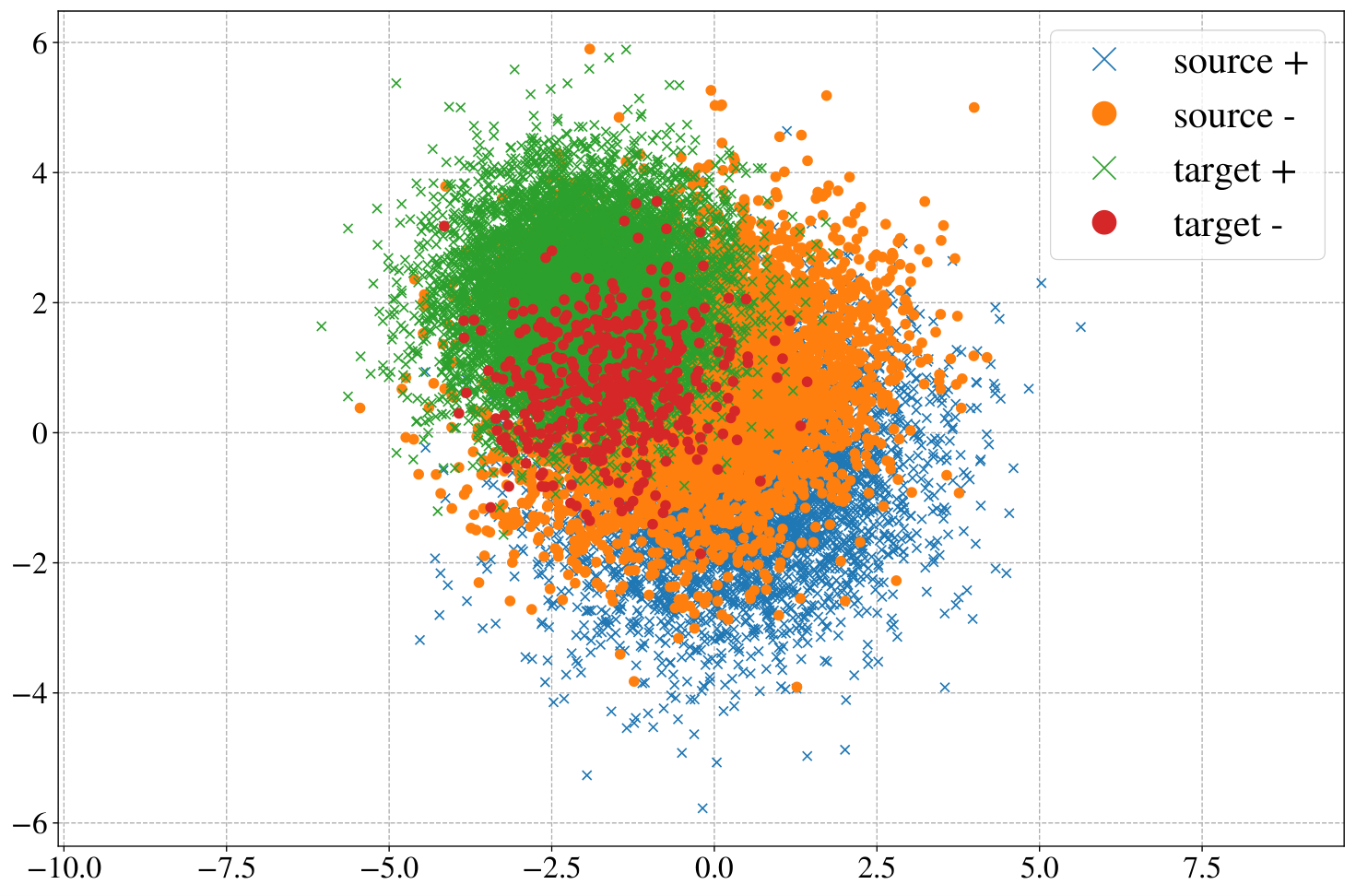
Here we truncate the Gaussian random variables $x_{i}=\{(x_{1},x_{2})\big|\|x_{1}\|_{2}<6,\|x_{2}\|_{2}<6\}$, for $i=1,\cdots,n$. We also restrict hypothesis space as $\mathcal{W}=\{w:\|w\|_{2}<3\}$ where $W_{{\sf{ERM}}}$ falls in this area with high probability. It can be easily checked that $\mu\ll\mu^{\prime}$ and the loss function is bounded, hence we can upper bound generalization error using Corollary 2. To this end, we firstly fix the source samples $n_{s}=10000$, while the target samples $n_{t}$ varies from 100 to 100000 and $\alpha=\beta=\frac{n_{t}}{n_{s}+n_{t}}$ following the guideline from [4, 6]. We give the empirical estimation for $r^{2}$ within the according hypothesis space such that

$\displaystyle r^{2}=\frac{\left(\max_{Z\in S^{\prime},w\in\mathcal{W}}{\ell(w,Z)}-\min_{Z\in S^{\prime},w\in\mathcal{W}}{\ell(w,Z)}\right)^{2}}{4}$

To evaluate the mutual information $I(W_{{\sf{ERM}}},Z_{i})$ efficiently, we follow the work [17] by repeatedly generating $W_{{\sf{ERM}}}$ and $Z_{i}$. As $\mu\ll\mu^{\prime}$ , we decompose $D(\mu(X,Y)\|\mu^{\prime}(X^{\prime},Y^{\prime}))=D(P_{X}\|P_{X^{\prime}})+\mathbb{E}_{X\sim P_{X}}\{D(P_{Y|X=x}\|P_{Y^{\prime}|X=x})\}$ in terms of the feature distributions and conditional distributions of the labels. The first term $D(P_{X}\|P_{X^{\prime}})$ can be calculated using the parameters of Gaussian distributions. The latter term denotes the expected KL-divergence over $P_{X}$ between two Bernoulli distributions, which can be evaluated by generating abundant samples from the source domain. Further we apply Theorem 2 to upper bound the excess risk, where we give a data-dependent estimation for the term $d_{\mathcal{W}}(\mu,\mu^{\prime})$ as

$\displaystyle\hat{d}_{\mathcal{W}}(\mu,\mu^{\prime})=\sup_{w\in\mathcal{W}}|\hat{L}(w,S)-\hat{L}(w,S^{\prime})|.$

To demonstrate the usefulness of our algorithm, we compare the bound in the following theorem using the Rademacher complexity under the same domain adaptation framework. Detailed experiment settings can be found in [12].

The comparisons of generalization error bound and excess risk bound are shown in figure 2. It is obvious that the true losses are bounded by our developed upper bounds. The result also suggests that our bound is tighter than Rademacher complexity bound in terms of both generalization error and excess risk. This is possibly due to that the generalization error bound with Rademacher complexity is characterized by the domain difference in the whole hypothesis space, while our bound is data-algorithm dependent, which is only concerned with $W_{{\sf{ERM}}}$. As expected, the data-algorithm dependent bound captures the true behaviour of generalization error while Rademacher complexity bound fails to do so. It is noteworthy that both bounds converge as $n$ increases. The result confirms that the bounds captures the dependence of the input data and output hypothesis, as well as the stochasticity of the algorithm.

References

- [1] D. Russo and J. Zou, “Controlling Bias in Adaptive Data Analysis Using Information Theory,” in Artificial Intelligence and Statistics, May 2016, pp. 1232–1240.
- [2] S. Shalev-Shwartz and S. Ben-David, Understanding Machine Learning by Shai Shalev-Shwartz. Cambridge Core, May 2014.
- [3] A. Asadi, E. Abbe, and S. Verdu, “Chaining Mutual Information and Tightening Generalization Bounds,” in Advances in Neural Information Processing Systems 31, S. Bengio, H. Wallach, H. Larochelle, K. Grauman, N. Cesa-Bianchi, and R. Garnett, Eds. Curran Associates, Inc., 2018, pp. 7234–7243.
- [4] S. Ben-David, J. Blitzer, K. Crammer, A. Kulesza, F. Pereira, and J. W. Vaughan, “A theory of learning from different domains,” Machine Learning, vol. 79, no. 1, pp. 151–175, May 2010.
- [5] J. Blitzer, K. Crammer, A. Kulesza, F. Pereira, and J. Wortman, “Learning Bounds for Domain Adaptation,” in Advances in Neural Information Processing Systems 20, J. C. Platt, D. Koller, Y. Singer, and S. T. Roweis, Eds. Curran Associates, Inc., 2008, pp. 129–136.
- [6] C. Zhang, L. Zhang, and J. Ye, “Generalization bounds for domain adaptation,” in Advances in neural information processing systems, 2012, pp. 3320–3328.
- [7] W. Dai, Q. Yang, G.-R. Xue, and Y. Yu, “Boosting for transfer learning,” in Proceedings of the 24th international conference on Machine learning. ACM, 2007, pp. 193–200.
- [8] Y. Zhang, T. Liu, M. Long, and M. I. Jordan, “Bridging theory and algorithm for domain adaptation,” arXiv preprint arXiv:1904.05801, 2019.
- [9] M. Long, J. Wang, G. Ding, S. J. Pan, and S. Y. Philip, “Adaptation regularization: A general framework for transfer learning,” IEEE Transactions on Knowledge and Data Engineering, vol. 26, no. 5, pp. 1076–1089, 2013.
- [10] A. Xu and M. Raginsky, “Information-theoretic analysis of generalization capability of learning algorithms,” in Advances in Neural Information Processing Systems 30, I. Guyon, U. V. Luxburg, S. Bengio, H. Wallach, R. Fergus, S. Vishwanathan, and R. Garnett, Eds. Curran Associates, Inc., 2017, pp. 2524–2533.
- [11] Y. Bu, S. Zou, and V. V. Veeravalli, “Tightening Mutual Information Based Bounds on Generalization Error,” arXiv:1901.04609 [cs, stat], Jan. 2019, arXiv: 1901.04609. [Online]. Available: http://arxiv.org/abs/1901.04609
- [12] “Supplementary materials - proofs.” [Online]. Available: https://github.com/wfyitf/Information-Theoretic-for-Domain-Adaptation/blob/master/Proof_ISIT2020.pdf
- [13] O. Bousquet and A. Elisseeff, “Stability and Generalization,” Journal of Machine Learning Research, vol. 2, no. Mar, pp. 499–526, 2002.
- [14] B. K. Sriperumbudur, K. Fukumizu, A. Gretton, B. Schölkopf, G. R. Lanckriet et al., “On the empirical estimation of integral probability metrics,” Electronic Journal of Statistics, vol. 6, pp. 1550–1599, 2012.
- [15] J. Jiao, Y. Han, and T. Weissman, “Dependence measures bounding the exploration bias for general measurements,” in 2017 IEEE International Symposium on Information Theory (ISIT), Jun. 2017, pp. 1475–1479.
- [16] M. Schmidt, N. L. Roux, and F. R. Bach, “Convergence rates of inexact proximal-gradient methods for convex optimization,” in Advances in neural information processing systems, 2011, pp. 1458–1466.
- [17] R. Moddemeijer, “On estimation of entropy and mutual information of continuous distributions,” Signal processing, vol. 16, no. 3, pp. 233–248, 1989.