Semi-online Scheduling: A Survey

We present three algorithmic frameworks such as offline, online and semi-online based on availability of input information in processing of a computational problem as shown in Figure 2.

• •

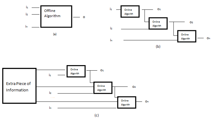
  In Offline framework, complete input information is known at the outset. Let us consider a set $I$=$\{i_{1},i_{2},...,i_{n}\}$ representing all inputs of a computational problem $X$. In offline framework, $I$ is known prior to construct a solution for $X$. The algorithm designed for computation of $I$ in the offline framework is known as offline algorithm. An offline algorithm processes all inputs $I$ simultaneously to produce the final output $o$.

• •

  In Online framework, the inputs are given one by one in order. Each available input must be processed immediately with no information on the successive inputs. In online framework, at the time step $t$, the input sequence $I_{t}$:$<i_{1},i_{2},...,i_{t-1},i_{t}>$ is known and must be processed irrevocably with no information on future input sequence $<i_{t+1},...,i_{n-1},i_{n}>$, where $t\geq 1$. The algorithm designed for computation of $I$ in the online framework is known as online algorithm. An online algorithm produces a partial output $o_{t}$ for each input $I_{t}$ on the fly, where, $1\leq t\leq n-1$ before producing the final output $o_{n}$.

• •

  In Semi-Online framework inputs are given one by one like online framework along with some Extra Piece of Information(EPI) on future inputs. At any time step $t$, a semi-online algorithm receives input sequence $I_{t}$ with an EPI and processes them irrevocably to obtain a partial output $o_{t}$ on the fly, where $1\leq t\leq n-1$ before producing the final output $0_{n}$.

Semi-online is an intermediate framework to address the practicability and limitations of online and offline frameworks. In most of the current practical scenarios, neither all the inputs are available at the beginning nor the inputs occur exclusively in online fashion, but may occur one by one with additional information on the successive inputs. For example, an online video on demand application receives requests for downloading video files on the fly, however, it knows the highly requested video file and the largest video file among all video files before processing the current request [79]. A related model to semi-online framework is the advice model, where the EPI has been referred to as bits of advice. A comprehensive survey on advice models can be found in [92].

Semi-online scheduling [13] is a variant of online scheduling with an EPI on future jobs or with additional algorithmic extensions by allowing two parallel policies to operate on each incoming job. It may also include a buffer of finite length for pre-processing of a newly arrived job before the actual assignment. We now formally define the semi-online scheduling problem by presenting inputs, constraints and output as follows.

• •

  Inputs:

  • –

    A sequence $J:<J_{1},J_{2}...,J_{n}>$ of $n$ jobs with corresponding processing time of $p_{i}$, where $1\leq i\leq n$ and $p_{i}>0$ are revealed one by one for processing on a list $M$=$(M_{1},M_{2},...,M_{m})$ of $m$ parallel machines, where $m\geq 2$ and $n>>>m$.

  • –

    An EPI such as arrival order of the jobs or largest processing time or upper and lower bounds on the processing time of the incoming jobs is given a priori.

• •

  Constraints:

  • –

    Each incoming job $J_{i}$ must be assigned irrevocably to one of the machines $M_{j}$ as soon as $J_{i}$ is given.

  • –

    Jobs are non-preemptive, however the preemptive variant of the problem supports job splitting to execute distinct pieces of a job at non-overlapping time spans on the same or different machines.

• •

  Output: Generation of a schedule, representing assignment of all jobs over $m$ machines.(we shall discuss about the output parameters and objectives in section 2.3).

Here, we discuss some of the important applications, where semi-online scheduling serves as a major algorithmic framework.

• •

  Resource Management in Operating System [2]: In a multi-user, time-shared operating system, it is not known at the outset the sequence of jobs or the number of jobs that would be submitted to the system. Here, jobs are given to the scheduler over time. However, it is the inherent property of the scheduler to make an educated guess about the maximum and minimum time required to complete a resident job. The objective is to irrevocably assign the required computer resources such as memory, processors immediately upon the availability of a job to attain a minimum completion time.

• •

  Distributed Data Management [15]: Distributed and parallel systems often confronted to store files of varying sizes on limited capacity remote servers. It is evident that files are submitted from a known source on the fly and each received file must be assigned immediately to one of the remote servers. The central scheduler of the system is handicapped about the successive submissions prior to make an irrevocable assignment. However, it is known for an instance that the submitting source stored the files in $k$ unit capacity servers, which provides a hint for the total size of files to be received. The challenge is to store the files on the remote servers with minimum storage requirement.

• •

  Server Request Management or Web Caching [40]: In a client-server model, it is not known in advance the number of requests that would be submitted to the remote servers nor the time required to process the requests. However, the hierarchical organizations of servers can serve as an extra piece of information for scheduler to cater different level of services to the requests with a broader objective of processing all requests as latest as possible.

• •

  Production and Manufacturing: Orders from clients arrive on the fly to a production system. The resources such as human beings, machinery equipment(s) and manufacturing unit(s) must be allocated immediately upon receiving each client order with no knowledge on the future orders. However, one could estimate the minimum or maximum time required to complete the order. Online arrival of the orders have high impact on the renting and purchasing of the high cost machines in the manufacturing units.

• •

  Maintenance and upgrade of industrial tools [52]: Scheduling of various maintenance and operational activities for modular gas turbine aircraft engines. The goal is to distribute different activities to the machines in such a way that the loads of the the machines will be balanced. The common practice is to maximize load of the least loaded machine.

Traditional techniques [17] for analyzing the performance of offline scheduling algorithms are largely relied on the entire job sequence, therefore are insignificant in the performance evaluation of semi-online algorithms, which operate on single incoming input at any given time step with minimal knowledge on the future arrivals.
Competitive analysis method [8] measures the worst-case performance of a semi-online algorithm $ALG$ designed either for a cost minimization or maximization problem by evaluating competitive ratio(CR). For a cost minimization problem, CR is defined as the smallest positive integer $k(\geq 1)$, such that for all valid sequences of inputs in the set $I$= $\{i_{1},i_{2},...,i_{n}\}$, we have $C_{ALG}\leq k\cdot C_{OPT}$, where $C_{ALG}$ is the cost obtained by semi-online algorithm $ALG$ for any sequence of $I$ and $C_{OPT}$ is the optimum cost incurred by the optimal offline algorithm $OPT$ for $I$. The Upper Bound(UB) on the CR obtained by $ALG$ guarantees the maximum value of CR for all legal sequences of $I$. The Lower Bound(LB) on the CR of a semi-online problem $X$ ensures that there exists an instance of $I$ such that any semi-online algorithm $ALG$ must incur a cost $C_{ALG}\geq b\cdot C_{OPT}$, where $b$ is referred to as LB for $X$. The performance of $ALG$ is considered to be tight, when $ALG$ ensures no gap between achieved LB and UB for the problem considered. Sometimes, the performance of $ALG$ is referred to as tight if $C_{ALG}$=$k\cdot C_{OPT}$. For a cost maximization problem, CR is defined as the infimum $k$ such that for any valid input sequence of $I$, we have $k\cdot C_{ALG}\geq C_{OPT}$. The objective of a semi-online algorithm is to obtain a CR as closer as possible to $1$(strictly greater than or equal to $1$).

Research in semi-online scheduling has been pioneered by the following non-trivial issues.

• •

  The offline $m$-machine($m\geq 2$) scheduling problem with makespan minimization objective has been proved to be NP-complete by a polynomial time reduction from well-known Partition problem [7]. Let us consider an instance of scheduling $n$ jobs on $m$ parallel machines, where $n>>>m$. There are $m^{n}$ possible assignments of jobs. An optimum schedule can be obtained in worst case with probability $\frac{1}{m^{n}}$. Further, unavailability of prior information about the whole set of jobs poses a non-trivial challenge in the design of efficient algorithms for semi-online scheduling problems.

• •

  Given an online scheduling problem considered in the semi-online framework, the non-trivial question raised is:
  What can be an additional realistic information on successive jobs that is necessary and sufficient to achieve $1$-competitiveness or to beat the best known bounds on the CR?

• •

  A semi-online algorithm is equivalent to an online algorithm with advice in the sense that an EPI considered in semi-online model can be encoded into bits of advice. The quantification of information into bits will help in analyzing the advice complexity of a semi-online algorithm. Any advancement in semi-online scheduling may lead to significant improvements in the best known bounds obtained by the advice models.

• •

  Semi-online model is practically significant than the advice model as it considers feasible information on future inputs unlike bits of advice, which sometimes may constitute an unrealistic information.

Scope. This paper surveys scholarly contributions in the design of semi-online scheduling algorithms in various parallel machine models such as identical and uniformly related by considering job’s processing formats such as preemptive and non-preemptive with the optimality criteria such as Min-Max and Max-Min. The aim of the paper is to record important competitive analysis results with the exploration of novel intuitions and critical ideas in a historical chronological overview.
Uniqueness. This is a comprehensive survey article on semi-online scheduling, which describes the motivation towards semi-online scheduling research, outlines a general taxonomy, states fifteen well-known semi-online scheduling algorithms, presents state of the art contributions, explains critical ideas, overviews important results in a chronological manner, organized by EPI considered in various semi-online scheduling setups. Several non-trivial research challenges and open problems are explored for future research work. Important references are grouped together in a single article to develop basic understanding, systematic study and to update the literature on semi-online scheduling for future investigation.

Parallel machine models support simultaneous execution of multiple threads of a single job or a number of jobs on $m$ machines, where $m\geq 2$. Semi-online scheduling problem has been studied in parallel machine models such as identical, uniformly related(or related machines in short) and unbounded batch machines. One model differs from another based on its processing power defined in the literature [6] as follows.

• •

  Identical Machines(P): Here, all machines have equal speeds of processing any job $J_{i}$. We have $p_{ij}=p_{i}$, $\forall M_{j},1\leq j\leq m$.

• •

  Related Machines (Q): Here, the machines operate at different speeds. For a machine $M_{j}$ with speed $S_{j}$, execution time of job $J_{i}$ on $M_{j}$ is $p_{ij}=\frac{p_{i}}{S_{j}}$.

• •

  Unbounded Batch Machine (U-batch): A batch machine receives jobs in batches, where a batch($U(t)$) is formed by considering all jobs that are received at time $t$. The jobs in $U(t)$ are processed at the same time in the sense that the completion time($U(c_{t})$) of all jobs in a batch are same. The processing time of $U(t)$ is $U(p_{t})$=$\max\{p_{1},p_{2},...,p_{k}\}$ and the completion time $U(c_{t})$=$t+U(p_{t})$, where $k$ is the size of $U(t)$ i.e. the number of jobs in a batch. When the size of the batches are not bounded with any positive integers, then it is called unbounded batch machine with $k$=$\infty$.

Job characteristics describe the nature of the jobs and related characteristics to job scheduling [6, 49]. All jobs of any scheduling problem must possess at least one of the characteristics specified in set $\beta=\{\beta_{1},\beta_{2},\beta_{3},\beta_{4},\beta_{5}\}$. In semi-online scheduling, a new job characteristic $\beta_{6}$ is introduced to represent extra piece of information(EPI) on future jobs. The job characteristics are presented as follows: $\beta_{1}$ specifies whether preemption or job splitting is allowed, $\beta_{2}$ specifies precedence relations or dependencies among the jobs, $\beta_{3}$ specifies release time for each job, $\beta_{4}$ specifies restrictions related to processing times of the jobs, for example, if $\beta_{4}$=$1$, that means $p_{i}=1$, $\forall J_{i}$, $\beta_{5}$ specifies deadline($d_{i}$) for each job $j_{i}$, indicating the execution of each $j_{i}$ must be finished by time $d_{i}$, otherwise an extra penalty may incur due to deadline over run. Let us throw more clarity on some of the important job characteristics as follows.
Preemption(pmtn) allows splitting of a job into pieces, where each piece is executed on the same or different machines in non-overlapping time spans.
Non-preemption(N-pmtn) ensures that once a job $J_{i}$ with processing time $p_{i}$ begins to execute on machine $M_{j}$ at time $t$, then $J_{i}$ continues the execution on $M_{j}$ until time $t+p_{i}$ with no interruption in between.
Precedence Relation defines dependencies among the jobs by the partial order ’$\prec$’ rule on the set of jobs [5]. A partial order can be defined on two jobs $J_{i}$ and $J_{k}$ as $J_{i}$ $\prec$ $J_{k}$, which indicates execution of $J_{k}$ never starts before the completion of $J_{i}$. The dependencies among different jobs can be illustrated with a precedence graph $G(p,\prec)$, where each vertex represents a job $J_{i}$ and labeled with its processing time $p_{i}$. A directed arc between two vertices in $G(p,<)$ i.e $J_{i}$ $\rightarrow$ $J_{k}$ represents $J_{i}$ $\prec$ $J_{k}$, where $J_{i}$ is referred to as predecessor of $J_{k}$. If there exists a cycle in the precedence graph, then scheduling is not possible for the jobs. When there is no precedence relation defined on the jobs, then they are said to be independent. We represent precedence relation among the jobs through precedence graphs by considering three jobs $J_{1}$, $J_{2}$, $J_{3}$ and their dependency relations as shown in Figure 4.

Extra Piece of Information(EPI) is the additional information given to an online scheduling algorithm about the future jobs. Motivated by the interactive applications, a number of EPIs have been considered in the literature(see the recent surveys [92], [108]) to gain a significant performance improvement over the pure online scheduling policies [92]. We now present the definitions and notations of some well studied EPIs as follows.

• •

  Sum(T). $\sum_{i=1}^{n}{p_{i}}$ Total size of all jobs [13].

• •

  Max($p_{max}$). $\max\{p_{i}|1\leq i\leq n\}$ Largest processing time or largest size job [20].

• •

  Optimum Makespan(Opt). Value of the optimum makespan is often represented by the following two general bounds [15].
           $C_{OPT}\geq\frac{1}{m}\cdot\sum_{i=1}^{n}{p_{ij}}$    and
           $C_{OPT}\geq p_{max}$.

• •

  Tightly Grouped Processing time (TGRP). Lower and upper bounds on the processing times of all jobs [20]. Some authors [22, 31, 45] considered either lower bound TGRP(lb) or upper bound TGRP(ub) on the processing times of the jobs.

• •

  Arrival Order of Jobs. $p_{i+1}\leq p_{i}$, for $1\leq i\leq n$ Jobs arrive, in order of non-incresing sizes (Decr) [21] or $r_{i+1}\geq r_{i}$ in order of non-decreasing release times (Incr-r) [70,87].

• •

  Buffer(B(k)). A buffer (B(k)) is a storage unit of finite length $k$($\geq 1$), capable of storing at most $k$ jobs [13]. The weight of B(k) is $w(B(k))\leq\sum_{i=1}^{k}{p_{i}}$. Availability of buffer allows an online scheduling algorithm either to keep an incoming job temporarily in the buffer or to irrevocably assign a job to a machine in case the buffer is full [13]. Therefore, information about $k+1$ future jobs is always known prior to make an efficient scheduling decision. The following variations in the buffer length and usage of buffer have been explored in the literature: buffer with length $k$($\geq 1$) i.e B(k) [13], buffer with length 1 i.e B(1) [13, 14] and re-ordering of buffer presented as re B(k) [56].

• •

  Information on Last Job. It is known in advance that last job has the largest processing time i.e. $p_{n}$=$p_{max}$, this EPI is denoted by LL in [26]. In [28], it is considered that several jobs arrive at the same as last job and this EPI is denoted by Sugg.

• •

  Inexact Partial Information. Inexact partial information is also referred to as disturbed partial information, which deals with the scenario, where the extra piece of information available to the online algorithm is not exact. For example, the algorithm knows a nearest value of the actual Sum but not the exact value. This EPI is represented as $disSum$ in [53].

• •

  Reassignment of Jobs($reasgn$). Once all jobs are assigned to the machines, again they can be reallocated to different machines with some pre-defined conditions. Several conditions on reassignment policies have been proposed in the literature [57, 62] such as reassign the last $k$ jobs, we represent as $reasgn(last(k))$, reassign arbitrary $k$ jobs i.e. $reasgn(k^{*})$, reassign only the last job of all machines i.e. $reasgn{(last)}^{*}$, reassign last job of any one of the machines, represented by $reasgn({(last)}^{1})$.

• •

  Machine availability ($mchavl$). All machines may not available initially. Machines are available on demand and the release time ($r_{j}$) of machine $M_{j}$ is known in advance [64]. Some authors have also considered the scenario where one machine is available for all jobs and other machine is available for few designated jobs [82].

• •

  Grade of Service (GOS) or Machine Hierarchy. It is known a priori that machines are arranged in a hierarchical fashion to cater different levels of services to the jobs with some defined GOS [36, 46]. For example, if a GOS of $g_{2}$ is defined for any job $J_{i}$, then $J_{i}$ can only be assigned to machine $M_{2}$ and if $J_{i}$ has GOS of $g_{1}$, then it can be scheduled on any of the machines.

Several optimality criteria or output parameters have been investigated in the offline and online settings [17, 49]. However, in semi-online scheduling the following output parameters have been considered mostly: makespan and load balancing.

• •

  Makespan($C_{max}$) represents completion time($c_{i}$) of the job that finishes last in the schedule, $C_{max}$=$\max\{c_{i}|1\leq i\leq n\}$ or $C_{max}$=$\min\{l_{j}|1\leq j\leq m\}$. The objective is to minimize $C_{max}$, otherwise termed as minimization of the load of highest loaded machine(min-max).

• •

  Load Balancing describes the objective to maximize the minimum machine load(max-min) or machine cover. The scheduler assigns certain number of jobs to each machine for the processing of $n$ jobs on $m$ machines. Each job $J_{i}$ adds $p_{i}$ amount of load to the assigned machine $M_{j}$. The goal is to maximize the minimum load occurs on any of the machines so as to keep a balance in the incurred loads among all machines. We refer $C_{min}$ to represent max-min objective. As an example, Figure 5 shows the loads of machines during the processing of a specified number of jobs.

Examples: We present various semi-online scheduling setups based on the three fields ($\alpha|\beta|\gamma$) classification format as shown in Table 2.

Buffer, Sum. Kellerer et al. [13] envisioned semi-online scheduling as a theoretically significant and practically well performed online scheduling model. They initiated the study on semi-online scheduling by considering Sum as the known EPI and proposed algorithm $H_{3}$ for the setup $P_{2}|Sum|C_{max}$. Algorithm $H_{3}$ outperforms algorithm LS and achieves a tight bound $1.33$ for $m=2$. To show the LB $1.33$ of algorithm $H_{3}$, let us consider an instance of $P_{2}|Sum|C_{max}$, where $Sum$=$2$. Algorithm $H_{3}$ schedules each incoming job $J_{i}$ to machine $M_{1}$ until $l_{1}+p_{i}\leq\frac{2}{3}\cdot$(Sum) and assigns the remaining jobs to machine $M_{2}$. If we consider $Sum$=$2$, then irrespective of the input instances, the final loads $l_{1}$, $l_{2}$ would be $\frac{4}{3}$, $\frac{2}{3}$ respectively and $C_{OPT}$ would be $1$. This implies, $C_{H_{3}}\geq 1.33\cdot(C_{OPT})$. The semi-online strategy of Kellerer et al. unveils that advance knowledge of Sum helps any online algorithm $A$ to schedule incoming jobs to a particular machine until its load reaches upto a judiciously chosen fraction of the Sum and assigns the remaining jobs to the other machine such that the ratio between $C_{A}$ and $C_{OPT}$ results in the improved competitive bound. They also studied semi-online scheduling with a buffer($B$) of length $k$ and proposed algorithm $H_{1}$ for the setup $P_{2}|B(k)|C_{max}$. They proved that any online scheduling algorithm with $B(k)$ achieves a CR of at least $1.33$. The LB can be shown by considering an online sequence $J:<J_{1}/1,J_{2}/1,J_{3}/1,J_{4}/3>$ of four jobs with specified processing times and $k$=$1$. Algorithm $H_{1}$ keeps the first available job $J_{1}$ in the buffer. Thereafter, each incoming $J_{i+1}$, where $1\leq i\leq 3$, is either kept in the buffer or any $J_{x}\in\{J_{i},J_{i+1}\}$ is scheduled on machine $M_{1}$ if $l_{1}+p_{x}\leq\frac{2}{3}\cdot(l_{1}+l_{2}+w(B))$, else any $J_{x}$ is assigned to machine $M_{2}$ (Note that $w(B)$=$p_{i}+p_{i+1}$). We now have a schedule due to algorithm $H_{1}$ with the sequence of assignments of $J$ on the machines as follows: $J_{1}/1$ on $M_{1}$, $J_{2}/1$ on $M_{2}$, $J_{4}/3$ on $M_{1}$ and $J_{3}/1$ on $M_{2}$ such that $C_{H_{1}}\geq 4$, where $C_{OPT}\geq 3$. Therefore, $C_{H_{1}}\geq 1.33\cdot(C_{OPT})$. A matching UB was shown to achieve a tight bound $1.33$ for algorithm $H_{1}$. They also studied a semi-online variant, where two parallel processors are given to virtually schedule a sequence of incoming jobs over $2$-identical machines by two distinct procedures independently. Finally, the jobs are scheduled by the procedure that has incurred minimum $C_{max}$ for the entire job sequence. They obtained a tight bound $1.33$ for the semi-online variant $P_{2}|2$-$Proc|C_{max}$. Zhang [14] studied the setup $P_{2}|B(1)|C_{max}$ and obtained the tight bound $1.33$ with an alternate policy. The policy keeps the first job $J_{1}$ in the buffer and if no further jobs arrive, then $J_{1}$ is scheduled on machine $M_{2}$, else for next incoming job $J_{i+1}$, where $1\leq i\leq n-1$, the job $J_{x}$ is chosen from $\{J_{i},J_{i+1}\}$ such that $p_{x}$ is minimum (let us denote the other job as $J_{y}$). Now, $J_{x}$ is assigned to machine $M_{1}$ if $l_{1}+p_{x}\leq 2\cdot(l_{2}+p_{y})$, else $J_{x}$ is scheduled on machine $M_{2}$. If there is no jobs to arrive further, then the last job in the buffer is assigned to machine $M_{2}$. The aim of the policy is to keep a larger load difference between machines $M_{1}$ and $M_{2}$ by assigning smaller jobs to $M_{2}$ such that at any time step, the availability and assignment of an unexpected larger job would not incur a makespan beyond $1.33\cdot(C_{OPT})$. Angelelli [22] proposed an alternative to algorithm $H_{3}$ [13] as algorithm H for $P_{2}|Sum|C_{max}$ and obtained tight bound $1.33$. He analyzed the performance of algorithm H by considering various ranges of lower bounds on the processing times of the jobs. Girlich et al. [18] obtained an UB $1.66$ for $P_{m}|Sum|C_{max}$.
TGRP, Max. He and Zhang [20] initiated study on the setup $P_{2}|TGRP|C_{max}$ by assuming that all jobs have processing times within the interval of $p$ and $rp$, where $p>0$ and $r\geq 1$. They proved that any online algorithm $A$ must have $C_{A}\geq\frac{r+1}{2}$ for $r\leq 2$ and $C_{A}\geq 1.5$ for $r>2$. They analyzed algorithm LS for $P_{m}|TGRP|C_{max}$ and showed that $C_{LS}\leq(1+\frac{(m-1)(r-1)}{m})\cdot C_{OPT}$. They obtained LB $1.33$ for the setup $P_{2}|Max|C_{max}$ by considering the online availability of the job sequence $J:<J_{1}/1,J_{2}/1,J_{3}/2,J_{4}/2>$, where $p_{max}$=$2$ is known a priori. Following the optimum policy [2] of keeping a machine free for the largest job and assigning the sequence of comparatively shorter jobs to the remaining machines, any online algorithm $A$ assigns $J_{1}/1$ and $J_{2}/1$ on $M_{1}$ followed by the assignments of $J_{3}/2$ on $M_{2}$ and $J_{4}/2$ on either $M_{1}$ or $M_{2}$ to incur $C_{A}\geq 4$, where $C_{OPT}\geq 3$. This implies $C_{A}\geq 1.33\cdot(C_{OPT})$. They proposed algorithm PLS to achieve a tight bound $1.33$. Algorithm PLS always maintains a load difference maximum of upto $p_{max}$ between machines $M_{1}$ and $M_{2}$ such that scheduling of the largest job on the smallest loaded machine almost equalizes the loads of both the machines.
Opt. Azar and Regev [15] introduced a variant of the classical bin-stretching problem, where items are available one by one in order and each available item must be packed into one of the $m$ bins before the availability of the next item. It is known apriori that all items can be placed into $m$ unit sized bins. The goal is to stretch the bins as minimum as possible so as to fit all items into the bins. Therefore, the bin stretching problem considered by Azar and Regev is analogous to the setup $P_{m}|Opt|C_{max}$. They achieved an UB $1.625$ for large $m$. The key idea is to first define the threshold values $\alpha$ and $2\alpha-1$ based on the value of known Opt. Then, arrange $m$ machines in at least two distinct sets based on their loads with respect to $\alpha$ and $2\alpha-1$. A new job is now assigned to the selected machine belongs to the chosen set. Improved rules can be defined for the selections of set and machine. Here, a non-trivial challenge is to define and characterize the threshold values.
Decr and Preemptive Semi-online Scheduling. Seiden et al. [21] analyzed algorithm LPT [3] with known Decr and achieved a tight bound $1.166$ for $m$=$2$ and LB $1.18$ for $m$=$3$. They initiated the study on $P_{m}|pmtn,Decr|C_{max}$ and obtained tight bound $1.366$. They assumed preemption as job splitting for scheduling distinct pieces of an incoming job in the non-overlapping time slots. To understand the notion of job splitting, let us consider a sequence of jobs of unit sizes. Suppose, the required CR to be obtained is $k$. Now, the initial $m$ incoming jobs are splitted into at most two pieces each such that all pieces of a job execute in distinct time slots and all jobs are finished by time $k$. Let $r$=$\lfloor\frac{m}{k}\rfloor$, $i\leq r$, each incoming job $J_{m+i}$ is splitted and assigned to the first $i$ machines such that each machine gets $\frac{k}{m}$ fraction of the processing time of job $J_{m+i}$ and its remaining fraction is assigned prior to time $k$. We now have $i$ highest loads of the machines represented as: $k(1+\frac{i}{m})$, $k(1+\frac{i-1}{m})$,…,$k(1+\frac{1}{m})$, which ensures non-overlapping time slots in the subsequent rounds. Similarly, the next jobs followed by the $({m+r})^{th}$ job are scheduled only in the time slots after $k$ on at most $r+1$ machines. A non-trivial challenge is to rightly choose the values of $r$ and $k$ such that the load to be scheduled prior to time $k$ is at most $k\cdot m$. The authors conjectured that the achieved tight bound $1.366$ with known Decr can possibly be achieved with only known $p_{max}$. Further, they showed that randomization in scheduling decision making does not lead to improved the CR for the setup $P_{m}|pmtn,Decr|C_{max}$. We now present the main results obtained for semi-online scheduling in identical machines for the years 1997-2000 in table 3.

During the years 2001-2005, semi-online scheduling was studied not only for identical machines but for uniform related machines as well. Both preemptive and non-preemptive processing formats were investigated. The concept of combined EPI and a new EPI on the last job were introduced. We present the state of the art contributions in semi-online scheduling for related machines and identical machines as follows.

Related Machines:
Decr. Tan and He [23] proposed algorithm Ordinal for non-preemptive semi-online scheduling with ordinal data [11] and known Decr for $2$-uniformly related machines, where $S_{1}$=$1$ and $S_{2}\geq 1$. They analyzed and proved competitiveness of the algorithm as an interval wise function of machines’ speed ratio $s$. They proved the tightness of the algorithm in most of the intervals of $s\in[1,\infty)$. As a main result, they produced UB $\frac{s+1}{s}$ for $s\geq 2.732$ and LB $\frac{s+1}{s}$ for $s\in[2.732,\infty)$. However, the LB of algorithm Ordinal does not match with its UB when the total length of the speed ratio interval reduces to $0.7784$, where the largest gap between the intervals is at most $0.0521$. Epstein and Favrholdt [30] initiated study on the setup $Q_{2}|pmtn,Decr|C_{max}$ and achieved competitive ratios of $\frac{3(s+1)}{3s+2}$ for $1\leq s\leq 3$ and $\frac{2s+(s+1)}{2s^{2}+s+1}$ for $s\geq 3$. In [42], they investigated the setup $Q_{2}|Decr|C_{max}$, where $S_{1}$=$1$ and $S_{2}$=$\frac{1}{s}$. They expressed competitive ratios as a function of $15$ speed ratio intervals. They proposed algorithm ELPT and achieved tight bound $1.28$ for $s$=$1.28$. They proposed algorithm Slow-LPT for $s\in[1,\frac{1}{6}(1+\sqrt{37})]$ and obtained a tight bound $1.28$. Here, the key idea is to initially use the slowest machine and keep the fastest machine free for incoming larger jobs. They proposed algorithms Balanced-LPT and Opposite-LPT for the remaining intervals, where algorithms ELPT and Slow-LPT do not obtain tight bounds. Algorithm Balanced-LPT schedules the first job $J_{1}$ on the fastest machine $M_{1}$. The second job $J_{2}$ is assigned to machine $M_{2}$ if $s>c(s)(p_{1}+p_{2})$, else job $J_{2}$ is scheduled on $M_{1}$, where $c(s)$=$2.19$ for $s\in[2,2.19]$ and $c(s)$=$2.57$ for $s\in[2.35,2.57]$. Thereafter, remaining jobs are scheduled by algorithm ELPT. Algorithm Opposite-LPT also schedules job $J_{1}$ on machine $M_{1}$. The second job $J_{2}$ is scheduled on $M_{1}$ if $s\cdot p_{2}<(p_{1}+p_{2})\leq c(s)\cdot s\cdot p_{2}$, else $J_{2}$ is scheduled on $M_{2}$, where $c(s)$=$2.35$ for $s\in[2.19,2.35]$. Thereafter, the subsequent jobs are scheduled by the ELPT rule.
Opt. Epstein [33] studied semi-online scheduling for the setup $Q_{2}|Opt|C_{max}$, where $S_{1}$=$1$ and $S_{2}$=$\frac{1}{s}$. He proposed algorithm SLOW by considering $C_{OPT}$=$1$ and $s\geq\sqrt{2}$. Algorithm SLOW schedules an incoming job $J_{i}$ to machine $M_{1}$ if $l_{2}\geq\frac{1}{s^{2}+s}$; else if $l_{2}+p_{j}\geq\frac{C_{SL}(s)}{s}$, then job $J_{i}$ is assigned to machine $M_{2}$; else $J_{i}$ is scheduled on machine $M_{1}$, where $C_{SL}(s)$=$\frac{s+2}{s+1}$. Algorithm SLOW performs better in the scenario, where the slowest machine $M_{2}$ is relatively very slow and initial jobs needs to be assigned to it for keeping the high speed machine $M_{1}$ relatively free for future larger jobs. For $s\leq\sqrt{2}$, Epstein proposed algorithm FAST by considering $C_{OPT}$=$1$. Algorithm FAST assigns an incoming job $J_{i}$ to machine $M_{2}$ if a job $J_{x}$ was earlier assigned to $M_{2}$ due to $l_{1}<(1+\frac{1}{s}-\frac{C_{FA}(s)}{s})$ and $(l_{1}+p_{x})>C_{FA}(s)$; else if $l_{1}\geq(1+\frac{1}{s}-\frac{C_{FA}(s)}{s})$, then $J_{i}$ is scheduled on $M_{2}$; else if $(l_{1}+p_{j})\leq C_{FA}(s)$, then $J_{i}$ is scheduled on $M_{1}$; else $J_{i}$ is assigned to machine $M_{2}$, where $C_{FA}(s)$=$\frac{2s+2}{2s+1}$ for $1\leq s\leq\frac{1+\sqrt{17}}{4}$ and $C_{FA}(s)$=$s$ for $\frac{1+\sqrt{17}}{4}\leq s\leq\sqrt{2}$. Algorithm FAST performs better in the cases, where the slowest machine $M_{2}$ is considerably fast, thus allowing initial jobs to be scheduled on the fastest machine $M_{1}$. He achieved lower bounds in terms of function of defined speed ratio intervals and obtained overall CR of $1.414$ and LB of $1.366$.
TGRP, Max. He and Jiang [34] studied the setup $Q_{2}|pmtn,TGRP(p,xp)|C_{max}$ by considering $S_{1}$=$1$ and $S_{2}\geq 1$, where $p>0$ and job size ratio $x\geq 1$. They initiated analysis of algorithm with respect to speed ratio intervals ($s\geq 1$) and job size ratios. They achieved a tight bound $\frac{s^{2}+s}{s^{2}+1}$ for $s\geq 1$ and $x<2s$. For $s\geq 1$ and $x\geq 2s$, the tight bound $\frac{1+2s+s^{2}}{1+s+s^{2}}$ was obtained. Further, they investigated the setup $Q_{2}|pmtn,Max|C_{max}$ by considering known $p_{max}$=$s\geq 1$. They achieved a CR of $\frac{2s^{2}+3s+1}{2s^{2}+2s+1}$ for $s\geq 1$. They explored that information on Max is weaker than known Decr for preemptive semi-online scheduling on $2$-related machine. We now present the main results obtained for semi-online scheduling on related machines for the years 2001-2005 in table 4.

References

- [1] R. McNaughton. Scheduling with deadlines and loss functions. Management Science, vol. 6, no. 1, pp. 1-12, 1959.
- [2] R. L. Graham. Bounds for certain multiprocessing anomalies. Bell system Technical Journal 45, pp. 1563-1581, 1966.
- [3] R. L. Graham. Bounds on multiprocessor timing anomalies. SIAM Journal of Applied Mathematics, vol. 17, no. 2, pp. 416-429, 1969.
- [4] R. W. Conway, W. L. Maxwell, L. W. Miller. Theory of Scheduling, Addison-Wesley, Reading, 1967.
- [5] K. R. Baker. Introduction to sequencing and scheduling, Wiley, New York, 1974.
- [6] R. L. Graham, E. L. Lawer, J. K. Lenstra, A. H. Rinnooy Kan. Optimization and approximation in deterministic sequencing and scheduling : A Survey. Annals of Discrete Mathematics 5, pp. 287-326, 1979.
- [7] M. R. Garey, D. S. Johnson. Computers and Intractability: A Guide to the Theory of NP-Completeness. Freeman, 1979.
- [8] R. E. Tarjan and S. Sleator. Amortized computational complexity. SIAM Journal on Algebraic and Discrete Methods, vol. 6, no. 2, pp. 306-318, 1985.
- [9] U. Faigle, W. Kern, G. Turan. On the performance of online algorithms for partition problems. Acta Cybernetica 9, pp. 107-119, 1989.
- [10] Y. Azar, J. Naor, R. Rom. The competitiveness of on-line assignments. Journal of Algorithms, vol. 18 no. 2, pp. 221-237, 1995.
- [11] W. P. Liu, J. B. Sidney, A. Vliet. Ordinal algorithms for parallel machine scheduling. Operations Research Letters 18, pp. 223-232, 1996.
- [12] D. B. Shmoys, J. Wein, D. P. Williamson. Scheduling parallel machines online. SIAM Journal on computing 24, pp. 1313-1331, 1995.
- [13] H. Kellerer, V. Kotov, M. G. Speranza, T. Tuza. Semi-online algorithms for the partition problem. Operations Research Letters 21, pp. 235-242, 1997.
- [14] G. Zhang. A simple semi-online algorithm for with a buffer. Information Processing Letters 61, pp. 145-148, 1997.
- [15] Y. Azar, O. Regev. On-line bin-stretching. In International Workshop on Randomization and Approximation Techniques in Computer Science(RANDOM), pp. 71-81. Springer, Berlin, Heidelberg, 1998.
- [16] J. Sgall. Online Scheduling: A survey. Lecture Notes in Computer Science, Springer 1442, pp. 196-231, 1998.
- [17] B. Chen, C. N. Potts, G. J. Woeginger. A review of Machine Scheduling: Complexity, Algorithms and Approximability. Handbook of Combinatorial Optimization 3, pp. 21-169, Kluwer Academic Publishers, 1998.
- [18] E. Girlich, V. Kotov, M. Kovalev. Semi-online algorithm for multiprocessor scheduling problem with a given total processing time. Technical Report 98-05, the Mathematical department, University Magdeburg, Germany, 1998.
- [19] C. Imreh, J. Noga. Scheduling with machine cost. In Proceedings of ESA’99, Lecture notes in Computer Science, Springer-Verlag, pp. 168-176, 1999.
- [20] Y. He, G. Zhang. Semi-online scheduling on two identical machines. Computing 62, pp. 179-187, Springer-Verlag, 1999.
- [21] S. Seiden, J. Sgall, G. Woeginger. Semi-online scheduling with decreasing job sizes. Operations Research Letters 27, pp. 215-221, 2000.
- [22] E. Angelelli. Semi-online scheduling on two parallel processors with known sum and lower bound on the size of the tasks. Central European Journal of Operations Research 8, pp. 285-295, 2000.
- [23] Z. Tan, Y. He. Semi-online scheduling with ordinal data on two uniform machines. Operations Research Letters 28, pp. 221-231, 2001.
- [24] H. Yong. Semi-online scheduling problems for maximizing the minimum machine completion time. Acta Mathematica App. sin., vol. 17, no. 1, 2001.
- [25] G. Zhang, X. Cai, C. K. Wong. Online algorithms for minimizing makespan on batch processing machines. Naval Research Logistics 48, pp. 241-258, 2001.
- [26] G. Zhang , Ye. Deshi. A note on on-line scheduling with partial information. Computers and Mathematics with Application 44, pp. 539-543, 2002.
- [27] H. He, C. Cai. Semi-online scheduling with machine cost. Journal of Computer Science and Technology, vol. 17, no. 6, 2002.
- [28] Z. Tan, Y. He. Semi-online problems on two identical machines with combined partial information. Operations Research Letters 30, pp. 408-414, 2002.
- [29] S. Y. Cai. Semi-online scheduling on 3 identical machines. Journal of Wenzhou Teachers College 23, pp. 1-3(in chinese), 2002.
- [30] L. Epstein, L. Favrholdt. Optimal preemptive semi-online scheduling to minimize makespan on two related machines. Operations Research Letters 30, pp. 269-275, 2002.
- [31] E. Angelelli, M. G. Speranza, Z. Tuza. Semi-online scheduling on two parallel processors with an upper bound on items. Algorithmica 37, pp. 243-262, Springer-Verlag, 2003.
- [32] X. Deng, C. K. Poon, Y. Zhang. Approximation algorithm in batch processing. Journal of Combinatorial Optimization, vol. 7, no. 3, pp. 247-257, 2003.
- [33] L. Epstein. Bin stretching revisited. Acta Informatica, vol. 39, no. 2, pp. 97-117, 2003.
- [34] Y. He, Y. Jiang. Optimal algorithms for semi-online preemptive scheduling problems on two uniform machines. Acta Informatica, vol. 40, no. 5, pp. 367-383, 2004.
- [35] E. Angelelli, A. B. Nagy, M. G. Speranza, Z. Tuza. The online multiprocessor scheduling problem with known sum of the tasks. Journal of Scheduling, vol. 7, no. 6, pp. 421-428, 2004.
- [36] H. Hwang, S. Chang, K. Lee. Parallel machine scheduling under a grade of service provision. Computers and Operations Research 31, pp. 2055-2061, 2004.
- [37] G. Dosa, Y. He. Semi-online algorithms for parallel machine scheduling problems. Computing 72, pp. 355-363, 2004.
- [38] R. Li, He. Huang. Online scheduling of jobs with arbitrary release times. Computing 73, pp. 79-97, 2004.
- [39] J. Krokowski, H. Racke, C. Sohler, M. Westermann. Reducing state changes with a pipeline buffer. In Proceedings of the International Fall Workshop Vision, Modeling, and Visualization (VMV), pp. 217-224, 2004.
- [40] T. Feder, R. Motwani, R. Panigrahi, S. Seiden, R. van Stee, A. Zhu. Combining request scheduling with web caching. Theoretical Computer Science, vol. 324, no. 23, pp. 201-218, 2004.
- [41] K. Pruhs, J. Sgall and E. Torng. Online scheduling. Handbook on scheduling: Algorithms, models and performance analysis, CRC Press, 2004
- [42] L. Epstein, L. M. Favrholdt. Optimal non-preemptive semi-online scheduling on two related machines. Journal of Algorithms 57, pp. 49-73, 2005.
- [43] Y. He, G. Dosa. Semi-online scheduling jobs with tightly grouped processing times on three identical machines. Discrete Applied Mathematics 150, pp. 140-159, 2005.
- [44] T. C. E. Cheng, H. Kellerer, V. Kotov. Semi-online multiprocessor scheduling with given total processing time. Theoretical Computer Science 337, pp. 134-146, 2005.
- [45] E. Angelelli, M. G. Speranza, Z. Tuza. New bounds and algorithms for online scheduling: two identical processors, known sum and upper bound on the task. Discrete Mathematics and Theoretical Computer Science 8, pp. 1-16, 2006.
- [46] J. Park, S. Y. Chang, K. Lee. Online and semi-online scheduling of two machines under a grade of service provision. Operations Research Letters 34, pp. 692-696, 2006.
- [47] Y. Jiang, Y. He, C. Tang. Optimal online algorithms for scheduling on two identical machines under a grade of service. Journal of Zhejiang University-Science A, vol. 7, no. 3, pp. 309-314, 2006.
- [48] R. Hua, J. Hu, L. Lu. A semi-online algorithm for parallel machine scheduling on three machines. Journal of Industrial Engineering and Management 20, 2006 (in Chinese).
- [49] P. Brucker. Scheduling Algorithms. Book edition, Springer, 2006.
- [50] E. Angelelli, M. G. Speranza, Z. Tuza. Semi on-line scheduling on three processors with known sum of the tasks. Journal of Scheduling, vol. 10, no. 4-5, pp. 263-269, 2007.
- [51] L. Epstein, D. Ye. Semi-online scheduling with end of sequence information. Journal of Combinatorial Optimization, vol. 14, no. 1, pp. 45-61, 2007.
- [52] Z. Tan, Y. Wu. Optimal semi-online algorithms for machine covering. Theoretical Computer Science 372, pp. 69-80, 2007.
- [53] Z. Tan, Y. He. Semi-online scheduling problems on two identical machines with inexact partial information. Theoretical Computer Science 377, pp. 110-125, 2007.
- [54] Y. Wu, Z. Tan, Q. Yang. Optimal semi-online scheduling algorithms on a small number of machines. Lecture Notes in Computer Science 4614, pp. 504-515, 2007.
- [55] E. Angelelli, M. G. Speranza, Z. Tuza. Semi-online scheduling on two uniform processors. Theoretical Computer Science 393, pp. 211-219, 2008.
- [56] M. Englart, D. Ozmen, M. Westermann. The power of re-ordering for online minimum makespan scheduling. Annual IEEE symposium on Foundations of Computer Science(FOCS), 2008.
- [57] Z. Y. Tan, S. H. Yu. Online scheduling with reassignment. Operations Research Letters, vol. 36, no. 2, pp. 250-254, 2008.
- [58] Y. Wu, Y. Huang, Q. F. Yang. Semi-online multiprocessor scheduling with the longest given processing time. Journal of Zhejiang University Science Edition 35, pp. 23-26, 2008 (in Chinese).
- [59] O. Chassid, L. Epstein. The hierarchical model for load balancing on two machines. Journal of Combinatorial Optimization, vol. 15, no. 4, pp. 305-314,2008.
- [60] C. T. Ng, Z. Tan, Y. He, T. C. E Cheng. Two semi-online scheduling problems on two uniform machines. Theoretical Computer Science, 410, pp. 776-792, 2009.
- [61] T. Ebelendr, J. Sgall. Semi-online preemptive scheduling: one algorithm for all variants. Symposium on Theoretical Aspects of Computer Science, pp. 349-360, 2009.
- [62] M. Liu, Y. Xu, C. Chu, F. Zhang. Online scheduling on two uniform machines to minimize the makespan. Theoretical Computer Science 410(21-23), pp. 2099-2109, 2009.
- [63] E. Angelelli, M. G. Speranza, J. Szoldatics, Z. Tuza. Geometric representation for semi-online scheduling on uniform processors. Optimization Methods and software, vol. 25, no. 3, pp. 421-428, 2010.
- [64] H. Sun, Y. Huang. Semi-online multiprocessor scheduling with non-simultaneous machine available times. International Conference on Information and Computing(ICIC), 2010.
- [65] Q. Cao, Z. Liu. Online scheduling with reassignment on two uniform machines. Theoretical Computer Science 411, pp. 2890-2898, 2010.
- [66] Y. Wu, Q. Yang. Optimal semi-online scheduling algorithms on two parallel identical machines under a grade of service provision. In Proceeding of Algorithmic Aspects in information and management, pp. 261-270, 2010.
- [67] T. Ebenlendr. Combinatorial algorithms for online problems: semi-online scheduling on related machines. Ph.D Thesis, 2010.
- [68] J. Yuan, C. T. Ng, T. C. E Cheng. Best semi-online algorithms for unbounded parallel batch scheduling. Discrete Applied Mathematics 159, pp. 838-847, 2011.
- [69] G. Dosa, M. G. Speranza, Z. Tuza. Two uniform machines with nearly equal speeds, unified approach to known sum and known optimum in semi-online scheduling. Journal of Combinatorial Optimization, vol. 21, no. 4 pp. 458-480, 2011.
- [70] R. Li, L. Yang, X. He, Q. Chen, X. Cheng. Semi-online scheduling for jobs with release times. Journal of Combinatorial Optimization, vol. 26, no. 3, pp. 448-464, 2011.
- [71] X. Min, J. Liu, Y. Wang. Optimal semi-online algorithms for scheduling problems with reassignment on two identical machines. Information Processing Letters 111, pp. 423-428, 2011.
- [72] Q. Cao, ZH. Liu, T. C. E. Cheng. Semi-online scheduling with known partial information about job sizes on two identical machines. Theoretical Computer Science, vol. 412, no. 29, pp. 3731-3737, 2011.
- [73] M. Liu, C. Chu, Y. Xu, F. Zheng. Semi-online scheduling on two machines under grade of service provision with bounded processing times. Journal of Combinatorial Optimization, vol. 21, no. 1, pp. 138-149, 2011.
- [74] Q. Cao, T. C. E. Cheng, G. Wan, Y. Li. Several semi-online scheduling problems on two identical machines with combined information. Theoretical Computer Science 457, pp. 35-44, 2012.
- [75] S. Albers, M. Hellwig. Semi-online scheduling revisited. Theoretical Computer Science 443, pp. 1-9, 2012.
- [76] Y. Lan, X. Chen, N. Ding, G. Dosa, X. Han. Online makespan scheduling with a buffer. Frontiers in Algorithms and Aspects in Information and Management, pp. 161-171, 2012.
- [77] Y. Wu, M. Ji, Q. Yang. Optimal semi-online scheduling algorithms on two parallel identical machines under a grade of service provision. International Journal of Production Economics 135, pp. 367-371, 2012.
- [78] T.C.E Cheng, H. Kellerer, V. Kotov. Algorithms better than LPT for semi-online scheduling with decreasing processing times. Operations Research Letters 40, pp. 349-352, 2012.
- [79] K. Lee, K. Lim. Semi-online scheduling problems on a small number of machines. Journal of Scheduling, vol. 16, no. 5, pp. 461-477, 2013.
- [80] X. Chen, Z. Xu, G. Dosa, X. Han, H. Jiang. Semi-online hierarchical scheduling problems with buffer or re-arrangements. Information Processing Letters 113, pp. 127-131, 2013.
- [81] X. Lu, Z. Liu. Semi-online scheduling problems on two uniform machines under a grade of service provision. Theoretical Computer Science 489-490, pp. 58-66, 2013.
- [82] A. Zhang, Y. Jiang, L. Fan J. Hu. Optimal online algorithm on two hierarchical machines with tightly grouped processing times. Journal of Combinatorial Optimization, vol. 29, no. 4, pp. 781-795, 2013.
- [83] Z. Tan, A. Zhang. Online and semi-online scheduling. In Handbook of Combinatorial Optimization, pp. 2191-2252, 2013.
- [84] Q. Cao, G. Wan. Semi-online scheduling with combined information on two identical machines in parallel. Journal of Combinatorial Optimization, vol. 31, no. 2, pp. 686-695, 2014.
- [85] T. Luo, Y. Xu. Semi-online scheduling on two machines with GOS level and partial information of processing time. The Scientific World Journal(Hindawi), pp. 1-6, 2014, doi:10.1155/2014/576234 .
- [86] Q. Gao, G. Li, X. Lu. Online and semi-online scheduling to minimize makespan on single machine with an availability constraint. Discrete Mathematics, Algorithm and Applications, vol. 7, no. 3, 2015.
- [87] F. Tang, J. Nie. LS algorithm for semi-online scheduling jobs with non-decreasing processing times. International Conference on Computers, Information system and Industrial Applications(CISIA), 2015.
- [88] T. Luo, Y. Xu. Semi-online hierarchical load balancing problem with bounded processing times. Theoretical Computer Science 607, pp. 75-82, 2015.
- [89] G. Dosa, A. Fugenschuh, Z. Tan, Z. Tuza, K. Wesek. Semi-online scheduling on two uniform machines with known optimum part I: tight lower bounds. Technical report, Applied mathematics and optimization series AMOS 27, 2015.
- [90] H. Kellerer, V. Kotov, M. Gabay. An efficient algorithm for semi-online multiprocessor scheduling with given total processing time. Journal of Scheduling, vol. 18, no. 6, pp. 623-630, 2015.
- [91] G. Dosa, A. Fugenschuh, Z. Tan, Z. Tuza and K. Wesek. Tight lower bounds for semi-online scheduling on two uniform machines with known optimum. Central European Journal of Operations Research, vol. 26, no. 1, pp. 1-20, 2017.
- [92] J. Boyar, L. M. Favrholdt, C. Kudahl, K. S. Larsen, J. W. Mikkelsen. Online Algorithms with Advice: A Survey. ACM Computing Surveys, vol. 50, no. 2, article no. 19, 2017.
- [93] M. Englert, D. Mezlaf and M. Westermann. Online makespan scheduling with job migration on uniform machines. Annual European Symposium on Algorithms(ESA 2018), Article No. 26, pp. 1-14, 2018.
- [94] G. Dosa, A. Fugenschuh, Z. Tan, Z. Tuza, K. Wesek. Tight lower bounds for semi-online scheduling on two uniform machines with known optimum. Central European Journal of Operations Research 27, pp. 1107-1130, 2019.
- [95] L. Epstein, A. Levin and R. V. Stee. Max-min online algorithms with a re-ordering buffer. SIAM Journal on Discrete Mathematics, vol. 25, no. 3, pp. 1230-1250, 2011.
- [96] X. Min, J. Liu and Y. Wang. Optimal Semi-online algorithm for scheduling with rejection on two uniform machines. Journal of Combinatorial Optimization 22, pp. 674-683, 2011.
- [97] S. Y. Cai, Q. F. Yang. Semi-online scheduling on two uniform machines with known largest size. Journal of Combinatorial Optimization 21, pp. 393-408, 2011.
- [98] L. Y. Hou, L. Kang. Online and semi-online hierarchical scheduling for load balancing on uniform machines. Theoretical Computer Science 412, pp. 1092-1098, 2011.
- [99] Q. Cao, Z. Liu. Semi-online scheduling with bounded job sizes on two uniform machines. Theoretical Computer Science, doi: http://dx.doi.org/10.2016/j.tcs.2016.08.022, 2016.
- [100] X. Chen, N. Ding, G. Dosa, X. Han, H. Jiang. Online hierarchical scheduling on two machines with known total size of low hierarchy jobs. International Journal of Computer Mathematics, vol. 92, no. 5, pp. 873-881, 2015.
- [101] X. Qi, J. Yuan. Semi-online hierarchical scheduling for -norm load balancing with buffer or rearrangements. 4OR, vol. 15, no. 3, pp. 265–276, 2016.
- [102] M. Xiao, G. Wu, W. Li. Semi-online machine covering on two hierarchical machines with known total size of low hierarchy jobs. National Conference on Theoretical Computer Science(NCTCS), X. Sun, K. He, X. Chen(Eds.), CCF, 2019.
- [103] X. Qi, J. Yuan. Semi-online scheduling on two machines for -norm load balancing. Asia-Pacific Journal of Operational Research, vol. 36, no.1, pp. 1-16, 2019.
- [104] H. Kellerer, V. Kotov. An efficient algorithm for bin-stretching. Operations Research Letters 41, pp. 343-346, 2013.
- [105] M. Gabay, V. Kotov, N. Bruner. Online bin-stretching with bunch techniques. Theoretical Computer Science 602, pp. 103-113, 2015.
- [106] M. Bohm, J. Sgall, R. V. Stee, P. Vesely. A two phase algorithm for bin stretching with stretching factor . Journal of Combinatorial Optimization, vol. 34, no. 3, pp. 810-828, 2017.
- [107] M. Gabay, N. Bruner, V. Kotov. Improved lower bounds for the online bin stretching problem. 4OR, vol. 15, no. 2, pp. 183-199, 2017.
- [108] L. Epstein. A survey on makespan minimization in semi-online environments. Journal of Scheduling, 2018, doi:https://doi.org/10.1007/s10951-018-0567-z.