Expedited Multi-Target Search with Guaranteed Performance
via Multi-fidelity Gaussian Processes
Thanks: This work was supported by NSF Award IIS-1734272
Abstract
We consider a scenario in which an autonomous vehicle equipped with a downward facing camera operates in a 3D environment and is tasked with searching for an unknown number of stationary targets on the 2D floor of the environment. The key challenge is to minimize the search time while ensuring a high detection accuracy. We model the sensing field using a multi-fidelity Gaussian process that systematically describes the sensing information available at different altitudes from the floor. Based on the sensing model, we design a novel algorithm called Expedited Multi-Target Search (EMTS) that (i) addresses the coverage-accuracy trade-off: sampling at locations farther from the floor provides wider field of view but less accurate measurements, (ii) computes an occupancy map of the floor within a prescribed accuracy and quickly eliminates unoccupied regions from the search space, and (iii) travels efficiently to collect the required samples for target detection. We rigorously analyze the algorithm and establish formal guarantees on the target detection accuracy and the expected detection time. We illustrate the algorithm using a simulated multi-target search scenario.
I Introduction
Autonomous multi-target search requires an autonomous agent to quickly and accurately locate multiple targets of interest in an unknown and uncertain environment. Examples include search and rescue missions, mineral exploration, and tracking natural phenomena. A key challenge in a multi-target search task is to balance several trade-offs including explore-vs-exploit: detecting a target with high accuracy versus finding new targets, and speed-vs-accuracy: quickly versus accurately deciding on the presence of a target. The latter includes fidelity-vs-coverage trade-off: sampling at locations farther from the floor provides a wider field of view but less accurate measurements.
In this paper, we design and analyze a multi-target search algorithm that addresses these trade-offs. In particular, for expedited search of multiple targets, our algorithm leverages multi-fidelity Gaussian processes to capture the fidelity-coverage trade-off, information-theoretic techniques to efficiently explore the environment, and Bayesian techniques to accurately identify targets and construct an occupancy map.
Search and persistent monitoring problems have been studied extensively in the literature. Informative path planning is subclass of these problems in which robot trajectories are designed to maximize the information collected along the way-points while ensuring that the distance traveled is within a prescribed budget. Such informative path planning problems are studied in [1, 2, 3, 4, 5].
Gaussian processes (GPs) are most widely used models for capturing spatiotemporal sensing fields in robotics [6, 7]. While GP-based approaches have been used extensively, most of them rely on single-fidelity measurements, i.e., the sensing model does not consider different altitudes at which the measurements can be collected. GP models have also been used extensively to plan informative trajectories for the robots [5, 8, 9, 10, 11]. However, most of these works focus on maximizing the reduction in uncertainty of the estimates.
In the context of target search, the trajectory should be designed to balance the explore-exploit tension—the robot should spend more time at target locations, while learning target locations. There have been some efforts to address such explore-exploit tension within the context of informative path planning [12, 13, 14, 15, 16, 17, 18, 19, 20, 21, 22, 11].
Hollinger et al. [17] study an inspection problem in which the robot needs to classify the underwater surface. They use a combination of GP-implicit surface modeling and sequential hypothesis testing to classify surfaces. Meera et al. [21] study informative path planning for a target search problem. They model target occupancy as a GP and design a heuristic algorithm for target detection that handles trade-offs among information gain, field coverage, sensor performance, and collision avoidance. They illustrate the performance of their algorithm using numerical simulations. Sung et al. [22] study the hot-spot identification problem in an environment within the framework of GP multiarmed bandits [23, 24]. The multi-target search can be viewed as a hot-spot identification problem in which, instead of global maximum of the field, all locations with value greater than a threshold need to be identified. Such problems have been studied in the multiarmed bandit literature [25, 26]; however, we are not aware of any such studies in the GP setting. Furthermore, all these works focus on single fidelity measurements, while we focus on multiple fidelities of measurements induced by the altitudes relative to the 2D floor at which the measurements are collected.
In this paper, we design an algorithm for expedited search of unknown number of targets located at the 2D floor of an unknown and uncertain 3D environment. We use autoregressive multi-fidelity GPs [27, 28] to model the likelihood of the presence of a target at a location as computed by a computer vision algorithm using the sample collected at that location at a given altitude. Here, fidelity corresponds to the altitude at which the samples are collected. A high altitude (low fidelity) sample provide more global but less accurate information compared with a low altitude (high fidelity) sample. The low fidelity information can be used to quickly find easy-to-detect targets and this enables the robot to focus on high-fidelity information, possibly only in small regions in the environment and consequently, expedite the search. The proposed EMTS algorithm comprises three main modules (i) a sampling and fidelity planner, (ii) a classification and region-elimination algorithm to construct occupancy map of the floor and eliminate unoccupied regions from search space, and (iii) a path planner that allows the vehicle to travel efficiently to collect required samples. The major contributions of this work are:
- •
We extend the classical informative path planning approach for single-fidelity GPs to multi-fidelity GPs. This novel extension allows for jointly planning for sampling locations and associated fidelity-levels, and thus, addresses the fidelity-coverage trade-off.
- •
We augment the sampling and fidelity planner with a Bayesian classification and region-elimination algorithm that ensures that the targets are identified with a desired accuracy, as well as a Traveling Sales Person (TSP) path planner that enables travel-efficient sampling.
- •
We rigorously analyze the interaction of above algorithms and establish formal guarantees of the target detection accuracy and expected detection time. To the best of our knowledge, this is the first performance guarantee for GP based planning in terms of expected target detection time, even in the context of single-fidelity GPs.
The remainder of the paper is organized as the following. We present a mathematical formulation of our problem in Section II. In Section III, we present the EMTS algorithm and illustrate it using an underwater victim search scenario in Section IV. We analyze the performance of EMTS in Section V and conclude this work in Section VI.
II Problem Description
We consider an autonomous vehicle that moves in a 3D environment, e.g., an aerial or an underwater vehicle. We assume that the vehicle either moves with unit speed or hovers at a location. The vehicle is tasked with searching for multiple targets on the 2D floor of the environment. Let be the area of the floor in which the targets may be present. The vehicle is equipped with a fixed camera that points towards the floor. The vehicle travels across the environment and collects images/videos of the floor (samples) from different sampling points. These sampling points may be located at different altitudes relative to the floor of the environment. We assume that no sample is collected during the movement between sampling points to avoid misleading low-quality sensing information. The collected samples are processed with a computer vision algorithm that outputs a score, which corresponds to the likelihood of a target being present, for each frame. An example of such computer vision algorithm is the state of art deep neural network YOLOv [29]. The score will be used to update the estimate of the sensing output, i.e., the estimated score function which will be used to determine the location of the targets. The stochastic model for is introduced below.
II-A Multi-fidelity Sensing Model
GPs are widely used models for spatially distributed sensing outputs. In [21], a GP is used to model the target detection output of a computer vision algorithm. While target presence is a binary event, the computer vision algorithms such as YOLOv3 yield a score which is a function of the saliency and location of the target in the image. GPs are appropriate models for such score functions. So far in the literature, GPs have been used in the context of single-fidelity measurements. To characterized the inherent fidelity-coverage trade-off in sensing the floor scene by an autonomous vehicle operating in 3D space, we employ a novel multi-fidelity GP model. The two key physical sensing characteristics the model seeks to capture are: (i) there is some information that can only be accessed at lower altitudes, (ii) the sensing outputs are more spatially correlated at higher altitudes, since the fields of view at neighboring locations have higher overlaps in their field of views.
We assume that the vehicle can collect samples of the floor from possible heights from the floor . We refer to these heights as the fidelity level of the measurement, with (resp. ) corresponding to the highest (resp. lowest) level of fidelity. Let the score function be defined by the output of the computer vision algorithm for an ideal noise-free image collected at fidelity level with the field of view of the camera centered at . We assume that the score functions for a location obtained from different altitudes (fidelity levels) are related to each other in an autoregressive manner as follows
| (1) |
where is a scale parameter and is the bias term that captures the information that can be only be accessed at fidelities levels greater than . Let and . Then, equation (1) reduces to
| (2) |
where and is the score function at the highest fidelity level which we treat as ground truth. We model the influence of systemic errors in sample collection and environmental uncertainty on the output of the computer vision algorithm for an input at fidelity level through an additive zero mean Gaussian random variable with variance , i.e., . Consequently, the (scaled) score obtained by collecting a sample at location is a random variable .
We assume that each is a realization of a Gaussian process with a constant mean and a squared exponential kernel function expressed as
| (3) |
where is the length scale parameter, and is the variability parameter that satisfies . This kernel function describes the spatial correlation of score function at neighboring locations at each fidelity level. Since the fields of view are more overlapped at lower fidelity levels, it results in .
We assume that for an ideal highest-fidelity sample collected at location , the computer vision algorithm yields a score greater than a threshold th, if the target is in the field of view at .
II-B Objective of the Search Algorithm
Our objective is to design an algorithm for sequentially determining sampling points that lead to expedited detection and localization of targets within a desired accuracy. In particular, the algorithm should classify, each location , as empty or target, with the probability of misclassification less than . Let be the total (traveling and sampling) time until the location is classified with misclassification rate smaller than . Then, the objective of the algorithm is to determine the sequence of sampling points that achieves efficient mean classification time
at each .
III Expedited Multi-target Search Algorithm
The proposed EMTS algorithm is illustrated in Fig. 1. It operates using an epoch-based structure. In each epoch, sampling and fidelity planner computes a set of sampling points and the path planner optimizes a TSP tour going through those points. The vehicle follows the TSP tour to collect measurements at sampling points and the inference algorithm uses these measurements to update the estimate the score function . Then, the Bayesian classification uses these estimates to compute an occupancy map of the floor and the region elimination module removes regions with no target with sufficiently high probability from the search space. In the following, we describe each of these modules in detail.

III-A Inference Algorithm for Multi-fidelity GPs
The Bayesian inference method for multi-fidelity GPs discussed in this section is an extension of the inference procedure in [27] for the case of no sampling noise. Let the set of sampling location-score-fidelity tuples after observations be . For each fidelity , define a subset of ,
and denote the cardinality of . Recall that is the kernel function for the GP at -th fidelity level. Let be a matrix with entries and be a dimensional vector with entries . Let be a block matrix with block submatrix
Let be a dimensional vector constructed by concatenating sub-vectors , where
| (4) |
Denoted by is the diagonal matrix with variance of sampling noise at diagonal entries
Let be the a priori mean of the sample . In particular, if is a sample at fidelity , then . The a priori covariance of is . In the training process with training dataset , the hyperparameters and in the multi-fidelity GP can be learned by maximizing a log marginal likelihood function . Such training can be performed using the GP toolbox [30].
Due to the multi-fidelity structure described in (1) and (2), the prior mean and covariance of are
When running EMTS with learned hyperparameters, it can be shown that the posterior mean and covariance functions of after measurements are
| (5) | ||||
Note that the posterior variance is a measure of uncertainty that will be utilized to classify . It should be noted that the measurements collected at different fidelity levels are appropriately incorporated in the inference (5).
III-B Multi-fidelity Sampling & Path Planning
For each epoch , we seek to design an efficient sampling tour through sampling locations to ensure
where is the number of samples collected before the beginning of the -th epoch and the uncertainty reduction threshold at is selected based on the analysis discussed in Section V.
Notice that the posterior variance update in (5) depends only on the location of the observations , but not on the realized value of . Therefore, the sequence of sampling location-fidelity tuples can be computed before physically visiting the locations. Such deterministic evolution of the variance has been leveraged within the context of single-fidelity GP planning to design efficient sampling tours [31].
III-B1 Sampling Point Selection
The vehicle follows a greedy sampling policy at each fidelity level, i.e., at each sampling round the vehicle selects the most uncertain point as the next sampling point
| (6) |
In the information theoretic view [5], the greedy policy is near optimal in terms of maximizing an appropriate measure of uncertainty reduction (see Section V.)
III-B2 Fidelity Selection
For each sampling point , a fidelity level (or sampling altitude) needs to be assigned. We let the vehicle start at fidelity level and successively visit all fidelity levels from the lowest to the highest. Since sampling is not able to reduce the uncertainty about introduced by the subsequent bias terms , we define the inaccessible uncertainty at fidelity level as . Accordingly, we define the accessible uncertainty about at fidelity level by . The assigned fidelity level to sample point is designed to change from fidelity to when
Notice that before the vehicle begins to sample at fidelity level , , where the second inequality is due to the assumption that and . This ensures that all fidelity levels are visited from the lowest to the highest successively.
III-B3 Path Planning
Since the order of sampling locations does not influence the eventual posterior mean and variance, the path going through the sampling location can be optimized by computing an approximate TSP tour using packages, such as Concorde [32]. Such a tour-based sampling policy allows for energy and time-efficient operation of the vehicle. If all measurements within epoch are collected at the same fidelity level, the vehicle traverses the TSP tour TSP to collect measurements from sampling points and update posterior distribution of . Otherwise, a TSP tour each is designed at every fidelity level.
III-C Classification and Region Elimination
The classification and elimination of regions follows a confidence-bound-based rule, which has been widely used in pure exploration multi-armed bandit algorithms [33] and robotic source seeking [34]. We extend these ideas to the case of multi-fidelity GP setting considered in this paper.
Conditioned on , the distribution of is Gaussian with mean function and variance . Let be the Bayesian confidence interval containing with probability greater than . Here, the lower confidence bound and upper confidence bound are defined by with .
Given the desired maximum misclassification rate , at the end of epoch , a location is classified as target, if , and is added to ; while it is classified as empty, if , and is added to the set . Note that the confidence parameter defining the lower and upper bounds is decreased exponentially with epochs, and we will show that it ensures a misclassification rate smaller than . The locations in the set are removed from sampling space at the end of each epoch.
Different rules can be used to terminate EMTS, such as giving termination time or setting maximum variance lower bound. In this work, we terminate EMTS when of the regions in are classified.
IV An Illustrative Example
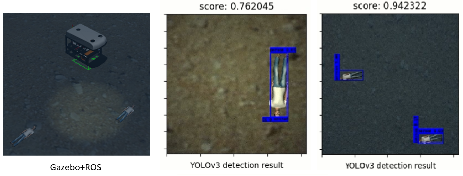
In this section, we illustrate EMTS using the Unmanned Underwater Vehicle Simulator [35], which is a ROS package designed for Gazebo robot simulation environment. We integrate it with YOLOv [29] for image classification and Concorde solver [32] to compute TSP tours. We use fidelity levels situated at m and m from the water floor, respectively. Fig. 2 shows our simulation setup, where victims are located at different locations on a water floor. At each sampling point, the vehicle take images and YOLOv returns an average score about the confidence level of the existence of victims in the view.
Each subplots of Fig. 3 shows the classification of regions before each epoch, the sampling points selected by the greedy policy and the planned path. Classifications of the environment are represented by colors: red means target exist, blue means no target, and green means uncertain. The dark green points and lines are the planned sampling locations and paths at the low fidelity level and red points and lines are sampling locations and paths at the high fidelity level. At the beginning of epoch , all regions are classified as uncertain. After first, second and third exploration tours, classified regions increases to , and , respectively. The detection task is terminated since more than of the regions are classified. Notice that the vehicle switches to the high fidelity level at epoch . The tours at low and high fidelity levels are plotted using two different colors. The vehicles do not sample in blue regions since they have been classified as empty. In the final result, the regions with target are successfully found. A video of the simulation is available as supplementary material.


In Fig. 4(a), we show the heat map of posterior variance for the whole region. The regions classified as empty have larger posterior variance since they have been eliminated from sampling space. This shows that EMTS is able to put more focus on areas likely to contain victims. The uncertainty reductions, i.e. the decreases of maximum posterior variance, by doing multi-fidelity greedy sampling and single-fidelity greedy sampling, are compared in Fig. 4(b). It shows that greedy multi-fidelity sampling can reduce uncertainty much faster at the beginning stage, which will enable EMTS to eliminate unoccupied regions quickly, and hence, accelerate target search.


V Analysis of EMTS
In this section, we analyze the modules of the EMTS algorithm and use these analyses to derive an upper bound on the expected detection time for the overall algorithm.
V-A Analysis of the classification algorithm
We first characterize the Bayesian confidence interval for , and then use this result to establish that the EMTS algorithm ensures a desired classification accuracy.
Lemma 1 (Bayesian confidence interval)
For and ,
Proof:
To normalize , let and Now , and from tail-inequality for standard normal distribution [36]
which prove the . Similar result holds for lower confidence bound. ∎
Theorem 2 (Misclassification Rate)
For the classification strategy in the EMTS algorithm, a location is misclassified with probability at most equal to .
Proof:
Consider a location such that , i.e., the true classification of is empty. Since at the end of epoch , the lower and upper confidence bounds used for classification employ , we apply a union bound to show the probability of classifying as a target satisfies
Then, it follows from Lemma 1 that the misclassification probability is no greater than . The case of location being occupied by a target follows similarly. ∎
V-B Analysis of the Sampling and Fidelity Planner
We now analyze the information gain and uncertainty reduction properties for our sampling and fidelity planner. We first recall some results for the single fidelity planner and then extend them to the case of multi-fidelity planner.
Consider a single-fidelity GP that is sampled with additive Gaussian noise with variance . Let be the set of first sampling points and let the vector of associated observations be . It is shown in [23, Lemma 5.3] that the mutual information between and is
| (7) |
where is the vector of calculated at points in . Let the maximal mutual information gain with samples be
Let be the total mutual information gain using a greedy policy that maximizes the summand in (7) at each sampling step. It follows, due to submodularity [37] of , that
While giving an exact value of is difficult, an upper bound on for squared exponential kernel derived in [23] is presented in the following Lemma 3.
Lemma 3 (Information gain for squared exp. kernel)
Let a GP be defined on domain . If has squared exponential kernel with length scale , then the maximum mutual information satisfies
Proof:
For a GP defined on with squared exponential kernel function , [23]. It is shown in [28] that scales with the area of . Thus, if the diameter of is , then . Note that having length scale in kernel function is equivalent to scale by . Accordingly, . For fixed , we omit diameter from the order notation and write . ∎
Lemma 3 provides a bound on the mutual information gain at the first fidelity level. For higher fidelity levels, the Gaussian process is composed of summation of independent GPs. We now establish that the information gained by sampling the sum of GPs is smaller than the information gained by sampling them independently, and then use this result to establish the bound on information gain for multi-fidelity GPs.
Lemma 4 (Information gain for sum of GPs)
Let and be independent GPs. Consider a measurement at point , where is additive measurement noise independent of and . Let be the vector of such measurements at sampling points in a set , where is the vector of i.i.d. measurement noise. Then,
Proof:
This result can established by applying the data processing inequality [38, Theorem 2.8.1]. ∎
Let be the maximal mutual information gain at fidelity . It follows from Lemma 4 and the multi-fidelity GP model in (2) that . Combining this inequality with Lemma 3, we obtain the following result.
Corollary 5 (Information gain for multi-fidelity GPs)
The maximal mutual information gain at fidelity satisfies
This corollary gives us an insight on the size of at different fidelity level. It follows that grows faster at higher fidelity levels.
We now derive a bound on the posterior variance for the multi-fidelity GP in terms of the maximum mutual information gain.
Lemma 6 (Uncertainty reduction for multi-fidelity GPs)
Let and , for each . An additive sampling noise is incurred every time is accessed. Under the greedy sampling policy the posterior variance after sampling rounds satisfies
Proof:
For any , is monotonically non-increasing in . So we get
| (8) |
where the second inequality is due to the fact . Again since , inequality (8) also indicates that is monotonically non-increasing. Hence, from (7), . Since is an increasing function on , σ_n-1^2(x_n) ≤ σ 2 log ( 1 + s -2 σ 2 ) log( 1 + s^-2σ_n-1^2(x_n) ). Substituting (8) into it, we conclude that
∎
Lemma 6 indicates that the smaller and the more slowly growing is, the faster converges. This result explains our idea of using multi-fidelity model.
V-C Analysis of Expected Detection Time
We now derive an upper bound on the number of samples needed to classify a location using EMTS algorithm and then use this result to compute the total sampling and travel time required for classification.
Lemma 7 (Sample complexity for uncertainty reduction)
In the autoregressive multi-fidelity model (3), if each has a squared exponential kernel, then
Proof:
It follows from Lemma 6 that
Since and for all fidelity levels are finite, it follows from Corollary 5 that . Combining these results, the lemma follows by inspection. ∎
Lemma 8 (Sample complexity for EMTS)
For a given misclassification tolerance , let be the number of samples required to classify . Then, the expected number of samples satisfies
where and .
Proof:
Since , function is monotonically decreasing for . We define
It can be shown that the choice of ensures, for ,
| (9) |
where and the second inequality is due to the fact . For a point at which and , based on (9), the number of sampling rounds to classify satisfies
where is the number of samples collected in the first epochs. Then the expected sampling rounds can be bounded as
From Lemma 7, we has . Therefore is finite. So we conclude
∎
Remark 1
(Comparison with sample complexity of multiarmed bandits:) Notice that describes the complexity to of classification of , i.e., for a point with close to th more time is needed. This term is similar to the sampling complexity [39] in a pure-exploration multi-armed bandit problem. This result is based on the assumption that GPs all have squared exponential kernel. For kernels characterizing less correlations, e.g. Martén kernels, more sampling rounds are expected.
We now derive an upper-bound on expected detection time for EMTS.
Theorem 9 (Expected classification time for EMTS)
For a location and misclassification tolerance , the expected classification time for satisfies
where .
Proof:
Since we assume unit sampling time, the total sampling time is in the same order as . Then we consider the traveling time spent in order to collected those samples. Since EMTS requires the vehicle to search from low fidelity level to high fidelity level, the total number of altitude switches is no greater than . As presented in [40], for points in , the length of the shortest TSP Tour . Therefore, the expected traveling time belongs to , where is the diameter of . Thus, the expected traveling time belongs to . Considering both sampling and traveling time, we conclude
∎Theorem 9 illustrates the efficiency of the EMTS algorithm, we conjecture it to be near optimal. It has a natural implication that the expected classification time at a location increases with the classification complexity and the desired classification accuracy.
VI Conclusions and Future Directions
In this paper, we extended the classical informative path planning approach for single-fidelity GPs to multi-fidelity GPs. This novel extension allowed for jointly planning for sampling locations and associated fidelity-levels, and thus, addresses the fidelity-coverage trade-off. We proposed and analyzed the EMTS algorithm for multi-target search that yields sampling points that the robot should visit and the fidelity level with which the robot should collect the information at these points. We illustrated our algorithm in an underwater victim search scenario using the Unmanned Underwater Vehicle Simulator. We rigorously analyzed the algorithm in terms of its accuracy in classifying the locations in the environment as empty or occupied by a target, as well as the expected time the robot takes to classify these points.
Future research include the extension to cooperative multi-robot search scenarios and implementation of the proposed algorithm in our underwater multi-target search testbed.
References
- [1] N. E. Leonard, D. A. Paley, F. Lekien, R. Sepulchre, D. M. Fratantoni, and R. E. Davis, “Collective motion, sensor networks, and ocean sampling,” Proceedings of the IEEE, vol. 95, no. 1, pp. 48–74, 2007.
- [2] S. L. Smith, M. Schwager, and D. Rus, “Persistent robotic tasks: Monitoring and sweeping in changing environments,” IEEE Transactions on Robotics, vol. 28, no. 2, pp. 410–426, 2012.
- [3] C. G. Cassandras, X. Lin, and X. Ding, “An optimal control approach to the multi-agent persistent monitoring problem,” IEEE Transactions on Automatic Control, vol. 58, no. 4, pp. 947–961, 2013.
- [4] R. N. Smith, M. Schwager, S. L. Smith, B. H. Jones, D. Rus, and G. S. Sukhatme, “Persistent ocean monitoring with underwater gliders: Adapting sampling resolution,” Journal of Field Robotics, vol. 28, no. 5, pp. 714–741, 2011.
- [5] A. Krause and C. E. Guestrin, “Near-optimal nonmyopic value of information in graphical models,” in Proceedings of the Twenty-First Conference Conference on Uncertainty in Artificial Intelligence, Edinburgh, Scotland, Jul. 2005, pp. 324–331.
- [6] C. K. Williams and C. E. Rasmussen, Gaussian processes for Machine Learning. MIT press Cambridge, MA, 2006, vol. 2, no. 3.
- [7] S. Vasudevan, F. Ramos, E. Nettleton, and H. Durrant-Whyte, “Gaussian process modeling of large-scale terrain,” Journal of Field Robotics, vol. 26, no. 10, pp. 812–840, 2009.
- [8] A. Singh, A. Krause, C. Guestrin, and W. J. Kaiser, “Efficient informative sensing using multiple robots,” Journal of Artificial Intelligence Research, vol. 34, no. 2, p. 707, 2009.
- [9] A. Krause, A. Singh, and C. Guestrin, “Near-optimal sensor placements in gaussian processes: Theory, efficient algorithms and empirical studies,” Journal of Machine Learning Research, vol. 9, no. Feb, pp. 235–284, 2008.
- [10] J. L. Ny and G. J. Pappas, “On trajectory optimization for active sensing in Gaussian process models,” in IEEE Conf on Decision and Control and Chinese Control Conference, Shanghai, China, Dec. 2009, pp. 6286–6292.
- [11] X. Lan and M. Schwager, “Planning periodic persistent monitoring trajectories for sensing robots in Gaussian random fields,” in IEEE Int Conf on Robotics and Automation, Karlsruhe, Germany, May 2013, pp. 2415–2420.
- [12] D. E. Soltero, M. Schwager, and D. Rus, “Generating informative paths for persistent sensing in unknown environments,” in IEEE/RSJ Int Conf on Intelligent Robots and Systems, Vilamoura, Algarve, Portugal, Oct. 2012, pp. 2172–2179.
- [13] J. Yu, M. Schwager, and D. Rus, “Correlated orienteering problem and its application to informative path planning for persistent monitoring tasks,” pp. 342–349, 2014.
- [14] V. Srivastava, F. Pasqualetti, and F. Bullo, “Stochastic surveillance strategies for spatial quickest detection,” The International Journal of Robotics Research, vol. 32, no. 12, pp. 1438–1458, 2013.
- [15] V. Srivastava, P. Reverdy, and N. E. Leonard, “Surveillance in an abruptly changing world via multiarmed bandits,” in IEEE Conference on Decision and Control, 2014, pp. 692–697.
- [16] G. A. Hollinger and G. S. Sukhatme, “Sampling-based robotic information gathering algorithms,” The International Journal of Robotics Research, vol. 33, no. 9, pp. 1271–1287, 2014.
- [17] G. A. Hollinger, B. Englot, F. S. Hover, U. Mitra, and G. S. Sukhatme, “Active planning for underwater inspection and the benefit of adaptivity,” The International Journal of Robotics Research, vol. 32, no. 1, pp. 3–18, 2013.
- [18] G. Hitz, E. Galceran, M.-È. Garneau, F. Pomerleau, and R. Siegwart, “Adaptive continuous-space informative path planning for online environmental monitoring,” Journal of Field Robotics, vol. 34, no. 8, pp. 1427–1449, 2017.
- [19] G. Hitz, A. Gotovos, M.-É. Garneau, C. Pradalier, A. Krause, R. Y. Siegwart et al., “Fully autonomous focused exploration for robotic environmental monitoring,” in 2014 IEEE International Conference on Robotics and Automation (ICRA). IEEE, 2014, pp. 2658–2664.
- [20] N. Atanasov, J. Le Ny, K. Daniilidis, and G. J. Pappas, “Information acquisition with sensing robots: Algorithms and error bounds,” in 2014 IEEE International Conference on Robotics and Automation (ICRA). IEEE, 2014, pp. 6447–6454.
- [21] A. A. Meera, M. Popović, A. Millane, and R. Siegwart, “Obstacle-aware adaptive informative path planning for uav-based target search,” in 2019 International Conference on Robotics and Automation (ICRA). IEEE, 2019, pp. 718–724.
- [22] Y. Sung, D. Dixit, and P. Tokekar, “Environmental hotspot identification in limited time with a uav equipped with a downward-facing camera,” arXiv preprint arXiv:1909.08483, 2019.
- [23] N. Srinivas, A. Krause, S. M. Kakade, and M. W. Seeger, “Information-theoretic regret bounds for gaussian process optimization in the bandit setting,” IEEE Transactions on Information Theory, vol. 58, no. 5, pp. 3250–3265, 2012.
- [24] P. Reverdy, V. Srivastava, and N. E. Leonard, “Modeling human decision making in generalized Gaussian multiarmed bandits,” Proceedings of the IEEE, vol. 102, no. 4, pp. 544–571, 2014.
- [25] S. Chen, T. Lin, I. King, M. R. Lyu, and W. Chen, “Combinatorial pure exploration of multi-armed bandits,” in Advances in Neural Information Processing Systems, 2014, pp. 379–387.
- [26] P. Reverdy, V. Srivastava, and N. E. Leonard, “Satisficing in multi-armed bandit problems,” IEEE Transactions on Automatic Control, vol. 62, no. 8, pp. 3788 – 3803, 2017.
- [27] M. C. Kennedy and A. O’Hagan, “Predicting the output from a complex computer code when fast approximations are available,” Biometrika, vol. 87, no. 1, pp. 1–13, 2000.
- [28] K. Kandasamy, G. Dasarathy, J. B. Oliva, J. Schneider, and B. Póczos, “Gaussian process bandit optimisation with multi-fidelity evaluations,” in Advances in Neural Information Processing Systems, 2016, pp. 992–1000.
- [29] J. Redmon and A. Farhadi, “Yolov3: An incremental improvement,” arXiv preprint arXiv:1804.02767, 2018.
- [30] P. Perdikaris, “Gaussian processes a hands-on tutorial,” 2017. [Online]. Available: https://github.com/paraklas/GPTutorial
- [31] S. Kemna, J. G. Rogers, C. Nieto-Granda, S. Young, and G. S. Sukhatme, “Multi-robot coordination through dynamic Voronoi partitioning for informative adaptive sampling in communication-constrained environments,” in 2017 IEEE International Conference on Robotics and Automation (ICRA). IEEE, 2017, pp. 2124–2130.
- [32] D. Applegate, R. Bixby, V. Chvatal, and W. Cook, “Concorde TSP solver,” 2006.
- [33] J.-Y. Audibert and S. Bubeck, “Best arm identification in multi-armed bandits,” in COLT, 2010, pp. 13–p.
- [34] E. Rolf, D. Fridovich-Keil, M. Simchowitz, B. Recht, and C. Tomlin, “A successive-elimination approach to adaptive robotic sensing,” ArXiv e-prints, 2018.
- [35] M. M. M. Manhães, S. A. Scherer, M. Voss, L. R. Douat, and T. Rauschenbach, “UUV simulator: A Gazebo-based package for underwater intervention and multi-robot simulation,” in OCEANS 2016 MTS/IEEE Monterey. IEEE, 2016, pp. 1–8.
- [36] M. Abramowitz and I. A. Stegun, Eds., Handbook of Mathematical Functions: with Formulas, Graphs, and Mathematical Tables. Dover Publications, 1964.
- [37] G. L. Nemhauser, L. A. Wolsey, and M. L. Fisher, “An analysis of approximations for maximizing submodular set functions,” Mathematical programming, vol. 14, no. 1, pp. 265–294, 1978.
- [38] T. M. Cover and J. A. Thomas, Elements of Information Theory. John Wiley & Sons, 2012.
- [39] S. Mannor and J. N. Tsitsiklis, “The sample complexity of exploration in the multi-armed bandit problem,” Journal of Machine Learning Research, vol. 5, no. Jun, pp. 623–648, 2004.
- [40] H. J. Karloff, “How long can a euclidean traveling salesman tour be?” SIAM Journal on Discrete Mathematics, vol. 2, no. 1, pp. 91–99, 1989.