Impact studies of nationwide measures COVID-19 anti-pandemic: compartmental model and machine learning
1. Introduction
The COVID-19 pandemic is testing the entire world so that measures are being taken in most nations to stem its development. These measures can generally be of different kinds such as social distancing, partial or total confinement, etc. It would therefore be interesting to be able to effectively analyze the effects of the measures taken on the spread of the pandemic. Here we offer an analysis of the impact of the measures taken that we apply to the case of Senegal. In previous papers [3], [11] and [12] we proposed a start of study using the results of [9].
In [9], a useful method for the study of the evolution of COVID-19 pandemic has been resented by using a compartmental model with Susceptible, Infected asymptomatic, Infected reported symptomatic and unreported symptomatic (SIRU). In [3], the author use that method to study the COVID-19 spread in Senegal with a classical SIR model.
In this work we aim to analyze the impact of the anti pandemic measures taken in Senegal. It is a continuation of the work done in [3]. We do a two-step analysis. The first uses the differential equations model denoted SIRU introduced in [9], and the second uses two machine learning tools: Predict of Wolfram Mathematica using Neural Networks method and Prophet.
We conduct the work in the following way. In the section 2 we study the effect of the nationwide measures by using an epidemic model presented in [9] and we present some machine learning tools. We show, in the section 3, the numerical results. In the section 4, we discuss the results. Then in section 5, we perform an analysis of the model and explain the parameters estimation. Finally in the section 6, we end by making a conclusion and advancing perspectives.
2. Analysis
2.1. Analysis of the measures
In [3] a classical SIR model was studied using results from the paper [9]. The aim was to analyze the effect of the nationwide measures using the data after nationwide measures. In fact, throughout to , we fitted an exponential function to the data of the total cases of infection of this period. represents the date of the nationwide measures, and is the starting time of the epidemic. We consider that the effects of the measures are such that they lead to a reduction in the contact rate. To describe this reduction, we chose a slowly decreasing function over time. We consider that the measures taken are not strong enough to systematically drop the contact rate to . This new function corresponds to the first one and the data in the period before measures from to , then takes a slower trajectory than that of the first function after . In other words, from the date , the new curve goes under the old one.
We consider that if on the dates the data goes under the new curve obtained with a contact rate after measures then, we can say that these measures affect the evolution of the pandemic.
In the previous paper [3], the function we fitted to the data from March to March by least square method, is with and (figure 1a). In this paper we fit a new exponential function to the data from March to April (figure 1b). For this new function, we have .


To continue in our analysis, we will use a differential equations model introduced in [9]. This model is as follows:
| (1) |
The initial conditions are , and and the initial time of the epidemic. With represents the susceptible individuals, the infected asymptomatic individuals, the unreported infected symptomatic and the reported infected symptomatic individuals.
We can also consider a version with removed compartments, the recovered and the death :
| (2) |
Let’s present the parameters. is the contact rate. is the average time during which asymptomatic infectious are asymptomatic. is the fraction of asymptomatic infectious individuals that become reported symptomatic infectious. is the average time symptomatic infectious have symptoms. is the rate at which asymptomatic infectious become reported symptomatic. is the rate at which asymptomatic infectious become symptomatic but unreported. is the proportion of recovered and is the proportion of death due to the infection.
We make the assumption that the function we fit the total number of reported infected cases is given by .
The starting time of the pandemic, the initial conditions and some parameters of the model are estimated and others are fixed. The parameters set are , and . The values chosen for and are those used by the medical authorities i.e. . Regarding the proportion of unreported and reported, we also use the same value proposed in [9], ie are reported and are unreported. Further detailed studies could make it possible to estimate the good value of this proportion for Senegal where we apply the model. For the estimation of the parameters, the starting time and the initial conditions, we use the calculation methods detailed in [9] and [3]. We start with the fitting exponential function which we equalize with the integral formula above . Hence some calculation of derivations, replacement in the model and integration gives:
- •
.
- •
, with .
- •
, with .
- •
, with .
- •
.
- •
.
- •
.
- •
.
For more details see section 5.
We consider that after the measures taken at the time , the contact rate depends on time following a formula we choose. We use two formulas. One of them was introduced in [3], and the second one was proposed in [10]. The first one is :
| (3) |
where and are parameters to choose. The second one is:
| (4) |
where is a parameter to choose.
Then the new model to solve is:
| (5) |
By solving (5), we get from which we can calculate the total number of infected with the formula . We choose values of parameters of such that follows the same path that . Then, by way of parameters and in , we can evaluate the measures. We do parametric solve with respect to parameters and . Results are shown in figure 5.
Now we consider at time , the nation applies stronger measures. We simply interpret as the contact rate is reduced by a factor . When the value of is equal to , it means that there are no measures, while when is equal to , it means that the strongest measures are taken. Hence the measures are quantified with the values of proportion . Then the contact rate become:
| (6) |
We solve the new model with replaced by . We do a parametric solve with respect to the parameter , and we plot the result for different values of . Then, we show different values of the peak, depending on the values of . Then, we can evaluate the maximal value of infection peak with respect to the level of the measures. Results are shown in figures 6, 7, 8 and 9.
2.2. Artificial Neural Networks
Artificial neural networks are part of artificial intelligence. Biological neural networks inspire them. Biological neural networks are part of the animal brain. One of the main functions of the brain is to process information, and the primary information processing element is the neuron. This specialized brain cell combines (usually) several inputs to generate a single output. Depending on the animal, an entire brain can contain anywhere from a handful of neurons to more than a hundred billion, wired together. The output of one cell feeding the input of another, to create a neural network capable of remarkable feats of calculation and decision making (See [13]).
If we could qualify the brain as a computer, then we would say that it is the best of computers. For this reason, the engineer seeks to improve mechanical computers to be closer to the biological computer, i.e., the brain.
The more neural connections there are, the more the network can solve complex problems. Pattern recognition is a task that neural networks can easily accomplish. For this task, introducing as input a pattern to a neural network, yields as output a pattern back (See [5]).
In general, neural network problems involve a dataset used to predict values for later datasets. For that, the neural network needs to be trained. Then, neural networks can predict the outcome of entirely new datasets based on training from old data sets.
Most neural network structures use some type of neuron, node, or unit. An algorithm called a neural network will generally be made up of individual interconnected neurons, see figure 3.
The artificial neuron receives input from one or more sources, which may be other neurons or data entered into the network from a computer program see figure 4. This entry is usually a floating-point or binary. Often the binary input is coded floating point representing true or false like or . Sometimes the program also describes the binary input as using a bipolar system with true as and false as .
An artificial neuron multiplies each of these inputs by a weight. It then adds these multiplications and transmits this sum to an activation function given by:
| (7) |
with the variables and represent the input and the weights of the neuron, is the number of input and weight.
Some neural networks do not use an activation function.
To read more about Neural Networks one can see [1], [5], [4] and [13].
Neural networks are implemented in machine learning tools of many software like Wolfram Mathematica[18]. We use the machine learning tool “Predict” to forecast the evolution of the COVID-19 pandemic in Senegal. We can choose different method of regression algorithm: “RandomForest”, “LinearRegression”, “NeuralNetwork”, “GaussianProcess”, “NearestNeighbors”, etc.
We use the “NeuralNetwork” regression algorithm, which predicts using artificial neural networks.
We consider two cases in the forecasting. The first case, only use the total number of infected case data in the training of the neural networks. While in the other forecasting, we use two types of data: the total number of infected cases and the contact rate. In the second case, the aim is to do forecasting by considering the effect of the contact rate. It is a way to show the effect of the nationwide measures taken at the time , as specified in section 2. For the contact rate we use as data given by (3).


2.3. Forecasting using Prophet
In this section, we develop another machine learning tool for forecasting to compare with the previous SIRU models and Neural Networks method.
We use Prophet [15], a procedure for forecasting time series data based on an additive model where non-linear trends are fit with yearly, weekly, and daily seasonality, plus holiday effects.
For the average method, the forecasts of all future values are equal to the average (or “mean”) of the historical
data. If we let the historical data be denoted by , then we can write the forecasts as
The notation is a short-hand for the estimate of based on the data . A prediction interval gives an interval within which we expect to lie with a specified probability. For example, assuming that the forecast errors are normally distributed, a 95% prediction interval for the -step forecast is
where is an estimate of the standard deviation of the -step forecast distribution.
For the data preparation, when we are forecasting at the country level, for small values, forecasts can become negative. To counter this, we round negative values to zero. Also, no tweaking of seasonality-related parameters and additional regressors are performed.
3. Numerical Simulations
3.1. Numerical analysis
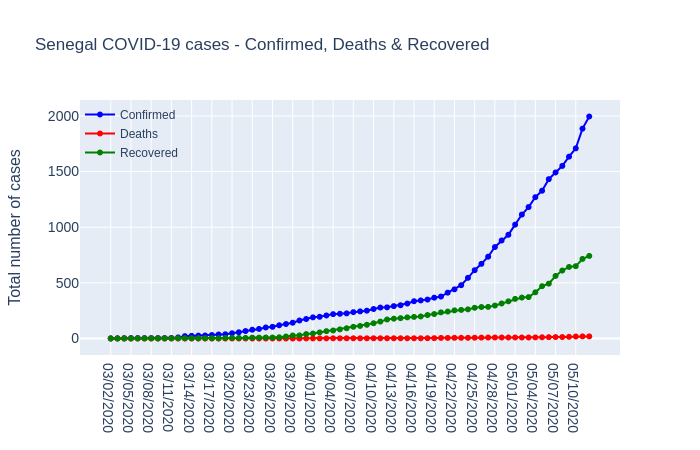
The data for Senegal, we use, is obtained from daily press releases on the COVID-19 from the Ministry of Health and Social Action (http://www.sante.gouv.sn/).
The figures 6, 7, 8 and 9 show results related to 2.1. The figures 6, 7 correspond to 3 and the figures 8, 9 correspond to 4.
We use the total population of Senegal is from
Senegal Population (2020) - Worldometer (www.worldometers.info). Then we obtain: , , , , .
The time of the nationwide measures in Senegal taken at 2020, March 23 is considered. Then . For given by (3), results are shown by figures 6a and 6b. For given by (4), results are shown by figures 8a and 8b. We see that the maximal number of reported case goes up to with the time peak at , which correspond to 2021, January 05.
A parametric plot of a parametric resolution of the SIRU model (5), using given by (3), with respect to and , is shown in figures 5.
Now, we consider that stronger measures is taken as explained in the subsection 2.1. The results is shown in figures 6c, 8c, 6d, 8d, 6e, 8e, 6f, 8f and 7.
Particularly figure 6c and figures 8c shows results of parametric solve of the SIRU model (5) with the parameters . Hence, we see that the time of the peak becomes , the date where stronger measures are taken. We choose as sample which correspond to 2020, May 10.
The figures 6d, 8d, 6e, 8e, 6f, 8f show parametric plot of the infected , the reported and unreported and total number of infected , with varying values of the parameter .
The figures 7 and 9 show again, in different range of the ordinate axis, parametric plot of the infected , the reported and unreported and total number of infected , with varying values of the parameter .


3.2. Comparative forecasting with machine learning
The forecasting is done with two data set. For both data from March 02, to April 25, 2020 and March 02, to May 12, 2020 we carry out simulations for a longer time and forecast the potential trends of the COVID-19 pandemic in Senegal. The predicted cumulative number of confirmed cases are first plotted for periods until May 26, June 10 and Sept. 18, 2020 ahead forecast with Prophet, with 95% prediction intervals.
The confirmed predictions for Senegal, using Prophet are given in Figure 12 (see Tables 2, 3 and 4 for the value of the confidence interval).
The figures 11 shows forecasting using Neural Networks method of Predict. Particularly the figure 11 shows two forecasting, one based only on data and an other obtained by training the Neural Networks method with data and contact rate. The prediction are done until 2020, May 26, June 10 and September 18.
| Until date | |||||
|---|---|---|---|---|---|
| 2020-05-26 | 1552.118087 | 1614.691394 | 1679.634752 | 1747.037931 | 1816.9941 |
| 2020-06-10 | 2785.471575 | 2894.759872 | 3008.187615 | 3125.911594 | 3248.094533 |
| 2020-09-18 | 118687.0026 | 123186.2236 | 127855.8589 | 132702.3632 | 137732.4357 |


| Date | |||
|---|---|---|---|
| 2020-05-22 | 2695.292384 | 2598.664351 | 2807.280554 |
| 2020-05-23 | 2777.228597 | 2663.535151 | 2897.959707 |
| 2020-05-24 | 2853.863973 | 2718.853527 | 2994.394743 |
| 2020-05-25 | 2945.018292 | 2802.374207 | 3095.868137 |
| 2020-05-26 | 3024.913096 | 2857.548751 | 3196.443359 |
| Date | ||||||
|---|---|---|---|---|---|---|
| 2020-05-22 | 2509.179622 | 2438.869281 | 2579.489963 | 2714.814079 | 2647.304599 | 2782.323560 |
| 2020-05-23 | 2575.632714 | 2505.322373 | 2645.943055 | 2803.067798 | 2735.558317 | 2870.577278 |
| 2020-05-24 | 2641.331365 | 2571.021025 | 2711.641706 | 2891.331968 | 2823.822488 | 2958.841449 |
| 2020-05-25 | 2706.266493 | 2635.956152 | 2776.576834 | 2979.590415 | 2912.080934 | 3047.099895 |
| 2020-05-26 | 2770.436355 | 2700.126014 | 2840.746696 | 3067.828454 | 3000.318974 | 3135.337935 |
| Date | |||
|---|---|---|---|
| 2020-06-06 | 3887.495614 | 3491.259628 | 4284.386057 |
| 2020-06-07 | 3964.130990 | 3541.984441 | 4387.085352 |
| 2020-06-08 | 4055.285309 | 3616.658728 | 4496.788853 |
| 2020-06-09 | 4135.180113 | 3685.960670 | 4604.522925 |
| 2020-06-10 | 4206.725884 | 3726.064523 | 4685.455882 |
| Date | ||||||
|---|---|---|---|---|---|---|
| 2020-06-06 | 3409.698565 | 3339.388223 | 3480.008905 | 4034.675309 | 3967.165829 | 4102.184790 |
| 2020-06-07 | 3462.752283 | 3392.441942 | 3533.062624 | 4122.100051 | 4054.590571 | 4189.609532 |
| 2020-06-08 | 3515.229377 | 3444.919036 | 3585.539718 | 4209.437690 | 4141.928209 | 4276.947171 |
| 2020-06-09 | 3567.143036 | 3496.832695 | 3637.453377 | 4296.685488 | 4229.176007 | 4364.194968 |
| 2020-06-10 | 3618.508442 | 3548.198100 | 3688.818782 | 4383.845435 | 4316.335955 | 4451.354916 |
| Date | |||
|---|---|---|---|
| 2020-09-14 | 11827.154428 | 7680.757057 | 15751.856303 |
| 2020-09-15 | 11907.049231 | 7721.053577 | 15888.511751 |
| 2020-09-16 | 11978.595002 | 7769.517365 | 15984.853526 |
| 2020-09-17 | 12051.967485 | 7776.250955 | 16102.077092 |
| 2020-09-18 | 12132.562027 | 7824.092604 | 16225.629593 |
| Date | ||||||
|---|---|---|---|---|---|---|
| 2020-09-14 | 7404.458859 | 7334.148519 | 7474.769201 | 12499.239975 | 12431.730495 | 12566.749456 |
| 2020-09-15 | 7439.797975 | 7369.487634 | 7510.108316 | 12582.463095 | 12514.953615 | 12649.972576 |
| 2020-09-16 | 7475.119671 | 7404.809330 | 7545.430012 | 12665.674270 | 12598.164790 | 12733.183751 |
| 2020-09-17 | 7510.423945 | 7440.113604 | 7580.734286 | 12748.868522 | 12681.359041 | 12816.378002 |
| 2020-09-18 | 7545.708310 | 7475.397969 | 7616.018651 | 12832.053814 | 12764.544334 | 12899.563295 |


4. Discussion
Analysis of the new trend in the data from March 2 to April 24, 2020 shows a change in the trajectory of the total number of cases. That causes a reduction of the maximum value of the peak compared to what it would have been without the measures taken on March 23, 2020. See figures 6a, 6b, 8b, 8a.
By considering new nationwide measures of Senegal, which we have chosen in this study to fix on the date of May 10, 2020, we note that the maximum value of the peak decreases according to the force of the measures taken. Likewise, the time of the peak is postponed as shown by the parametric plots in figures 6, 7, 8 and 9.
Since the first measures on March 23, 2020, Senegal has laughed at additional measures such as the closing of markets, shops, stores and other public places, with an opening calendar. We have therefore chosen May 10, 2020 as a date from which the additional measures can begin to take effect in reducing contamination.
We see that depending on the strength of these measures, the evolution of the disease can lose its exponential nature or become slower.
The prediction with neural networks and Prophet show an optimistic situation. The forecasting based only on data and those on contact rates show a slow evolution as shown in figures 11 and 12.
We see that the curve obtained using the contact rate function in training of the neural networks, goes below that obtained only using the data on the total number of cases.
5. Materials and methods
5.1. Basic proprieties
Let’s set , is the initial population. Replacing an initial solution in the system (1), we obtain:
| (8) |
Solving these differential inequalities gives , and . Hence .
By considering an initial solution with , we get . Then .
Now, summing the equations of the system (1), we obtain .
Then . Finally remain in the set .
This implies that is a positively-invariant set under the flow described by (1). In addition, the model can be considered as being epidemiologically and mathematically well-posed.
Let’s set
| (9) |
Then the system (1) with initial condition can be rewritten in the following form:
| (10) |
Theorem 5.1.
The system (10) has a unique solution for .
Remark 5.1.
The proof of the above theorem come from the Cauchy-Lipschitz theorem and the Fundamental Existence-Uniqueness theorem in [14], since .
Theorem 5.2.
Proof of Theorem 5.2.
The proof of the existence uniqueness of the system (11) with (3) and (4) are similar. Then, we do this for one.
The function is piece-wise continuously differentiable in . Then by using the theorem 5.1, we have the existence of a unique solution on of the system
and for the parameters and fixed, there is a unique solution for of the system
.
Now defining the function , we deduce that is a unique solution continuous in time of the system (11).
∎
5.2. Disease Free Equilibrium
The unique equilibrium of the model (1) is the canonical DFE given by .
5.3. Parameters estimation
The estimation of the parameters of the model (1) is done by using techniques in [9], [3]. We fit the cumulative data with an exponential function . In addition, we assume that the cumulative function can be given in integral form as .
Then . Thus, we obtain .
Also we have:
| (12) |
Then and . Hence, we obtain
| (13) |
then and .
Let’s set and such that and .
Then replacing in the second an third equation of the following system:
| (14) |
we obtain
| (15) | ||||
| (16) |
Then introducing (16) in the first equation of (14), we obtain:
Hence
| (17) |
Replacing (16) in (17), we obtain:
| (18) |
5.4. The basic reproductive number
6. Conclusion and perspectives
In this paper, we have analyzed the impact of anti-pandemic measures in Senegal. First, we used techniques of fitting function to the data of the total number of cases. The choice of the data fit function is crucial for the results since it allows the estimation of the parameters of the compartmental model used. In a second work, we use machine learning tools to also predict the future evolution of the pandemic in Senegal. Also, we have integrated the effects of the measures into the prediction.
Depending on the measures taken, the pandemic’s trajectory may become slower or lose its exponential nature.
It would be interesting, in the following, to use other functions of a slow nature like the logistical function to fit data and thus obtain different results. A stochastic study using Brownian motions applied to the SIRU compartmental model would also be interesting.
Acknowledgement
The authors thanks the Non Linear Analysis, Geometry and Applications (NLAGA) Project for supporting this work.
Conflict of interest
The author declares no conflict of interest.
References
- [1] Alpaydin, E. (2010) Introduction to Machine Learning 2nd ed, 584. Adaptive Computation and Machine Learning.
- [2] Anderson, R. M. and May, R. M. (1992) Infectious Diseases of Humans, 768. Oxford University Press, Oxford.
- [3] Baldé, M.A.M.T. (2020) Fitting SIR model to COVID-19 pandemic data and comparative forecasting with machine learning, medRxiv preprint doi: https://doi.org/10.1101/2020.04.26.20081042.
- [4] Goodfellow, I., Bengio Y. and Courville, A. (2016) Deep Learning, MIT Press. http://www.deeplearningbook.org
- [5] Heaton, J. (2015) AIFH Volume 3: Deep Learning and Neural Networks, Heaton Research, Inc, 268. Tracy Heaton (2015).
- [6] Hethcote, H. W. (2000) The Mathematics of Infectious Diseases, Society for Industrial and Applied Mathematics, Vol. 42, No. 4, pp. 599–653.
- [7] Langtangen, H. P. and Pedersen, G. K. (2016) Scaling of Differential Equations, 152. Springer.
- [8] Di Lauro, F. , Kissy, I.Z. and Miller, J.C. (2020) The timing of one-shot interventions for epidemic control, medRxiv preprint doi:https://doi.org/10.1101/2020.03.02.20030007.
- [9] Liu, Z., Magal, P., Seydi, O., and Webb, G. (2020) Understanding Unreported Cases in the 2019-Ncov Epidemic Outbreak in Wuhan, China, and the Importance of Major Public Health Interventions, SSRN: https://ssrn.com/abstract=3530969 or http://dx.doi.org/10.2139/ssrn.3530969.
- [10] Liu, Z., Magal, P., Seydi, O., and Webb, G. (2020) Predicting the cumulative number of cases for the COVID-19 epidemic in China from early data, medRxiv preprint https://doi.org/10.1101/2020.03.11.20034314.
- [11] Ndiaye, B.M., Tendeng, L. and Seck, D. (2020) Analysis of the COVID-19 pandemic by SIR model and machine learning technics for forecasting. https://arxiv.org/abs/2004.01574v1.
- [12] Ndiaye, B.M., Tendeng, L. and Seck, D. (2020) Comparative prediction of confirmed cases with COVID-19 pandemic by machine learning, deterministic and stochastic SIR models. https://arxiv.org/abs/2004.13489.
- [13] Newman, M. E. J. (2010) Networks An Introduction, Oxford University Press, 394.
- [14] Perko, L. (1991) Differential equations and dynamical systems, Springer-Verlag New-York.
- [15] Prophet: Automatic Forecasting Procedure, avalailable in https://facebook.github.io/prophet/docs/ or https://github.com/facebook/prophet.
- [16] Python Software Foundation. Python Language Reference, version 2.7. Available at http://www.python.org.
- [17] Van den Driessche, P. and Watmough, J. (2002) Reproduction numbers and subthreshold endemic equilibria for compartmental models of disease transmission, Mathematical Biosciences 180, 29-48.
- [18] Wolfram Mathematica, https://www.wolfram.com/mathematica/?source=nav.