Floquet theory for temporal correlations and spectra in time-periodic
open quantum systems: Application to squeezed parametric oscillation
beyond the rotating-wave approximation
Abstract
Open quantum systems can display periodic dynamics at the classical level either due to external periodic modulations or to self-pulsing phenomena typically following a Hopf bifurcation. In both cases, the quantum fluctuations around classical solutions do not reach a quantum-statistical stationary state, which prevents adopting the simple and reliable methods used for stationary quantum systems. Here we put forward a general and efficient method to compute two-time correlations and corresponding spectral densities of time-periodic open quantum systems within the usual linearized (Gaussian) approximation for their dynamics. Using Floquet theory we show how the quantum Langevin equations for the fluctuations can be efficiently integrated by partitioning the time domain into one-period duration intervals, and relating the properties of each period to the first one. Spectral densities, like squeezing spectra, are computed similarly, now in a two-dimensional temporal domain that is treated as a chessboard with one-period one-period cells. This technique avoids cumulative numerical errors as well as efficiently saves computational time. As an illustration of the method, we analyze the quantum fluctuations of a damped parametrically-driven oscillator (degenerate parametric oscillator) below threshold and far away from rotating-wave approximation conditions, which is a relevant scenario for modern low-frequency quantum oscillators. Our method reveals that the squeezing properties of such devices are quite robust against the amplitude of the modulation or the low quality of the oscillator, although optimal squeezing can appear for parameters that are far from the ones predicted within the rotating-wave approximation.
I Introduction
In recent years, with the development of new quantum technologies, more complex protocols to control and manipulate quantum devices have been proposed. Usually, those devices are made up of nearly isolated quantum systems (atoms, solid-state defects, superconducting circuits, mechanical elements, etc) that interact coherently with the electromagnetic field (at optical or microwave frequencies) via an input port, where a driving is applied, and an output port, where the detection is performed. Also, the considered quantum system can interact with its environment, usually leading to an incoherent exchange of excitations which manifests as noise (thermal, electronic, etc). A proper engineering of all these processes is key to design quantum technologies for applications in quantum computation, simulation, communication, and metrology.
In the context of cavity quantum optics (where we also consider the related fields of superconducting-circuit resonators, polariton microcavites, and cavity optomechanics), as well as in the field of many-body physics, several works based on periodically-modulated driving have appeared recently in the literature aimed at controlling or enhancing specific features, as well as promoting the emergence of new phenomena and even novel phases of matter. The use of modulations has been proposed, for instance, for generating two-mode entangled states in superconducting circuit resonators (QubitEntangled), quantum squeezing of the mirror motion (MechSqueezingTh; MechSqueezing; Mari; Farace) or of the radiation field in optomechanical (LightSqueezing; Garces2016; Levitan) and superconducting-circuit cavities (Garces2016), for producing entanglement between a mechanical and an optical mode or between two radiation modes (Farace; Mari-NJP; Liao), for entangling the motional degrees of freedom of two tethered and optically-trapped microdisks inside a cavity (Abdi), for cooling the ground state of a mechanical oscillator (rocking-Zhang), for measuring the position of a mechanical oscillator in an optomechanical backaction-evading scheme (Evasion; Evasion1), for enhancing nonlinear interactions in quantum optomechanics (Lemond), or for synchronization or entrainment purposes (sync1; sync2; sync3; sync4; sync5; sync6; sync7; sync8; sync9; sync10) with its implications in the emergence of quantum correlations and entanglement (Zambrini; Timme). Such periodic or multi-periodic drivings can also be used to engineer elusive dissipative models such as squeezed lasers (CNB-SqueezedLasing), degenerate parametric oscillation (CNB-DPO-OM; Legtas15), and non-reciprocal devices (Anja2; Anja3; Anja4; Anja5) with a range of applications (AnjaApp1; AnjaApp2; Anja1). Moreover, spontaneous periodic oscillations (also called limit cycles) can emerge in nonlinear systems, usually via Hopf bifurcations. In particular, such oscillations have been observed experimentally in optomechanical cavities operating in the classical regime (HBexp1; HBexp2; HBexp3; HBexp4), and are well understood theoretically (HBth1; HBth2; HBth3). In contrast, the study of quantum dynamics around limit cycles is a very active field of theoretical research in different contexts (HBq1; HBq2; HBq4; HBq5; HBq6; LC; LC-Hartmann; LC-JJ; RefA1; RefA2; RefA3), including their connection to the emergence of time crystals (Frank12quantum; Frank12classical; Frank19; TCreview) in driven-dissipative many-body systems (OpenTC1; OpenTC2; OpenTC3; OpenTC4; OpenTC5; OpenTC5bis; OpenTC6; OpenTC7). Closely related to the latter is the field of Floquet or discrete time crystals in periodically-driven closed many-body systems (DTC1; DTC2; DTC3; TCreview; DTCapps1), which have only recently been identified as unconventional phases of matter far from equilibrium (DTC4; DTC5; DTC6; DTC7; DTC8), but have already sparked interesting experiments (DTCexp1; DTCexp2; DTCexp3; DTCexp4; DTCexp5; DTCexp6; DTCexp7; DTCexp8) and applications (DTCapps1; DTCapps2). Also in this context, periodic modulations allow for the so-called Floquet engineering of Hamiltonians (Shirley), leading to some desired properties such as nontrivial topology or optimized transport (Hanggi98; FloquetEngineering).
Taking all these things into consideration, it is clear that periodic modulations play a major role in many different fields of contemporary quantum physics. In this work, we will concentrate on periodically-driven open quantum-optical systems. There are two standard mathematical descriptions of such quantum systems: (i) via a set of coupled quantum Langevin equations, which are Heisenberg (differential) equations for the operators supplemented by dissipation terms and input quantum noises, or (ii) via a master equation for the density operator, which consists on the von Neumann equation for the state, to which Lindblad terms accounting for irreversible quantum jumps are added. Let us remark that master equations can be mapped to a set of stochastic Langevin equations by resorting to phase-space representations of the density operator (like the Wigner function or, more robustly, the positive P distribution (PositiveP1; PositiveP2; PositiveP3)). Hence, in both approaches a set of Langevin equations can be ultimately obtained, which provide a route towards the numerical analysis of dynamical features.
Due to the generally nonlinear nature of such equations, exact solutions are hard or impossible to find, except for very specific cases. Analytic or semi-analytic insight is usually gained by using the so-called standard linearization technique, which typically provides sensible results, except close to phase transitions or in the presence of spontaneous symmetry breaking, which nevertheless can be treated with suitable generalizations of such technique (CNB08; CNB09; CNB10; CNB-PhD; CNB14-Linear; CNB15-Linear; SPOPOrot; LC). Within this approach, one considers small quantum fluctuations around a reference classical state, leading to a linear system of Langevin equations for the fluctuations, which is easily handled only if the classical reference is time independent. This can occur in problems involving a constant pump, like the laser, or even in the presence of a monochromatic drive, as in optical parametric oscillators (CNB-PhD) and optomechanical cavities (OM) (but only if a rotating-wave approximation can be invoked). However, even in such cases, the stationary classical solutions can become unstable (e.g. via a Hopf bifurcation), and spontaneous oscillations can emerge in the classical dynamics, leading to nontrivial linearized Langevin equations for the fluctuations, which in particular will contain now time-periodic coefficients that make them hard to treat. The same happens if the drive contains more than one frequency (or if the rotating-wave approximation cannot be used), in which case it is in general impossible to obtain time-independent classical states.
For this type of linear Langevin equations with time-periodic coefficients, common strategies are based on Fourier expansions (Mari; FloquetApproach; FourierApproach). Recently, however, we put forward a more compact approach based on the Floquet theorem (LC), which transforms linear homogeneous differential equations with periodic coefficients into equivalent equations with constant coefficients. There, however, we focused on the determination of the asymptotic covariance matrix for long times, and its connection with the steady state of the master equation after diffusion around the limit cycle has taken over. In this work we go deeper into the general Floquet method for linearized systems, in particular using it to develop an efficient method for the computation of experimentally-relevant quantities such as two-time correlation functions and the corresponding spectral densities. Specifically, we show how these quantities can be evaluated just from knowledge of the behavior of the system during a single period, which is crucial in order to avoid significant errors in the computation of such observables: a large numerical effort can be employed at a low cost to perform highly precise integrations along one period, and then propagate that information algebraically over the long term.
As a practical example, we use the theory to analyze the squeezing properties of degenerate parametric oscillators beyond the rotating-wave approximation, which has become a timely issue, since such a model can be implemented nowadays in low-frequency superconducting oscillators well within the quantum regime (Legtas15). Our results support the robustness of squeezing against the modulation amplitude or the bad quality of the oscillator. Moreover, we show that once counter-rotating terms are incorporated, optimal squeezing is achieved for modulation amplitudes below the oscillation instability, contrary to the rotating-wave predictions, for which optimal squeezing always occurs at the instability.
The manuscript is organized as follows. In Sec. II we briefly review the description of open quantum systems via linearized Langevin equations, and introduce the Floquet-based method for the determination of their solutions. In Secs. III-V we use the solutions to manipulate two-time correlations and the corresponding spectral densities, producing compact expressions solely based on dynamics over a single period. Finally, in Sec. VI we apply the theory to degenerate parametric oscillation beyond the rotating-wave approximation.
II Linearization in time-periodic open quantum systems: Floquet theory
Consider an open quantum system furnished with a set of operators , where the symbol denotes transposition. The system evolves according to its own dynamics as well as to interactions with its environment, which in general is composed of several reservoirs with which the system exchanges energy. In the Heisenberg picture, which we adopt, and assuming standard Markovian conditions, the system operators evolve generically according to some quantum Langevin equations
| (1) |
Here accounts for the deterministic, Hamiltonian or not, part of the dynamics and depends on the system operators and also on a set of control parameters generically denoted by (e.g. the amplitude and frequency of a driving field). These can be time dependent thereby inducing periodic dynamics in the classical limit. The fluctuations fed by the reservoirs into the system, responsible for irreversible quantum jumps, enter the dynamics through a noise term. With full generality, we write it as a matrix (that might depend as well on the control parameters and the system operators) acting on a vector composed of Gaussian white noises with and two-time correlators , which define a noise-correlation matrix . Note that the number of independent noises needs not equal (e.g. in an optical cavity there are several input vacua per mode, even if in many instances one can ignore all but one).
Let us remark that the stochastic Langevin equations naturally obtained from the Schrödinger picture through phase-space representations such as the positive (PositiveP1; PositiveP2) have the same form as Eq. (1), but replacing operators by suitable stochastic variables. Hence, the theory that we are going to put forward applies also to such an alternative, but common approach to open quantum systems.
Note that throughout this work we use bold fonts for vectors, e.g. , which by default correspond to columns with components denoted by , so that corresponds to a row vector; also, a dagger will denote the conjugate-transpose as usual, e.g. . On the other hand, we use calligraphic fonts for matrices, e.g. , whose components we denote by .
We follow the standard linearization procedure that starts by splitting each operator as its mean field plus a fluctuation , i.e. . In the semiclassical approximation that is commonly adopted, the mean field , to be denoted as , is ruled by the dynamical system of equations , obtained from Eq. (1) by substituting operators by their mean values and ignoring noises. These correspond to the classical limit, and we are here interested in the case where such classical dynamics is periodic, i.e. , with some periodic function with period . This can happen either when the control parameter is periodically modulated in time, or following a dynamical (typically Hopf) bifurcation occurring at some critical value which marks the onset of self-sustained oscillations (see (LC) for a detailed example).
The dynamics of the fluctuations is governed by the original quantum Langevin equations (1), which after linearization with respect to fluctuations and noises are written as
| (2) |
where we denote simply by , and the -matrix is the Jacobian of the classical dynamical equations, with elements . The Jacobian depends on the parameters and on the classical solution, and thus it is explicitly -periodic, , as is the matrix . Hence (2) is a non-autonomous dynamical system of linear equations, which prevents its analytical solving. However application of Floquet theory allows us to transform Eq. (2) into a system with a time-independent Jacobian, which is more amenable to analytical or semi-analytical treatments. Let us review here the procedure, which we will exploit throughout the rest of the work RefAFloquet1; RefAFloquet2; RefFloquet3; RefFloquet4. We start by defining the principal fundamental matrix through the initial-value problem
| (3) |
where is the identity matrix. Note that we choose the initial time as 0 without loss of generality, because any other choice, e.g. with , is connected to Eqs. (2) and (3) by the change of variables and , leading to a Floquet problem with associated principal fundamental matrix . Next, we construct a constant matrix through
| (4) |
which serves to decompose the fundamental matrix in its so-called Floquet normal form,
| (5) |
where is a -periodic invertible matrix. Defining a transformed fluctuation vector
| (6) |
the non-autonomous equation (2) with time-periodic coefficients turns into
| (7) |
which is an equation with time-independent coefficients and time-dependent forcing. This constitutes an example of Floquet’s theorem.
The system of equations (7) can be formally solved in terms of the eigensystem of matrix . Let us denote by the matrix that diagonalizes through the similarity transformation
| (8) |
The eigenvalues are known as Floquet (or characteristic) exponents. Note that in previous works (LC) we have used a slightly less compact notation, where we defined the set of right and left eigenvectors of , satisfying , , and orthonormality relations . These two notations are connected by
| (9) |
It proves convenient to define the auxiliary matrix
| (10) |
Upon multiplying (7) by from the left, and defining the projections
| (11a) | ||||
| (11b) | ||||
we get
| (12) |
which are a set of decoupled linear equations for the components of , whose formal solution can be put as
| (13) |
Here we assumed that all the eigenvalues have negative real part (i.e., the analyzed semiclassical state is linearly stable), hence the integral (13) is bounded.
Expressions (3), (4), (5), (8), and (13) constitute the basis of our analysis, as they allow computing the fluctuation vector
| (14) |
in terms of the noise integrals that depend only on the auxiliary matrix and the Floquet exponents .
Note that computing matrix is not required at any step. Instead, we can use the so-called monodromy matrix , which is diagonalized by the same similarity transformation (8), and possesses eigenvalues related to the Floquet exponents by .
III Computation of two-time correlations
Our goal is the computation of physical quantities related to the quantum fluctuations of the system around the stable, periodic semiclassical solution . Within the linearized approximation that we are using, which is equivalent to assuming the state to be Gaussian CNB14-Linear; CNBbook, the most general quantities that one can consider are two-time correlations, since for Gaussian distributions any higher-order correlation can be reduced to products of two-time ones. Hence, the most general correlators we want to compute are
| (15) |
where we remind that is a column vector, so is a matrix. As a first result of this work, we provide here a simple expression for this two-time correlation matrix that exploits the periodic nature of the problem. We start by using (14) to rewrite it as
| (16) |
where
| (17) |
are elementary correlations that we work out in Appendix A. We relegate the technical derivations to that appendix, and summarize here only the final compact expressions. Note first that the projected noises (11b) are delta correlated as
| (18) |
with a projected-noise correlation matrix that is obviously -periodic. With this definition at hand, we show in Appendix A that the correlation matrix (17) can be worked out to yield the components
| (19) |
where
| (20a) | ||||
| (20b) | ||||
with
| (21a) | ||||
| (21b) | ||||
Eqs. (19)-(21) are the first main result of this work as they allow us to compute any two-time correlation in terms of integrals of functions evaluated just in the interval . The importance of this result emerges when long measurement times are involved, as those required for the computation of spectral densities (see next section), because, apart from being numerically demanding, the errors accumulated in finding the fundamental matrix at long times can be large enough to invalidate the results.
Note that, for numerical purposes, it is typically more efficient to evaluate from the equivalent initial-value problem
| (22) |
rather than from the integral (21b).
IV Computation of spectral densities
Another important tool for characterizing quantum fluctuations are the spectral densities associated to two-time correlations. A relevant example is the light squeezing spectrum, which is the spectral variance of the (quantum) noise carried by a light beam, and can be measured experimentally via balanced homodyne detection (Gea; CNB-PhD) or alternative correlation measurements (Vogel). In the usual stationary case, i.e. when two-time correlations are a function only of the two-time difference, these densities are just plain Fourier transforms. However, when such correlations are not stationary one has to use a different definition in order to match the experimentally detected spectral density (Gea; CNB-PhD), namely
| (23) |
where is the considered two-time correlation and is the detection time. In general the measurable densities will be linear combinations of and , as we will see later through a practical example. We then consider spectral densities of the form
| (24) | ||||
obtained upon setting in (23), being and generic -periodic functions whose meaning is as follows. When such functions are chosen as and , respectively, and summing over and , one can compute spectral densities corresponding to the correlations , see (16). The choice is also interesting as it provides the spectral densities corresponding to the elementary correlations , which in some cases are proportional to measurable quadratures (CNB-PhD; CNB08; CNB09; CNB10; SPOPOrot). Finally, when is formed of annihilation and creation operators, with the choice and , (24) allows the computation of spectral densities corresponding to homodyne-detection experiments when the local oscillator is a -periodic function SPOPO, in which case and are proportional to the amplitude (or its complex conjugate) of that local oscillator.
At first sight it seems easy to solve the problem once the correlation functions have been expressed in Eqs. (19) in terms of the first period. However, for long measurement times, as realistically needed, the integrals are still numerically demanding and can carry important numerical errors. In order to avoid this, we have worked out Eq. (24) by exploiting the properties of the integral’s kernel, and managed to simplify it into a few integrals defined only over a single period. As we did in the previous section, we relegate the technical derivations to Appendix B, presenting here the final result. Moreover, we focus on the common situation of a long detection time that contains very many periods, that is, . In this limit, as proven in Appendix B, the general spectral density (24) is simplified as
| (25) | ||||
where
| (26a) | ||||
| (26b) | ||||
| (26c) | ||||
| (26d) | ||||
Let us remark that the superindex labeling each integral is not arbitrary, but connected to the original integration domain from where they emerge in the space. In particular, in Appendix B we show that dividing the space into a sort of chessboard with squared integration domains of area , is the integral to which we can relate all the integrals defined on squares below the diagonal, hence the ‘’ label.
Remarkably, again we have been able to write spectral densities in terms of first-period objects only, which comes with all the numerical benefits that we highlighted above. Hence, this is the second main result of our work, which provides a compact way of evaluating arbitrary spectral densities in periodic systems from knowledge of the Floquet eigensystem over a single period.
Similarly to what we did in the previous section with in Eq. (22), it is useful for numerical efficiency to find the integrals defined above from their equivalent differential equations. In the case of and , both are of the integral form . Hence, defining two independent initial-value problems
| (27a) | ||||
| (27b) | ||||
we get . On the other hand, and are of the nested type , which makes their differential form a bit more intricate, but equally efficient from a numerical standpoint. In this case, we first solve the initial-value problem
| (28) |
backwards in time in the domain , and next the initial-value problem
| (29) |
so that .
V Cross-correlations and cross-spectra with the noise
In the previous sections we focused on the two-time correlations and spectral densities of the variables (or, equivalently, the projections ). However, in many situations one also needs objects related to the cross-correlations between the variables and the noises . A most prominent case is related to the evaluation of quantities related to the field leaking out of the open system by using input-output relations. We will showcase this in the practical example that we consider in the next section. This section is then devoted to provide compact expressions for these type of cross-correlations and spectral densities. Again we make all technical derivations in Appendix C, and offer here just the final results.
We start by providing the two-time cross-correlators between the projections and the noises , which are easily worked out as
| (30a) | |||
| and | |||
| (30b) | |||
where we have defined the matrices and . Let us remind that is the auxiliary matrix defined in Eq. (10), is the matrix multiplying the noise vector in the linearized equations (2), and is the matrix defined after Eq. (1) summarizes the two-time correlators of the noise as .
VI Application: Degenerate parametric oscillation beyond the rotating-wave approximation
As an application of the method developed above, we consider now the degenerate parametric oscillator as an example. In essence, it consists of a lossy quantum-mechanical harmonic oscillator whose frequency is modulated periodically at twice its natural frequency (parametrically-driven oscillator). This model serves as the canonical one for the study of quantum squeezing, and has been traditionally explored experimentally with nonlinear optical cavities CNB-PhD. Since in this context accessible modulation amplitudes are much smaller than optical frequencies, one can perform a rotating-wave approximation that maps the problem to an effective time-independent one. In contrast, modern implementations based on low-frequency oscillators (e.g., in superconducting circuits Legtas15 or optomechanical devices CNB-DPO-OM) allow to explore the regime where the modulation amplitudes are a significant fraction of the oscillation frequencies. Under such conditions, the predictions derived within the rotating-wave approximation require corrections, and it is our purpose to study these here.
VI.1 The model
Consider an oscillator of mass and intrinsic frequency , with position and momentum , such that . We can describe the modulated case by the Hamiltonian
| (33) |
with (normalized) modulation amplitude . Let us write the position and momentum in terms of annihilation and creation operators as
| (34) |
with . Let us consider the slowly-varying operator , where is the Heisenberg-picture operator. This operator evolves according to , with rotating-picture Hamiltonian
| (35) |
In the limit , one can invoke the rotating-wave approximation, which allows neglecting the rapidly-oscillating terms, leading to the time-independent Hamiltonian . This is the usual Hamiltonian employed to analyze degenerate parametric oscillators. Here, in contrast, we use the theory developed in the previous sections to study the full Hamiltonian (35).

In order to include losses, we consider the interaction between the oscillator and a bosonic environment at zero temperature. Assuming that the standard Born-Markov approximation holds (see below for further discussion on this point), one can integrate out the environment leading to the quantum Langevin equation
| (36) |
where we have defined the normalized modulation amplitude , and is the so-called input operator, which is Gaussian and characterized by the following statistical properties:
| (37) |
Let us also remark that the slowly-varying operator is actually the one that homodyne detection is sensitive to, so this is the one we will use to compute the relevant spectral densities, as explained below.
It is convenient to introduce the dimensionless time , which we adopt in the following but removing the tilde for notational simplicity. Let us further define the vectors and , from which we build the quadrature vectors and , with . In terms of quadratures, Eq. (36) is then written as the linear system
| (38) |
which has the form of a Floquet problem (2), with the identifications , , , and Jacobian with
This Jacobian has periodicity in terms of the normalized frequency , which coincides with the resonator quality factor.
Note that we have obtained a linear system of equations directly, because our initial Hamiltonian (33) was quadratic. This is however an idealization that works only in a limited range of parameters, whose breakdown is signaled by the equations becoming unstable. For example, within the common rotating-wave approximation valid when as mentioned above, and obtained from (38) by neglecting the oscillatory terms in (39), the Jacobian takes the diagonal form with eigenvalues . Hence, this idealized linear picture is valid only for . Beyond such point, the modulation cannot be treated as a given term anymore, and needs a dynamical treatment of its own, for example as a dynamical variable that feels some backaction from the oscillator (known as pump depletion in optical implementations). Similar behavior is to be expected beyond the rotating-wave approximation, but this time signaled by the real part of some Floquet exponent becoming positive.
Finally, let us comment on the validity of Eq. (36) as a model for the effect of the environment onto the oscillator. Technically, this simple quantum Langevin equation is bound to break down for sufficiently small and large , when Born-Markov conditions can no longer be ensured. More refined and complex open models can be derived in these limits Hanggi0; Hanggi1; Hanggi2, but in order to illustrate our Floquet-based method, we will stick with the simple model of Eq. (36), commenting on the effects that it predicts as we depart from the ideal and conditions traditionally considered in the literature.
VI.2 Spectral covariance matrix
In order to understand the squeezing properties of this system, we will consider the spectral covariance matrix, which is the standard object recovered via homodyne detection of the excitations that leak out of the oscillator (e.g., the light exiting the cavity through a partially transmissive mirror in a degenerate parametric oscillator). Introducing the output operator
| (40) |
the spectral covariance matrix is defined as
| (41) |
with
| (42) |
We remind that we are working with a dimensionless time, and therefore, the detection frequency in this equation is also dimensionless, with the real detection frequency given by . The spectral covariance matrix (41) is subject, for all , to the usual constrains of the standard covariance matrix of Gaussian states (CNBbook; Patera20). For example, it is real, symmetric, and must posses positive eigenvalues (corresponding to the spectral density of the normal quadratures of the problem), and it satisfies the condition linked to Heisenberg’s uncertainty relations.
Note that has the same form as the generic spectral density that we defined in (23), just replacing the generic correlation function by the output correlation matrix . Hence, we now proceed to rewrite it in terms of the spectral densities that we have defined in the previous sections. First, note that can be written in terms of the previously defined correlations (17) and (30) as
| (43) | ||||
where we have used (40), (14), and the two-time correlators of the noises as defined after Eq. (1). Using now the definitions for the spectral densities that we introduced in (24) and (31), the components of are rewritten as
| (44) | ||||
an expression that is readily evaluated using the results of the previous sections. Specifically, we first solve the Floquet problem (38) numerically, that is, we determine the Floquet exponents and over one period, and then use the simplified expressions of the spectral densities as given in (25) and (31).
VI.3 Squeezing properties
Let us start discussing the results within the rotating-wave approximation. As mentioned above, in this limit the Jacobian in Eq. (39) is time-independent and has the diagonal form . The particularization of the expressions above to such case easily leads to the following well-known expression for the spectral covariance matrix of Eq. (41):
| (45) |
with
| (46a) | |||
| (46b) | |||
For this is just the covariance matrix of vacuum for all as expected, as in the absence of modulation, the oscillator simply relaxes to its ground state. As increases, gets larger and larger, while gets smaller and smaller, corresponding to quantum squeezing in the momentum quadrature. Eventually, at (the so-called “threshold”), we get and , signaling perfect momentum squeezing, and the breakdown of our ideal linear model. Note that the system remains in a minimum uncertainty state for all , since .
In this work we have studied the deviations of the full with respect to this rotating-wave picture. In particular, we summarize our main results through Figs. 1 to 3. Following the notation introduced above within the rotating-wave approximation, let us denote by the eigenvalues of the spectral covariance matrix with for definiteness. In Fig. 1 we plot these as a function of the dimensionless detection frequency , for different values of (as indicated in the figure) and (similar behavior is found for any other value of ). The first thing that we can appreciate from Figs. 1a-c is that even for a finite , the optimal squeezing is still found at , and is degraded with respect to its rotating-wave value, that is, . In addition, the spectra show sidebands at , with (of which we only show in the plot), as expected for an output field carrying a modulation of period . The sidebands are relatively broad, and have a shape that departs more and more from Lorentzian as approaches the instability at which a Floquet eigenvalue becomes zero. We denote such value of by , which we show in Fig. 3b as a function of . Remarkably, once very close to the unstable point, the sidebands of develop a secondary sharper peak that diverges at (see Fig. 1c). Let us remark that the sidebands do not show squeezing for any value of the parameters; on the contrary, they simply add noise. Moreover, we have also found that the oscillator is not in a minimum uncertainty state anymore, that is, for any finite . Of course, for any value of the rest of parameters, the product approaches 1 as increases.

Knowing that maximum squeezing occurs at , in Fig. 2 we plot as a function of for different values of . Note that we plot it in dB units, defined as , such that higher values correspond to larger squeezing, with 10dB equivalent to 90% of quantum noise reduction or . Contrary to the rotating-wave case, squeezing is not maximized at , but at an optimal value that can be rather small for small . This is appreciated in Fig. 3b, where we plot as a function of , which of course tends to 1 (the rotating-wave instability) as . Note also that even for moderate values of the optimal squeezing is quite large, e.g., 10dB at , as shown in Fig. 3a, so our theory shows that squeezing in parametric oscillation is quite robust against the quality of the oscillator and the modulation amplitude.
Let us remark, however, that all these predictions rely on the validity of Eq. (36) as a model for a parametrically-driven oscillator relaxing to its environment. As mentioned at the end of Section VI.1, this model is expected to break down for sufficiently small and large , which is precisely where the differences with conventional rotating-wave results become more easily visible. Hence, an interesting question that we will consider in the future is how more refined models Hanggi0; Hanggi1; Hanggi2 may affect this prediction and how it competes with other effects such as pump depletion, which also limit the squeezing close to the instability.

VII Conclusions
In this work we have provided an efficient tool for the evaluation of two-time correlation functions and related spectral densities of time-periodic open quantum systems. In particular, using an approach based on the Floquet theorem, we have shown that these quantities can all be related to simple integrals over a single period, which can be efficiently evaluated. Among other applications, this provides a compact and robust tool for the systematic analysis of the corrections that may arise when generating effective dynamics via periodic modulations. In addition, it is a tool that will find applications in the determination of the quantum properties of systems undergoing limit-cycle motion with the corresponding spontaneous breaking of time-translational invariance.
Let us remark that this method provides an alternative to the direct application of Floquet’s theorem at the master equation level Mintert15; Dai16, but only for systems that can be linearized. While the latter can certainly be a limitation, it comes with the advantage that no extra conditions are required on the period . In contrast, this period has to be shorter than the time scale of the stroboscopic dynamics in order for the master equation approach to be of practical use, since it typically relies on some kind of perturbative expansion in powers of Mintert15; Dai16. Moreover, in combination with phase-space stochastic Langevin equations, our method is applicable to systems that present self-oscillatory behavior in spite of being described by a master equation with time-independent coefficients LC.
As a testbed for the method, we have studied the quantum properties of a damped parametrically-driven oscillator under conditions where the rotating-wave approximation cannot be invoked. This regime is easily attainable nowadays in low-frequency superconducting or mechanical oscillators that work in the quantum regime. Our results show that even for relatively large modulation amplitudes or low-quality oscillators, large levels of squeezing prevail. However, the optimal squeezing levels occur for a modulation amplitude far below the oscillation instability, which is where rotating-wave results predict optimal squeezing. Note that our main goal with this example was to present the Floquet-based method through a characteristic open model that most people working on quantum optics would be familiar with, rather than performing an exhaustive and rigorous analysis of a parametrically-driven oscillator interacting with its environment. In particular, the model we have used is expected to fail for extremely bad oscillators and large modulation amplitudes, for which our predictions will need to be confronted with more suitable models.
Acknowledgements.
This work was funded by the Spanish Ministerio de Ciencia, Innovación y Universidades, Agencia Estatal de Investigación, and the European Union “Fondo Europeo de Desarrollo Regional” (FEDER) through projects FIS2014-60715-P and FIS2017-89988-P. CNB acknowledges additional support from a Shanghai talent program and from the Shanghai Municipal Science and Technology Major Project (Grant No. 2019SHZDZX01).Appendix A Working out two-time correlators
In this appendix we show how to obtain expression (19) for the elementary two-time correlators of the projections . Our starting point is the definition (17), with components , which using (13), can be expressed as
| (47) |
which is further simplified into
| (48) |
where we have used the noise correlators of Eq. (21) and integrated out the delta function. Next, we use the periodicity of matrix , which suggests writing the above integral as a sum of integrals extended over consecutive periods, namely
| (49) | ||||
Performing the variable change , and using , we obtain
| (50) | ||||
where we defined
| (51a) | ||||
| (51b) | ||||
| (51c) | ||||
Expression (50) can be rewritten as
| (52) |
where
| (53) |
which has the same form as Eq. (19) in the main text, except for the fact that the integral (51b) still requires knowledge of outside the first period because of its augmented argument. In order to keep the evaluation restricted to the first period, the integral can be worked out as we explain next. First, we perform the variable change , and split the resulting integral as
| (54) | ||||
Next we perform the change of variable in the second integral, which is the one that extends beyond the first period. Noting that , we obtain
| (55) | ||||
Finally writing the first integral as , and renaming the dummy variables and as , we end up with
| (56) | ||||
which coincides with Eq. (21) in the main text.
Appendix B Working out spectral densities
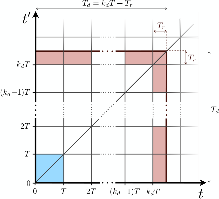
Starting from the general expression for the spectral density, Eq. (24), in this appendix we make the derivations required to turn it into the simplified expression (25) provided in the main text. In order to perform the two-time integral (24) we split the integration domain into intervals of duration , obtaining a kind of chessboard as shown in Fig. 4. We denote by the number of full periods contained in the detection interval, which is the common number of squares along the horizontal and the vertical directions of the chessboard, and by the remainder (, with and ), which is the width of the red boundaries in the figure. According to this, we decompose the integral (24), using Eq. (19), as
| (57) |
where the generic integral
| (58) | ||||
extends over the square whose lower-left corner seats at , and the remainder reads
| (59) | ||||
where
| (60a) | ||||
| (60b) | ||||
| (60c) | ||||
are integrals extending over the incomplete squares at the red boundary of the chessboard in Fig. 4, and we keep the same convention on the upper indices as with the integrals.
As we show next, the key point is that any of the above integrals, or , can be algebraically related to integrals defined over the domain, corresponding to the blue square in Fig. 4. Consider first the integrals of Eq. (58). Because takes on different expressions depending on whether or , see Eq. (20b), we must distinguish between integration domains that are above, below, or along the chessboard’s diagonal (also represented in Fig. 4). We then distinguish between integrals with , and integrals with and , which we will denote respectively as and . When , then , hence the argument of the noise correlation in Eq. (20b) is , while if , then , hence the argument is . Performing the variable change and in the integrals, using Eq. (20b), and recalling the assumed -periodicity of the functions , we get
| (61a) | ||||
| (61b) | ||||
where
| (62a) | ||||
| (62b) | ||||
Note that the “” operator has disappeared, as now integrals extend along . As for the integrals , we proceed along the previous lines, just considering that the argument of in Eq. (20b) is in the lower-right half of any diagonal square (which we denote by “” in the following), while it is in the upper-left one (which we denote by “ ”). Performing the variable change and , we then easily find that all integrals have the same value,
| (63) |
where
| (64a) | ||||
| (64b) | ||||
It is interesting to note that when the noise correlation matrix is symmetric, so that , these integrals satisfy the property .
With all previous results we can finally give a compact expression for the spectral density defined in Eq. (24). Substituting Eqs. (61) and (63) into Eq. (57), and performing the summations we obtain
| (65) | ||||
where was defined in Eq. (20a), and we have introduced the auxiliary function
| (66) | ||||
Note that when the detection time contains very many periods , i.e. when , the general expression (65) simplifies, since , , and the contribution of the remainder becomes negligible. Thus, in this this limit we obtain exactly the form that we presented in the main text, Eq. (25). Otherwise, the reminder needs to be evaluated, and for that it is useful to have an expression referred only to the first period. In order to do this, we simply proceed in the same manner as we did for the determination of the integrals , now taking into account that . The remainder defined in Eq. (59) can be reduced, after working out the summations, to
| (67) |
where the integral has been defined as in Eq. (60c), setting . Hence it formally coincides with in Eq. (58), with the substitution in Eqs. (64), and accordingly it is given by Eq. (63) with the latter substitution. We have also defined the following integrals
| (68a) | ||||
| (68b) | ||||
Appendix C Working out cross-correlations and cross-spectral densities with the noise
In this appendix we explain how we have dealt with the cross-correlations between the projections and the noise, as well as with the corresponding spectral density, in order to find the simplified expressions of Eqs. (30) and (31). Regarding the correlation functions, these are immediately found by using the solution (13) and the form of the projected noise (11b). In particular, we get
| (69) | ||||
which is precisely the expression (30) that we provide in the main text. Proceeding in the same way, one finds the expression for shown in (30).
As for the spectral density associated to , we simply need to note that this cross-correlation is zero in the upper triangular region of the integration domain of Fig. 4, while in the lower triangular it has the same form as in Eq. (52), just replacing by , where we have used the periodicity of and . Hence, it is clear that using the same derivations as in the previous appendix, in particular the ones turning Eq. (57) into Eq. (65), one obtains the spectral density introduced in (31) after taking the limit. A similar argument applies to the spectral density of the other cross-correlation , just noting that this one is zero in the lower triangular region of the integration domain of Fig. 4.
References
- (1) S. Ma, Z. Liao, F. Li, and M. S. Zubairi, EPL 110, 40004 (2015).
- (2) A. Kronwald, F. Marquardt, and A. A. Clerk, Phys. Rev. A 88, 063833 (2013).
- (3) E. E. Wollman et al., Science 349, 6251 (2015).
- (4) A. Mari and J. Eisert, Phys. Rev. Lett. 103, 213603 (2009).
- (5) A. Farace and V. Giovannetti, Phys. Rev. A 86, 013820 (2012).
- (6) A. Kronwald, F. Marquardt, and A. A. Clerk, New J. Phys. 16, 063058 (2014).
- (7) R. Garcés and G. J. de Valcárcel, Sci. Rep. 6, 21964 (2016).
- (8) B. A. Levitan, A. Metelmann, and A. A. Clerk, New J. Phys. 18, 093014 (2016).
- (9) A. Mari and J. Eisert, New J. Phys. 14, 075014 (2012).
- (10) C.-G. Liao, R.-X. Chen, H. Xie, and X.-M. Lin, Phys. Rev. A 97, 042314 (2018).
- (11) M. Abdi and M. J. Hartmann, New. J. Phys. 17, 013056 (2015).
- (12) X. Zhang, J. Sheng, and H. Wu, Opt. Express 26, 6285 (2018).
- (13) A. A. Clerk, F. Marquardt, and K. Jacobs, New J. Phys. 10, 095010 (2008).
- (14) D. Malz and A. Nunnenkamp, Phys. Rev. A 94, 053820 (2016).
- (15) M. A. Lemond, N. Didier, and A. A. Clerk, Nature Commun. 7, 11338 (2016).
- (16) I. Goychuk, J. Casado-Pascual, M. Morillo, J. Lehmann, and P. Hanggi, Phys. Rev. Lett. 97, 210601 (2006).
- (17) S. B. Shim, M. Imboden, and P. Mohanty, Science 316, 95 (2007).
- (18) O. V. Zhirov and D. L. Shepelyansky, Phys. Rev. Lett. 100, 014101 (2008).
- (19) M. Hossein-Zadeh and K. J. Vahala, Appl. Phys. Lett. 93, 191115 (2008).
- (20) T. E. Lee and H. R. Sadeghpour, Phys. Rev. Lett. 111, 234101 (2013).
- (21) S. Walter, A. Nunnenkamp, and C. Bruder, Phys. Rev. Lett. 112, 094102 (2014).
- (22) S. Y. Shah, M. Zhang, R. Rand, and M. Lipson, Phys. Rev. Lett. 114, 113602 (2015).
- (23) E. Amitai, N. Lörch, A. Nunnenkamp, S. Walter, and C. Bruder, Phys. Rev. A 95, 053858 (2017).
- (24) Ch. Bekker, R. Kalra, Ch. Baker, and W. P. Bowen, Optica 4, 1196 (2017).
- (25) L. Du, C.-H. Fan, H.-X. Zhang, and J.-H. Wu, Sci. Rep. 7, 15834 (2017).
- (26) G. Manzano, F. Galve, G. L. Giorgi, E. Hernández-García, and R. Zambrini, Sci. Rep. 3, 1439 (2013).
- (27) D. Witthaut, S. Wimberger, R. Burioni, and M. Timme, Nature Commun. 8, 14829 (2017).
- (28) C. Navarrete-Benlloch, J. J. García-Ripoll, and D. Porras, Phys. Rev. Lett. 113, 193601 (2014).
- (29) Z. Leghtas, S. Touzard, I. M. Pop, A. Kou, B. Vlastakis, A. Petrenko, K. M. Sliwa, A. Narla, S. Shankar, M. J. Hatridge, M. Reagor, L. Frunzio, R. J. Schoelkopf, M. Mirrahimi, and M. H. Devoret, Science 347, 853 (2015).
- (30) M. Benito, C. Sánchez Muñoz, and C. Navarrete-Benlloch, Phys. Rev. A 93, 023846 (2016).
- (31) A. Metelmann and H. E. Türeci, Phys. Rev. A 97, 043833 (2018).
- (32) A. Metelmann and A. A. Clerk, Phys. Rev. A 95, 013837 (2017).
- (33) K. Fang, J. Luo, A. Metelmann, M. H. Matheny, F. Marquardt, A. A. Clerk, O. Painter, Nature Physics 13, 465 (2017).
- (34) A. Kamal and A. Metelmann, Phys. Rev. Applied 7, 034031 (2017).
- (35) F. Lecocq, L. Ranzani, G. A. Peterson, K. Cicak, A. Metelmann, S. Kotler, R. W. Simmonds, J. D. Teufel, and J. Aumentado, Phys. Rev. Appl. 13, 044005 (2020).
- (36) C. Arenz and A. Metelmann, Phys. Rev. A 101, 022101 (2020).
- (37) A. Metelmann and A. A. Clerk, Phys. Rev. X 5, 021025 (2015).
- (38) T. J. Kippenberg, H. Rokhsari, T. Carmon, A. Scherer, and K. J. Vahala, Phys. Rev. Lett. 95, 033901 (2005).
- (39) T. Carmon, H. Rokhsari, L. Yang, T. J. Kippenberg, and K. J. Vahala, Phys. Rev. Lett. 94, 223902 (2005).
- (40) C. Metzger, M. Ludwig, C. Neuenhahn, A. Ortlieb, I. Favero, K. Karrai, and F. Marquardt, Phys. Rev. Lett. 101, 133903 (2008).
- (41) G. Anetsberger et al., Nature Phys. 5, 909 (2009).
- (42) F. Marquardt, J. G. E. Harris, and S. M. Girvin, Phys. Rev. Lett. 96, 103901 (2006).
- (43) J. B. Khurgin, M. W. Pruessner, T. H. Stievater, and W. S. Rabinovich, Phys. Rev. Lett. 108, 223904 (2012).
- (44) J. B. Khurgin, M. W. Pruessner, T. H. Stievater, and W. S. Rabinovich, New J. Phys. 14, 105022 (2012).
- (45) M. Ludwig, B. Kubala, and F. Marquardt, New J. Phys. 10, 095013 (2008).
- (46) D. A. Rodrigues and A. D. Armour, Phys. Rev. Lett. 104, 053601 (2010).
- (47) J. Qian, A. A. Clerk, K. Hammerer, and F. Marquardt, Phys. Rev. Lett. 109, 253601 (2012).
- (48) N. Lörch, J. Qian, A. Clerk, F. Marquardt, and K. Hammerer, Phys. Rev. X 4, 011015 (2014).
- (49) G. Wang, L. Huang, Y.-C. Lai, and C. Grebogi, Phys. Rev. Lett. 112, 110406 (2014).
- (50) C. Navarrete-Benlloch, T. Weiss, S. Walter, and G. J. de Valcárcel, Phys. Rev. Lett. 119, 133601 (2017).
- (51) A. Chia, L. C. Kwek, and C. Noh, Phys. Rev. E 102, 042213 (2020).
- (52) E. T. Owen, J. Jin, D. Rossini, R. Fazio, and M. J. Hartmann, New J. Phys. 20, 045004 (2018).
- (53) S. Khan and H. E. Türeci, Phys. Rev. Lett. 120, 153601 (2018).
- (54) A. Chia, M. Hajdušek, R. Nair, R. Fazio, L. C. Kwek, V. Vedral, Phys. Rev. Lett. 125, 163603 (2020).
- (55) A. Chia, M. Hajdušek, R. Fazio, L. C. Kwek, V. Vedral, Quantum 3, 200 (2019).
- (56) F. Wilczek, Scientific American 321, 28 (2019).
- (57) F. Wilczek, Phys. Rev. Lett. 109, 160401 (2012).
- (58) A. Shapere and F. Wilczek, Phys. Rev. Lett. 109, 160402 (2012).
- (59) V. Khemani, R. Moessner, and S. L. Sondhi, arXiv:1910.10745.
- (60) A. Russomanno, F. Iemini, M. Dalmonte, and R. Fazio, Phys. Rev. B 95, 214307 (2017).
- (61) F. Iemini, A. Russomanno, J. Keeling, M. Schirò, M. Dalmonte, and R. Fazio, Phys. Rev. Lett. 121, 035301 (2018).
- (62) B. Zhu, J. Marino, N. Y. Yao, M. D. Lukin, and E. A. Demler, New J. Phys. 21, 073028 (2019).
- (63) A. Lazarides, S. Roy, F. Piazza, and R. Moessner, Phys. Rev. Research 2, 022002(R) (2020).
- (64) L. Droenner, R. Finsterhölzl, M. Heyl, and A. Carmele, arXiv:1902.04986.
- (65) Z. Cai, Y. Huang, and W. V. Liu, Chin. Phys. Lett. 37, 050503 (2020) (Express letter).
- (66) H. Keßler, J. G. Cosme, M. Hemmerling, L. Mathey, and A. Hemmerich, Phys. Rev. A 99, 053605 (2019).
- (67) H. Keßler, J. G. Cosme, C. Georges, L. Mathey, and A. Hemmerich, arXiv:2004.14633.
- (68) D. V. Else, C. Monroe, C. Nayak, and N. Y. Yao, arXiv:1905.13232.
- (69) N. Yao and C. Nayak, Physics Today 71, 9, 40 (2018).
- (70) K. Sacha and J. Zakrzewski, Rep. Prog. Phys. 81, 016401 (2018).
- (71) L. Guo and P. Liang, arXiv:2005.03138.
- (72) K. Sacha, Phys. Rev. A 91, 033617 (2015).
- (73) V. Khemani, A. Lazarides, R. Moessner, and S. L. Sondhi, Phys. Rev. Lett. 116, 250401 (2016).
- (74) D. V. Else, B. Bauer, and C. Nayak, Phys. Rev. Lett. 117, 090402 (2016).
- (75) C. W. von Keyserlingk, V. Khemani, and S. L. Sondhi, Phys. Rev. B 94, 085112 (2016).
- (76) N. Y. Yao, A. C. Potter, I. D. Potirniche, and A. Vishwanath, Phys. Rev. Lett. 118, 030401 (2017).
- (77) J. Zhang, P. W. Hess, A. Kyprianidis, P. Becker, A. Lee, J. Smith, G. Pagano, I. D. Potirniche, A. C. Potter, A. Vishwanath, N. Y. Yao, and C. Monroe, Nature 543, 217 (2017).
- (78) S. Choi, J. Choi, R. Landi, G. Kucsko, H. Zhou, J. Isoya, F. Jelezko, S. Onoda, H. Sumiya, V. Khemani, C. von Keyserlingk, N. Y. Yao, E. Demler, and M. D. Lukin, Nature 543, 221 (2017).
- (79) J. Rovny, R. L. Blum, and S. E. Barrett, Phys. Rev. Lett. 120, 180603 (2018).
- (80) J. Rovny, R. L. Blum, and S. E. Barrett, Phys. Rev. B 97, 184301 (2018).
- (81) S. Pal, N. Nishad, T. S. Mahesh, and G. J. Sreejith, Phys. Rev. Lett. 120, 180602 (2018).
- (82) J. Smits, L. Liao, H. T. C. Stoof, and P. van der Straten, Phys. Rev. Lett. 121, 185301 (2018).
- (83) S. Autti, V. B. Eltsov, and G. E. Volovik, Phys. Rev. Lett. 120, 215301 (2018).
- (84) C. Georges, J. G. Cosme, H. Keßler, L. Mathey, A. Hemmerich, arXiv:2003.14135.
- (85) M. P. Estarellas, T. Osada, V. M. Bastidas, B. Renoust, K. Sanaka, W. J. Munro, K. Nemoto, Sci. Adv. 6, EAAY8892 (2020).
- (86) J. H. Shirley, Phys. Rev. 138, B979 (1965).
- (87) M. Grifoni and P. Hänggi, Phys. Rep. 304, 229 (1998).
- (88) T. Oka and S. Kitamura, Ann. Rev. Cond. Matt. Phys. 10, 387 (2018).
- (89) P. D. Drummond and C. W. Gardiner, J. Phys. A 13, 2353 (1980).
- (90) C. W. Gardiner and P. Zoller, Quantum Noise (Springer-Verlag, Heidelberg, 1991).
- (91) A. Gilchrist, C. W. Gardiner, and P. D. Drummond, Phys. Rev. A 55, 3014 (1997).
- (92) C. Navarrete-Benlloch, Ph.D. thesis, Universitat de València, 2011; arXiv:1504.05917.
- (93) C. Navarrete-Benlloch, E. Roldán, and G. J. de Valcárcel, Phys. Rev. Lett. 100, 203601 (2008).
- (94) C. Navarrete-Benlloch, G. J. de Valcárcel, and E. Roldán, Phys. Rev. A 79, 043820 (2009).
- (95) C. Navarrete-Benlloch, A. Romanelli, E. Roldán, and G. J. de Valcárcel, Phys. Rev. A 81, 043829 (2010).
- (96) C. Navarrete-Benlloch, G. Patera, and G. J. de Valcárcel, Phys. Rev. A 96, 043801 (2017).
- (97) C. Navarrete-Benlloch, E. Roldán, Y. Chang, and T. Shi, Opt. Express 22, 024010 (2014).
- (98) P. Degenfeld-Schonburg, C. Navarrete-Benlloch, and M. J. Hartmann, Phys. Rev. A 91, 053850 (2015).
- (99) M. Aspelmeyer, T. J. Kippenberg, and F. Marquardt, Rev. Mod. Phys. 86, 1391 (2014).
- (100) D. Malz and A. Nunnenkamp, Phys. Rev. A 94, 023803 (2016).
- (101) E. B. Aranas, M. J. Akram, D. Malz, and T. S. Monteiro, Phys. Rev. A 96, 063836 (2017).
- (102) G. Floquet, Ann. Sci. ENS 12, 47 (1883).
- (103) V. A. Yakubovich and V. M. Starzhinskii, Linear differential equations with periodic coefficients, Volume 1 (Wiley, New York, 1975).
- (104) R. Grimshaw, Nonlinear Ordinary Differential Equations (Blackwell Scientific, London, 1990).
- (105) E. A. Coddington and N. Levinson, Theory of Ordinary Differential Equations (McGraw-Hill, New York, 1955).
- (106) F. Haddadfarshi, J. Cui, and F. Mintert, Phy. Rev. Lett. 114, 130402 (2015).
- (107) C. M. Dai, Z. C. Shi, and X. X. Yi, Phys. Rev. A 93, 032121 (2016).
- (108) C. Navarrete-Benlloch, An Introduction to the Formalism of Quantum Information with Continuous Variables (Morgan & Claypool and IOP, Bristol, 2015).
- (109) J. Gea-Banacloche, N. Lu, L. M. Pedrotti, S. Prasad, M. O. Scully, and K. Wodkiewicz, Phys. Rev. A 41, 369 (1990).
- (110) B. Kühn, W. Vogel, M. Mraz, S. Köhnke, and B. Hage, Phys. Rev. Lett. 118, 153601 (2017).
- (111) G. Patera, N. Treps, C. Fabre, and G. J. de Valcárcel, Eur. Phys. J. D 56, 123 (2010).
- (112) C. Zerbe and P. Hänggi, Phys. Rev. E 52, 1533 (1995)
- (113) S. Kohler, T. Dittrich, and P. Hänggi, Phys. Rev. E 55, 300 (1997).
- (114) M. Thorwart, P. Reimann, and P. Hänggi, Phys. Rev. E 62, 5808 (2000).
- (115) É. Gouzien , S. Tanzilli, V. D’Auria, and G. Patera, Phys. Rev. Lett. 125, 103601 (2020).