BART-based inference for Poisson processes
Abstract
The effectiveness of Bayesian Additive Regression Trees (BART) has been demonstrated in a variety of contexts including non-parametric regression and classification. A BART scheme for estimating the intensity of inhomogeneous Poisson processes is introduced. Poisson intensity estimation is a vital task in various applications including medical imaging, astrophysics and network traffic analysis. The new approach enables full posterior inference of the intensity in a non-parametric regression setting. The performance of the novel scheme is demonstrated through simulation studies on synthetic and real datasets up to five dimensions, and the new scheme is compared with alternative approaches.
1 Introduction
The Bayesian Additive Regression Trees (BART) model is a Bayesian framework, which uses a sum of trees to predict the posterior distribution of a response given a -dimensional covariate and priors on the function relating the covariates to the response. Chipman et al. 2010 proposed an inference procedure using Metropolis Hastings within a Gibbs Sampler, whereas Lakshminarayanan et al. 2015 used a Particle Gibbs Sampler to increase mixing when the true posterior consists of deep trees or when the dimensionality of the data is high. Several theoretical studies of BART models (Rockova and van der Pas 2017; Rockova and Saha 2018; Linero and Yang 2018) have recently established optimal posterior convergence rates. The BART model has been applied in various contexts including non-parametric mean regression (Chipman et al. 2010), classification (Chipman et al. 2010; Zhang and Härdle 2010; Kindo et al. 2016), variable selection(Chipman et al. 2010; Bleich et al. 2014; Linero 2018), estimation of monotone functions (Chipman et al. 2021), causal inference (Hill 2011), survival analysis (Sparapani et al. 2016), and heteroskedasticity (Bleich and Kapelner 2014; Pratola et al. 2020). Linero and Yang 2018 illustrated how the BART model suffers from a lack of smoothness and the curse of dimensionality, and overcome both potential shortcomings by considering a sparsity assumption similar to (Linero 2018) and treating decisions at branches probabilistically.
The original BART model (Chipman et al. 2010) assume that the response has a Gaussian distribution and the majority of applications have used this framework. Murray 2017 adapted the BART model to count data and categorical data via a log-linear transformation, and provided an efficient MCMC sampler. Our focus is on extending this methodology to estimate the intensity function of inhomogeneous Poisson processes.
The question of estimating the intensity of Poisson processes has a long history, including both frequentist and Bayesian methods. Frequentist methods include fixed-bandwidth and adaptive bandwidth kernel estimators with edge correction (Diggle et al. 2003), and wavelet-based methods (Fryzlewicz and Nason 2004; Patil et al. 2004, e.g. ). Bayesian methods include using a sigmoidal Gaussian Cox process model for intensity inference (Adams et al. 2009), a Markov random field (MRF) with Laplace prior (Sardy and Tseng 2004), variational Bayesian intensity inference (Lloyd et al. 2015), and non-parametric Bayesian estimations of the intensity via piecewise functions with either random or fixed partitions of constant intensity (Arjas and Gasbarra 1994; Heikkinen and Arjas 1998; Gugushvili et al. 2018).
In this paper, we introduce an extension of the BART model (Chipman et al. 2010) for Poisson Processes whose intensity at each point is estimated via a tiny ensemble of trees. Specifically, the logarithm of the intensity at each point is modelled via a sum of trees (and hence the intensity is a product of trees). This approach enables full posterior inference of the intensity in a non-parametric regression setting. Our main contribution is a novel BART scheme for estimating the intensity of an inhomogeneous Poisson process. The simulation studies demonstrate that our algorithm is competitive with the Haar-Fisz algorithm in one dimension, kernel smoothing in two dimensions, and outperforms the kernel approach for multidimensional intensities. The simulation analysis also demonstrates that our proposed algorithm is competitive with the inference via spatial log-Gaussian Cox processes. We also demonstrate its ability to track varying intensity in synthetic and real data.
The outline of the article is as follows. Section 2 introduces our approach for estimating the intensity of a Poisson process through the BART model, and Section 3 presents the proposed inference algorithm. Sections 4 and 5 present the application of the algorithm to synthetic data and real data sets, respectively. Section 6 provides our conclusions and plans for future work.
2 The BART Model for Poisson Processes
Consider an inhomogeneous Poisson process defined on a -dimensional domain , , with intensity . For such a process, the number of points within a subregion has a Poisson distribution with mean , and the number of points in disjoint subregions are independent (Daley and Vere-Jones 2003). The homogeneous Poisson process is a special case with constant intensity .
To estimate the intensity of the inhomogeneous Poisson process, we use partitions of the domain , each associated with a tree . The partitions are denoted , where is the number of terminal nodes in the corresponding tree , and each leaf node corresponds to one of the subregions of the partition . Being a partition, every tree covers the full domain, i.e. for every . Each subregion has an associated parameter , and hence each tree has an associated vector of leaf intensities .
We model the intensity of as:
| (1) | ||||
| (2) | ||||
| (3) |
where denotes the indicator function. Equivalently, (1) can be expressed as
| (4) |
Given a fixed number of trees, , the parameters of the model are thus the regression trees and their corresponding intensities . Following Chipman et al. 2010, we assume that the tree components are independent of each other, and that the terminal node parameters of every tree are independent, so that the prior can be factorized as:
| (5) |
Prior on the trees
The trees of the BART model are stochastic regression trees generated through a heterogeneous Galton-Watson (GW) process (Harris et al. 1963; Rockova and Saha 2018). The GW process is the simplest branching process concerning the evolution of a population in discrete time. Individuals (tree nodes) of a generation (tree depth) give birth to a random number of individuals (tree nodes), called offspring, mutually independent and all with the same offspring distribution that may vary from generation (depth) to generation (depth). In our case, we use the prior introduced by Chipman et al. 1998, that is a GW process in which each node has either zero or two offspring and the probability of a node splitting depends on its depth in the tree. Specifically, a node splits into two offsprings with probability
| (6) |
where is the depth of node in the tree, and and are parameters of the model. Classic results from the theory of branching processes show that guarantees that the expected depth of the tree is finite. In our construction, each tree is associated with a partition of . Namely, if node splits, we select uniformly at random one of the dimensions of the space of the Poisson process, followed by uniform selection from the available split values associated with that dimension respecting the splitting rules higher in the tree.
Prior on the leaf intensities
Our choice of a Gamma prior for the leaf parameters builds upon previous work by Murray 2017, who used a mixture of Generalized Inverse Gaussian (GIG) distributions as the prior on leaf parameters in a BART model for count regression. Here we impose a Gamma prior (a special case of GIG) on the leaf parameters, which simplifies the model and leads to a closed form of the conditional integrated likelihood below (see Section 3) as the Gamma distribution is the conjugate prior for the Poisson likelihood. We discuss the selection of it hyperparameters and in Section 3.1.
3 The Inference Algorithm
Given a finite realization of an inhomogeneous Poisson process with sample points , we seek to infer the parameters of the model by sampling from the posterior .
Before presenting the sampling algorithm we summarize a preliminary result. To simplify our notation, let us define
so that Eq. (4) becomes .
Let us choose any arbitrary tree in our ensemble , and let us denote the set with the rest of the trees as and their leaf parameters as . The intersection of all the partitions associated with the trees in gives us a global partition with subregions (Rockova and van der Pas 2017).
Then we have the following result.
Remark 1.
- (i)
The conditional likelihood of the realization is given by
(7) where , is the cardinality of the set , and is the volume of the region .
- (ii)
For a tree , the conditional integrated likelihood obtained by integrating out is
(8)
We now summarize our sampling algorithm. To sample from , we implement a Metropolis-Hastings within block Gibbs sampler (Algorithm 1), which requires successive draws from . Note that
| (9) |
which follows directly from Bayes’ rule and Eqs. (5) and (3).
From (), it is clear that a draw from can be achieved in (+1) successive steps consisting of:
- •
sampling using Metropolis-Hastings (Algorithm 2)
- •
sampling from a Gamma distribution with shape and rate for .
These steps are implemented through Metropolis-Hastings in Algorithm 1. Note also that
so that the conditional integrated likelihood (8) is required to compute the Hastings ratio.
The transition kernel in Algorithm 2 is chosen from the three proposals: GROW, PRUNE, CHANGE (Chipman et al. 2010; Kapelner and Bleich 2013). The GROW proposal randomly picks a terminal node, splits the chosen terminal into two new nodes and assigns a decision rule to it. The PRUNE proposal randomly picks a parent of two terminal nodes and turns it into a terminal node by collapsing the nodes below it. The CHANGE proposal randomly picks an internal node and randomly reassigns to it a splitting rule. We describe the implementation of the proposals in A.
For completeness, in the supplementary material, we present the full development of the algorithm for inference of the intensity of inhomogeneous Poisson processes via only one tree.
3.1 Fixing the hyperparameters of the model
Hyperparameters of the Gamma distribution for the leaf intensities
We use a simple data-informed approach to fix the hyperparameters and of the Gamma distribution (3). We discretize the domain into subregions of equal volume ( works well in practice up to 5 dimensions) and count the number of samples per subregion. We thus obtain the empirical densities in each of the subregions: . Given the form of the intensity (4) as a product of trees, we consider the -th roots as candidates for the intensity of each tree. Taking the sample mean and sample variance , we choose the model hyperparameters and to correspond to those of a Gamma distribution with the same mean and variance, i.e., and , although fixing can also give good estimates of the intensity. Although setting leads to convergence and good estimates of the intensity in our simulation studies below, there are other possibilities. Alternatively, we can bin the data based on a criterion that takes into account the number of samples, , and the number of dimensions, . For example, the number of bins per dimension, , can be computed as (Scott 2008; Wand 1997): (i) , (ii) , or (iii) , where IQR denotes the interquartile range of the sample, is the range of the domain in dimension (here we scale the initial domain to a unit hypercube so that ), and by extension . In our simulation scenarios below, all these approaches lead to comparable convergence times and estimates of the intensity.
Hyperparameters of the stochastic ensemble of regression trees
The GW stochastic process that generates our tree ensemble has several hyperparameters. The parameters control the shape of trees. The parameter controls the probability that the root of a tree will split into two offspring, while the parameter penalizes against deep trees. As noted in (Chipman et al. 2010), for a sum-of-trees model, we want to keep the depth of the tree small whilst ensuring non-trivial trees, hence, in our simulation study we fix and . Second, each of the dimensions has to be assigned a grid of split values, from which the subregions of the partition are randomly chosen, yet always respecting the consistency of the ancestors in the tree (that is respecting the splitting rules higher in the tree). Here, we use a simple uniform grid for each of the -dimensions (Pratola et al. 2016): we normalize each dimension of the space from (0,1) and discretize each dimension into segments. ( works well in practice and is used throughout our examples.) More sophisticated, data-informed grids are also possible, although using, e.g., the sample points as split values does not improve noticeably the performance in our examples. Finally, the number of trees also needs to be fixed as in Chipman et al. 2010. In our examples below, we have checked the performance of our algorithm with varying number of trees between 2 and 50. We find that good performance can be achieved with a moderate number of trees, , between 3 and 10 depending on the particular example.
4 Simulation Study on Synthetic Data
We carried out a simulation study on synthetic data to illustrate the performance of Algorithm 1 to estimate first the intensity of one dimensional and two dimensional inhomogeneous Poisson processes and finally the intensity of multidimensional Poisson processes.
We simulate realizations of Poisson processes on the domain for via thinning (Lewis and Shedler 1979). The hyperparameters of the model (for the trees and the leaf intensities) are fixed as described in Section 3.1. We initially randomly generate trees of zero depth. The probabilities of the proposals in Algorithm 2 are set to: and . A set is defined by uniformly sampling points in the domain .
We run 3 parallel chains of the same length. We discard their first halves treating the second halves as a sample from the target distribution. We assess chain convergence using the Gelman-Rubin convergence diagnostic (Gelman et al. 1992) applied to the estimated intensity for each point of the set , as well as trace plots and autocorrelation plots for some points of the testing set.
At each state of a simulated chain we estimate the intensity for each point by a product of trees denoted as
The induced sequence for the sequence of draws converges to . We estimate the posterior mean , the posterior median of , and the highest density interval (hdi) using the function provided by the R package bayestestR (Makowski et al. 2019). To assess the performance of our algorithm, we compute the Average Absolute Error (AAE) of the computed estimate:
| (11) |
and the Root Integrated Square Error (RISE):
| (12) |
where is the number of test points.
In the spirit of Akaike information criterion (AIC) (Loader 1999), we also introduce two diagnostics targetting the likelihood function to evaluate if increasing the number of trees leads to better intensity estimation:
and
where is the number of global cells, and is the overall number of leaves in the ensemble. We estimate both diagnostics using the sequence of the draws after the burn-in period as
and
where and are the number of global cells and the overall number of leaves in the ensemble associated to the draw, respectively.
AIC has been shown to be asymptomatically equal to leave-one-out cross validation (LOO-CV) (Stone 1977; Gelman et al. 2014). According to Leininger and Gelfand 2017, the computational burden required for leave-one-out cross validation considering a point pattern data is impractical. We introduce a leave-partition-out (LPO) method, assuming that the initial process is obtained by combining independent processes , as follows
| (13) |
where is the leave-partition-out predictive intensity given the process without the partition, . We can evaluate 13 as follows,
where is the sequence of draws after the burn-in period leaving out the partition . We assume that each event of is coming from with probability . The bias of the method is introduced by randomly splitting the process into individual processes. We can get the LOO-CV by LPO, defining appropriately the parameter . As higher the number is, as less biased the method is. In the simulation scenarios, we consider that , and for computational reasons. The diagnostics show that tiny ensembles of trees provide good estimates in our simulation scenarios.
To confirm the proposed diagnostics, we use -thinning (Illian et al. 2008, Chapter 6) with to create training and test datasets in two of the simulation scenarios. We employ Root Standardized Mean Square Error (RSMSE) and Rank Probability Score (RPS) with the test data set comparing observed counts in disjoint equal volume subregions as follows:
| (14) |
and
| (15) |
where is the Poisson distribution with parameter , the actual number of testing points in and the estimated number of testing points in given by
| (16) |
with being the number of points falling in and estimating the intensity at each points , , via the posterior mean .
For one dimensional processes, we compare the results of Algorithm 1 to the Haar-Fisz algorithm (Fryzlewicz and Nason 2004), a wavelet based method for estimating the intensity of one dimensional Poisson Processes that outperforms well known competitors. We apply the Haar-Fisz algorithm to the counts of points falling into 256 consecutive intervals using the R package haarfisz (Fryzlewicz 2010). Our algorithm is competitive with the Haar algorithm for smooth intensity functions and is not strongly out-performed by the Haar-Fisz algorithm when the underlying intensity is a stepwise function.
For two-dimensional processes, we compare the results of our algorithm with fixed-bandwidth estimators and log-Gaussian Cox processes (LGCP) with intensity where is a Gaussian process with exponential covariance function. We used a discretization version of the LGCP model defined on a regular grid over space which we implemented using Stan-code (Gelman et al. 2015). As noted in Davies and Baddeley 2018, the choice of the kernel is not of primary importance, we choose a Gaussian kernel for its wide applicability. In our tables of results, the smoothing bandwidth, sigma, selected using likelihood cross-validation (Loader 1999) denoted by (LCV), and we have also included other values of sigma to demonstrate the sensitivity to bandwidth choice. The kernel estimators, and the bandwidth value given by likelihood cross-validation, were computed using the R package spatstat (Baddeley and Turner 2005). Our algorithm outperforms the maximum likelihood approach using linear conditional intensity, as expected. Our algorithm outperforms kernel smoothing and LGCP for stepwise functions and is competitive with them for a smooth intensity.
Finally, we examine the performance of our algorithm for multidimensional intensities by generating realizations of Poisson Processes on the domain for via thinning. Future work includes the study of intensities in higher dimensions (). We compare our intensity estimates with kernel smoothing estimators having isotropic standard deviation matrices with diagonal elements equal to and the methodology for applying maximum likelihood to point process models with linear conditional intensity (Peng 2003). We select the bandwidth using likelihood cross-validation (Loader 1999) denoted by (LCV).
4.1 One dimensional Poisson Process with stepwise intensity
Our first example is a one dimensional Poisson Process with piecewise constant intensity with several steps (Fig. 1). We run 3 parallel chains of the same length for 200000 iterations for 2-10 trees, 100000 for 12 trees, 50000 iterations for 15 trees and 30000 iterations for 20 trees.
Our algorithm detects the change points and provides good estimates of the intensity and is competitive in terms of AAE with the Haar-Fisz algorithm, but does not perform as well in terms of RISE (see Fig. 1 and Tables 3-6). We have found the metrics and convergence diagnostics in a set of uniformly chosen points without excluding the points close to jumps. Due to inferring the intensity via a product of stepwise functions, it is expected that the proposed algorithm will provide estimates with higher variability close to jumps. The proposed algorithm outperforms the Haar-Fisz algorithm without considering the points close to jumps. Tables 4-5 show the metrics for various number of trees without considering the points in a distance from the jumps.
The diagnostics , and obtain their highest values for 7, 4 and 8 trees, respectively. The analysis demonstrates only small differences between log-likelihood values as the number of trees increases, supporting results found in previous BART studies that the method is robust to the choice of . The average RSMSE and RPS on testing points over 7 different splits of the original data set (Tables 1-2) provide evidence that ensembles with more than seven trees do not improve the fit of the proposed algorithm.
| Proposed BART Algorithm | ||||||
|---|---|---|---|---|---|---|
| Number of trees | ||||||
| 2 | 17.05 | 5.24 | 3.10 | 2.08 | 1.66 | 1.44 |
| 3 | 17.12 | 5.25 | 3.11 | 2.08 | 1.65 | 1.43 |
| 4 | 16.98 | 5.28 | 3.09 | 2.07 | 1.64 | 1.42 |
| 5 | 16.94 | 5.26 | 3.04 | 2.06 | 1.63 | 1.41 |
| 7 | 17.01 | 5.22 | 3.00 | 2.04 | 1.62 | 1.40 |
| 8 | 17.09 | 5.20 | 2.99 | 2.03 | 1.62 | 1.40 |
| 9 | 17.07 | 5.20 | 2.98 | 2.02 | 1.61 | 1.39 |
| 10 | 20.10 | 5.78 | 3.12 | 2.12 | 1.63 | 1.43 |
| 12 | 17.74 | 5.37 | 2.99 | 2.06 | 1.63 | 1.39 |
| 15 | 17.03 | 5.15 | 2.94 | 2.01 | 1.60 | 1.38 |
| 20 | 17.08 | 5.16 | 2.93 | 2.00 | 1.60 | 1.38 |
| Proposed BART Algorithm | ||||||
|---|---|---|---|---|---|---|
| Number of trees | ||||||
| 2 | 0.95 | 1.13 | 1.06 | 1.02 | 0.99 | 1.00 |
| 3 | 0.95 | 1.13 | 1.06 | 1.02 | 0.98 | 0.99 |
| 4 | 0.95 | 1.14 | 1.06 | 1.02 | 0.98 | 0.98 |
| 5 | 0.94 | 1.13 | 1.04 | 1.02 | 0.98 | 0.98 |
| 7 | 0.95 | 1.13 | 1.04 | 1.01 | 0.97 | 0.97 |
| 8 | 0.95 | 1.12 | 1.03 | 1.01 | 0.97 | 0.96 |
| 9 | 0.95 | 1.13 | 1.03 | 1.01 | 0.97 | 0.97 |
| 10 | 1.10 | 1.20 | 1.06 | 1.04 | 0.98 | 0.98 |
| 12 | 0.98 | 1.18 | 1.04 | 1.02 | 0.98 | 0.96 |
| 15 | 0.95 | 1.12 | 1.02 | 1.00 | 0.97 | 0.96 |
| 20 | 0.95 | 1.12 | 1.02 | 1.00 | 0.97 | 0.96 |
| Proposed BART Algorithm | |||||||
|---|---|---|---|---|---|---|---|
| Number of trees | AAE for Posterior Mean | AAE for Posterior Median | RISE for Posterior Mean | RISE for Posterior Median | |||
| 3 | 308.87 | 320.84 | 603.54 | 633.48 | 54095.1 | 54090 | -339.7 |
| 4 | 287.89 | 283.03 | 580.69 | 587.08 | 54096.5 | 54090 | -368 |
| 5 | 289.27 | 281.13 | 580.55 | 586.24 | 54098 | 54088.4 | -352.5 |
| 7 | 281.59 | 274.88 | 588.7 | 592.11 | 54098 | 54082.7 | -263.5 |
| 8 | 280.62 | 274.07 | 588.73 | 591.29 | 54097.9 | 54079.5 | -261.5 |
| 9 | 282.78 | 276.99 | 593.93 | 595.23 | 54096.9 | 54075.2 | -327.9 |
| 10 | 283.79 | 279.07 | 593.95 | 595.41 | 54095.6 | 54071.6 | -322.6 |
| 20 | 297.21 | 287.86 | 599.77 | 595.04 | 54082.9 | 54029.7 | -436 |
| Proposed BART Algorithm | ||||
| Number of trees | AAE for Posterior Mean | AAE for Posterior Median | RISE for Posterior Mean | RISE for Posterior Median |
| 4 | 144.48 | 139.58 | 181.21 | 174.82 |
| 5 | 144.55 | 139.02 | 180.74 | 176.19 |
| 7 | 124.53 | 123.2 | 175.74 | 172.4 |
| Haar-Fisz Algorithm | |
|---|---|
| AAE | RISE |
| 141.95 | 192.6 |
| Haar-Fisz Algorithm | |
|---|---|
| AAE | RISE |
| 272.3 | 476.9 |
4.2 Two-dimensional Poisson process with stepwise intensity function
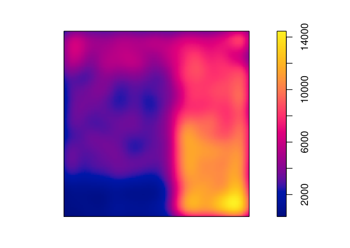
To demonstrate the applicability of our algorithm in a two-dimensional setting, Figures 2-3 and Tables 7-9 reveal that our algorithm outperforms kernel smoothing and inference with spatial log-Gaussian Cox processes for stepwise intensity functions. We run 3 parallel chains of the same length for 100000 iterations for 3-6 trees. The convergence criteria indicate convergence of the simulated chains for the majority of points. As may be expected, the simulation study shows that points close to jumps are estimated with less reliability. The algorithm converges less well at these points, as demonstrated by the Gelman-Rubin diagnostic (see supplementary material). The diagnostics , and obtain their highest values for three trees, respectively. The diagnostics indicate that small ensembles of trees can provide a good estimate of the intensity.



| Proposed BART Algorithm | |||||||
| Number of trees | AAE for Posterior Mean | AAE for Posterior Median | RISE for Posterior Mean | RISE for Posterior Median | |||
| 3 | 224.1 | 230.3 | 419.2 | 453.7 | 87227.2 | 87232.3 | 505.1 |
| 4 | 208.7 | 213 | 410.2 | 447.9 | 87223.7 | 87230.5 | 491.2 |
| 5 | 216.8 | 212.9 | 389.5 | 410.9 | 87211.6 | 87220.6 | 406 |
| 6 | 228.9 | 221.9 | 395.8 | 412.8 | 87197.5 | 87214.7 | 463.9 |
| Kernel Smoothing | ||
|---|---|---|
| Bandwidth (sigma) | AAE | RISE |
| 0.027 | 763.8 | 1041.3 |
| 0.038 | 662.7 | 956.8 |
| 0.047 (LCV) | 636.7 | 960.6 |
| 0.067 | 672.8 | 1042.5 |
| Inference with spatial log-Gaussian Cox processes | ||
| grid | AAE | RISE |
| 568 | 751 | |
| 678 | 953 | |
4.3 Inhomogeneous three-dimensional Poisson Process with Gaussian intensity
Our first example for multidimensional intensities is a three-dimensional Poisson process with intensity for . We generated a realization of 1616 points via thinning. We run 3 parallel chains of the same length for 100000 iterations for 3-10 trees and 30000 iterations for 12 trees. Tables 10 and 11 illustrate the statistics of our algorithm and kernel smoothing. Figures 4 and 5 show our estimators and the kernel estimator with =0.073 for 8 Trees and 10 Trees with fixed third dimension () at 0.4 and 0.8, respectively.
The diagnostics , and get their highest values with 4 trees, respectively. We observe that the diagnostic slightly differs between 4 and 8 trees. The diagnostic is similar between 4 and 5 trees. The estimate of the average logarithm of Poisson process likelihood does not change significantly from 4 trees to 12 trees. Specifically, we observe its maximum equal to 10536.3 at 12 trees, while its minimum to 10531.9 at 4 trees. In addition, the estimated average number of leaves in a tree of an ensemble is about 3 for trees. That explains why we observe higher values of diagnostics for a small number of trees. The metrics and are optimised with 12 trees. However, it should be noted that only small variations in the metrics are seen between 4 and 12 trees. The diagnostics provide evidence that increasing the number of trees does not improve the fit of the proposed model.
| Proposed BART Algorithm | |||||||
| Number of trees | AAE for Mean | AAE for Median | RISE for Mean | RISE for Median | |||
| 4 | 247.6 | 254.9 | 360.7 | 376.3 | 20993.7 | 21040.6 | -1409 |
| 5 | 250.2 | 258.3 | 364.3 | 380.4 | 20992.1 | 21039.8 | -1492 |
| 6 | 247.6 | 254.7 | 360.8 | 375.4 | 20979.5 | 21038.6 | -1529 |
| 8 | 234.8 | 239.4 | 341 | 352.4 | 20938.6 | 21032.8 | -1515 |
| 10 | 226.8 | 229.4 | 330.5 | 338.5 | 20883 | 21026.9 | -1539 |
| 12 | 221.6 | 222.3 | 320.6 | 326.4 | 20810.4 | 21020.7 | -1609 |
| Kernel Smoothing | ||
|---|---|---|
| AAE | RISE | |
| 0.053 | 480.8 | 667.5 |
| 0.073 (LCV) | 415.86 | 645.16 |
| 0.08 | 417.7 | 661.4 |
| 0.085 | 423.2 | 676.2 |
| 0.1 | 450.3 | 727.6 |
| 0.3 | 890.4 | 1236 |


4.4 Inhomogeneous five dimensional Poisson Process with sparsity assumption
Here, we demonstrate the performance of our algorithm to detect the dimensions that contribute most in the intensity of in a noisy environment. Consider a five dimensional inhomogeneous Poisson process with intensity function of depending on 3 of 5 dimensions:
We generate a realization of 669 points via thinning. We run 3 parallel chains of the same length for 100000 iterations for 4-8 trees, 50000 iterations for 10 trees, 30000 iterations for 12 trees and 10000 iterations for 15 trees. The convergence criterion is smaller than 1.1 for the majority of testing points.
Table 12 shows the metrics and diagnostics and of the estimated intensity over various numbers of trees. The diagnostics and obtain their highest values with 4 trees, and the diagnostic shows only small differences between 4 and 5 trees. We note that (i) the average number of leaves in a tree of the ensemble is about 2.2 for 4-5 trees, and (ii) the estimated logarithm of Poisson process likelihood for 4 and 5 trees are 4271.5 and 4271.8, respectively. The diagnostic gets its highest value with 5 trees. The -thinning approach confirms the diagnostics, and indicates that increasing the number of trees does not improve the fit of the proposed model to the data.
Table 16 demonstrates the frequency of times we meet each dimension in the decision rules of a tree. Table 15 shows how likely each dimension is to be involved in the root’s decision rule. The results illustrate that the important covariates , and are more likely to be involved in the decision rules of a tree than the noisy dimensions and . That indicates the algorithm prioritizes the dimensions that contribute most to the intensity. Figure 6 shows that the mean of the posterior marginal intensities are similar to the expected marginal intensities given that are uniform independent covariates.
Tables 12, 13 and 14 show that our algorithm outperforms kernel smoothing and the maximum likelihood approach considering linear conditional intensity as expected. The ability of our method to identify important features demonstrates an important advantage over other procedures.
| Proposed BART Algorithm | |||||||
| Number of trees | AAE for Mean | AAE for Median | RISE for Mean | RISE for Median | |||
| 4 | 48.36 | 45.47 | 159.95 | 170.35 | 8510.1 | 8525.4 | -485.9 |
| 5 | 49.18 | 44.54 | 158.82 | 169.07 | 8486.1 | 8520.9 | -467.1 |
| 6 | 50.59 | 45.05 | 161.36 | 170.61 | 8462.1 | 8519 | -477.4 |
| 8 | 56.06 | 47.94 | 162.56 | 164.46 | 8349 | 8511.8 | -490.8 |
| 10 | 61.55 | 52.23 | 169.72 | 166.62 | 8141.8 | 8505.5 | -503.1 |
| 12 | 67.01 | 57.06 | 180.53 | 175.23 | 7774.7 | 8499.8 | -522.2 |
| 15 | 75 | 65.06 | 192.88 | 181.03 | 6813.1 | 8490 | -500.2 |
| Kernel Smoothing | ||
|---|---|---|
| Bandwidth (sigma) | AAE | RISE |
| 0.121 (LCV) | 407.1 | 888.1 |
| Linear conditional intensity | |
| AAE | RISE |
| 654.2 | 1076.5 |
| Proposed BART Algorithm | |||||
| Number of trees | |||||
| 4 | 0.31 | 0.29 | 0.34 | 0.03 | 0.03 |
| 5 | 0.35 | 0.29 | 0.26 | 0.05 | 0.06 |
| Proposed BART Algorithm | |||||
| Number of trees | |||||
| 4 | 0.35 | 0.36 | 0.37 | 0.06 | 0.07 |
| 5 | 0.39 | 0.34 | 0.37 | 0.09 | 0.10 |
| Proposed BART Algorithm | |||
|---|---|---|---|
| Number of trees | |||
| 4 | 5.40 | 0.99 | 0.71 |
| 5 | 5.40 | 1 | 0.71 |
| 6 | 5.42 | 1 | 0.71 |
| 8 | 5.42 | 1 | 0.71 |
| 10 | 5.42 | 1 | 0.71 |
| 15 | 5.43 | 1 | 0.71 |
| Proposed BART Algorithm | |||
|---|---|---|---|
| Number of trees | |||
| 4 | 0.64 | 0.95 | 1 |
| 5 | 0.64 | 0.95 | 1 |
| 6 | 0.65 | 0.95 | 1 |
| 8 | 0.65 | 0.96 | 1.01 |
| 10 | 0.65 | 0.96 | 1.01 |
| 15 | 0.65 | 0.96 | 1.01 |
5 Intensity estimation for Real Data
In this section, we first apply our algorithm to real data sets when modelled as realizations of inhomogeneous Poisson processes in one and two dimensions. To assess the performance of our algorithm, we break the domain into equal volume subareas and consider a set by uniformly sampling points in the domain . We compute the AAE of the estimated expected number of points falling into each of the subareas :
| (17) |
and Root Integrated Square Error (RISE):
| (18) |
where is the actual number of points in and
| (19) |
with being the number of testing points falling in . We apply the metrics AAE and RISE to compare our intensity estimates of one dimensional processes with those obtained by applying the Haar-Fisz algorithm for one dimensional data; and with kernel estimators for two-dimensional data. We observe that our algorithm, the Haar-Fisz algorithm and the kernel smoothing lead to similar results. As expected, the reconstructions of the intensity function are less smooth than those derived with kernel smoothing. The kernel estimator, as well as the bandwidth value given by likelihood cross-validation were computed using the R package spatstat (Baddeley and Turner 2005). We provide more simulation results in the supplementary material.
5.1 Earthquakes Data
This data set is available online from the Earthquake Hazards Program and consists of the times of 1088 earthquakes from 2-3-2020 to 1-4-2020. We consider the period from 27-2-2020 to 5-4-2020 to avoid edges. We run 3 parallel chains of the same length for 100000 iterations for 3-10 trees. The convergence criteria included in the supplementary material indicate that the considered chains have converged.
Figure 7 presents the Posterior Mean and the Posterior Median for 5 Trees, as well as the intensity estimate of the Haar-Fisz algorithm applied to the counts in 128 consecutive intervals of equal length. The deterministic discretized intensity of the R package haarfisz is divided by the duration of an interval. The differences between both algorithms are due to different assumptions; the Haar-Fisz algorithm considers the aggregated counts into disjoint subintervals of the domain, while the proposed algorithm the times of individual events. The most noticeable difference is observed between 2020.212 and 2020.213 (69th interval) where we see a jump in earthquakes from 5 to 33 and again to 7. The Haar-Fisz algorithm detects that peak as we feed it with that information, while the proposed algorithm does not indicate a sharp rise in the intensity in that period, treating it as an outlier. The intensity estimate of the Haar-Fitz algorithm applied in 64 consecutive intervals is closer to the proposed algorithm (see Figure 8), as expected. Similar to coarser binning, the proposed algorithm is less prone to overfitting to spikes in the data, which get filtered out. The estimated AAE and RISE demonstrate good performance compared to the Haar-Fisz method. The simulation results illustrate that our algorithm can track the varying intensity of earthquakes.
The diagnostics , and obtain their highest values at 9, 3 and 8 trees, respectively. The AIC diagnostics values between 3 and 9 trees show only small variations, we choose 5 trees for the analysis, noting that the results will not vary significantly for other choices of in this region.
| Proposed BART Algorithm | |||||||
| Number | |||||||
| of trees | AAE for Posterior Mean | AAE for Posterior Median | RISE for Posterior Mean | RISE for Posterior Median | |||
| 3 | 93.8 | 94.1 | 106.9 | 107.1 | 13570.1 | 13565.4 | -1194.7 |
| 4 | 94 | 94.1 | 106.8 | 107 | 13570.6 | 13563.6 | -1163.8 |
| 5 | 93.6 | 94 | 106.7 | 107 | 13570.1 | 13560.7 | -1150.5 |
| 6 | 93.8 | 94 | 106.9 | 107 | 13571.6 | 13559.6 | -1169.7 |
| 8 | 93.5 | 94 | 106.6 | 107.1 | 13571.8 | 13554.9 | -1140.2 |
| 9 | 93.4 | 94 | 106.7 | 107.3 | 13572.1 | 13552.6 | -1192.5 |
| 10 | 93.4 | 94 | 106.8 | 107.3 | 13571.9 | 13549.8 | -1184.4 |
| Haar-Fisz Algorithm | ||
|---|---|---|
| Subintervals | AAE | RMSE |
| 128 | 94.1 | 107.8 |
| 64 | 94 | 107 |
5.2 Lansing Data
The lansing data set included in the R package spatstat describes the locations of different types of trees in the Lansing woods forest. Our attention is restricted to the locations of 514 maples that are presented with dots in Figures 9-10. We run 3 parallel chains of the same length for 200000 iterations for 3-10 trees and 100000 iterations for 12 trees. The diagnostic criteria included in the supplementary material indicate that the considered chains have converged for the majority of testing points.
We compare our algorithm to a fixed bandwidth estimator using a Gaussian kernel. Our algorithm and the kernel estimator are consistent in the overall structure. The differences are due to the different nature of the methods. Given the tree locations, our algorithm recovers the spatial pattern of trees as rectangular regions of different intensities (Fig. 9), whereas the kernel method produces a continuum with more localized peaks in space. As expected, the kernel estimator presented in Figure 10 consists of smoother subregions with various intensities. Tables 21-23 show that our algorithm is competitive to kernel smoothing with fixed bandwidth chosen with likelihood cross-validation. In contrast to our method, kernel methods are highly sensitive to parameter (bandwidth) choice.
The diagnostics and obtain their highest values at 4 and 10 trees, respectively.


| Proposed BART Algorithm | ||||||
| Number of trees | AAE for Posterior Mean | AAE for Posterior Median | RMSE for Posterior Mean | RMSE for Posterior Median | ||
| 3 | 1.3 | 1.2 | 1.7 | 1.8 | 5686.5 | 5705.3 |
| 4 | 1.2 | 1.2 | 1.7 | 1.8 | 5683.8 | 5709.5 |
| 5 | 1.2 | 1.2 | 1.7 | 1.7 | 5672.4 | 5705.4 |
| 7 | 1.2 | 1.2 | 1.7 | 1.71 | 5643.5 | 5702 |
| 8 | 1.2 | 1.2 | 1.7 | 1.7 | 5634 | 5707.2 |
| 9 | 1.2 | 1.2 | 1.7 | 1.7 | 5614.3 | 5698.1 |
| 10 | 1.2 | 1.2 | 1.6 | 1.7 | 5596.6 | 5699.8 |
| 12 | 1.2 | 1.2 | 1.7 | 1.7 | 5558.2 | 5692.5 |
| Proposed BART Algorithm | ||||
| Number of trees | AAE for Posterior Mean | AAE for Posterior Median | RMSE for Posterior Mean | RMSE for Posterior Median |
| 3 | 0.9 | 0.9 | 1.3 | 1.3 |
| 4 | 0.9 | 0.9 | 1.2 | 1.3 |
| 5 | 0.9 | 0.9 | 1.2 | 1.3 |
| 7 | 0.9 | 0.9 | 1.2 | 1.2 |
| 8 | 0.9 | 0.9 | 1.2 | 1.2 |
| 9 | 0.9 | 0.9 | 1.2 | 1.2 |
| 10 | 0.9 | 0.9 | 1.2 | 1.2 |
| 12 | 0.9 | 0.9 | 1.2 | 1.2 |
| Kernel Smoothing | ||
|---|---|---|
| Bandwidth (sigma) | AAE | RISE |
| 0.05 (LCV) for | 1.03 | 1.42 |
| 0.05 (LCV) for | 0.82 | 1.13 |
6 Discussion and Future Work
In this article, we have studied how the Bayesian Additive Regression Trees (BART) model can be applied to estimating the intensity of Poisson processes. The BART framework provides a flexible non-parametric approach to capturing non-linear and additive effects in the underlying functional form of the intensity. Our numerical experiments show that our algorithm provides good approximations of the intensity with ensembles of less than 10 trees. This enables our algorithm to detect the dimensions contributing most to the intensity. The ability of our method to identify important features demonstrates an important advantage over other procedures.
Our approach enables full posterior inference of the intensity in a non-parametric regression setting. In addition, the method extends easily to higher dimensional settings. The simulation study on synthetic data sets shows that our algorithm can detect change points and provides good estimates of the intensity via either the posterior mean or the posterior median. Our algorithm is competitive with the Haar-Fisz algorithm and kernel methods in one and two dimensions and inference using spatial log-Gaussian Cox processes. The strength of our method is its performance in higher dimensions, and we demonstrate that it outperforms the kernel approach for multidimensional intensities. We also demonstrate that our inference for the intensity is consistent with the variability of the rate of events in real and synthetic data. The convergence criteria included in the supplementary material indicate good convergence of the considered chains. We ran each chain for at least 100000 iterations to increase our confidence in the results. However, our algorithm works well with considerably fewer iterations (around 10000). The BART model assumes independence of the underlying tree structure. The alternative method of (Sardy and Tseng 2004) makes use of a locally dependent Markov Random Field, and one way of extending our model in this direction is to consider neighbouring intensities following Chipman et al. 2021.
Our method has only considered the standard priors commonly used in BART procedures, an interesting avenue of future research would be to implement different prior assumptions. In addition, we have fixed the parameters for the Galton-Watson prior on the trees, and further work on sensitivities to hyperparameter selection and alternative methods for inference of the hyperparameters is of interest. Currently, our model is limited to non-homogeneous Poisson Process and we believe the flexibility of the BART approach could be extended to more general point processes.
References
- Adams et al. (2009) Adams, R. P., Murray, I. and MacKay, D. J. (2009) Tractable nonparametric bayesian inference in poisson processes with Gaussian process intensities. In Proceedings of the 26th Annual International Conference on Machine Learning, 9–16. ACM.
- Arjas and Gasbarra (1994) Arjas, E. and Gasbarra, D. (1994) Nonparametric bayesian inference from right censored survival data, using the gibbs sampler. Statistica sinica, 505–524.
- Baddeley and Turner (2005) Baddeley, A. and Turner, R. (2005) spatstat: An R package for analyzing spatial point patterns. Journal of Statistical Software, 12, 1–42. URL http://www.jstatsoft.org/v12/i06/.
- Bleich and Kapelner (2014) Bleich, J. and Kapelner, A. (2014) Bayesian additive regression trees with parametric models of heteroskedasticity. arXiv preprint arXiv:1402.5397.
- Bleich et al. (2014) Bleich, J., Kapelner, A., George, E. I., Jensen, S. T. et al. (2014) Variable selection for bart: an application to gene regulation. The Annals of Applied Statistics, 8, 1750–1781.
- Canty and Ripley (2019) Canty, A. and Ripley, B. D. (2019) boot: Bootstrap R (S-Plus) Functions. R package version 1.3-22.
- Chipman et al. (1998) Chipman, H. A., George, E. I. and McCulloch, R. E. (1998) Bayesian cart model search. Journal of the American Statistical Association, 93, 935–948.
- Chipman et al. (2021) Chipman, H. A., George, E. I., McCulloch, R. E. and Shively, T. S. (2021) mBART: Multidimensional Monotone BART. Bayesian Analysis, 1 – 30. URL https://doi.org/10.1214/21-BA1259.
- Chipman et al. (2010) Chipman, H. A., George, E. I., McCulloch, R. E. et al. (2010) Bart: Bayesian additive regression trees. The Annals of Applied Statistics, 4, 266–298.
- Daley and Vere-Jones (2003) Daley, D. J. and Vere-Jones, D. (2003) Elementary theory and methods. Springer.
- Davies and Baddeley (2018) Davies, T. M. and Baddeley, A. (2018) Fast computation of spatially adaptive kernel estimates. Statistics and Computing, 28, 937–956.
- Diggle et al. (2003) Diggle, P. J. et al. (2003) Statistical analysis of spatial point patterns. 2nd ed., Academic press.
- Fryzlewicz (2010) Fryzlewicz, P. (2010) haarfisz: Software to perform Haar Fisz transforms. URL https://CRAN.R-project.org/package=haarfisz. R package version 4.5.
- Fryzlewicz and Nason (2004) Fryzlewicz, P. and Nason, G. P. (2004) A Haar-Fisz algorithm for Poisson intensity estimation. Journal of computational and graphical statistics, 13, 621–638.
- Gelman et al. (2014) Gelman, A., Hwang, J. and Vehtari, A. (2014) Understanding predictive information criteria for bayesian models. Statistics and computing, 24, 997–1016.
- Gelman et al. (2015) Gelman, A., Lee, D. and Guo, J. (2015) Stan: A probabilistic programming language for bayesian inference and optimization. Journal of Educational and Behavioral Statistics, 40, 530–543.
- Gelman et al. (1992) Gelman, A., Rubin, D. B. et al. (1992) Inference from iterative simulation using multiple sequences. Statistical science, 7, 457–472.
- Gugushvili et al. (2018) Gugushvili, S., van der Meulen, F., Schauer, M. and Spreij, P. (2018) Fast and scalable non-parametric bayesian inference for poisson point processes. arXiv preprint arXiv:1804.03616.
- Harris et al. (1963) Harris, T. E. et al. (1963) The theory of branching processes, vol. 6. Springer Berlin.
- Heikkinen and Arjas (1998) Heikkinen, J. and Arjas, E. (1998) Non-parametric bayesian estimation of a spatial poisson intensity. Scandinavian Journal of Statistics, 25, 435–450.
- Hill (2011) Hill, J. L. (2011) Bayesian nonparametric modeling for causal inference. Journal of Computational and Graphical Statistics, 20, 217–240.
- Illian et al. (2008) Illian, J., Penttinen, A., Stoyan, H. and Stoyan, D. (2008) Statistical analysis and modelling of spatial point patterns, vol. 70. John Wiley & Sons.
- Kapelner and Bleich (2013) Kapelner, A. and Bleich, J. (2013) bartmachine: Machine learning with bayesian additive regression trees. arXiv preprint arXiv:1312.2171.
- Kapelner and Bleich (2016) Kapelner, A. and Bleich, J. (2016) bartMachine: Machine learning with bayesian additive regression trees. Journal of Statistical Software, 70, 1–40.
- Kindo et al. (2016) Kindo, B. P., Wang, H. and Peña, E. A. (2016) Multinomial probit bayesian additive regression trees. Stat, 5, 119–131.
- Lakshminarayanan et al. (2015) Lakshminarayanan, B., Roy, D. and Teh, Y. W. (2015) Particle gibbs for bayesian additive regression trees. In Artificial Intelligence and Statistics, 553–561.
- Leininger and Gelfand (2017) Leininger, T. J. and Gelfand, A. E. (2017) Bayesian inference and model assessment for spatial point patterns using posterior predictive samples. Bayesian Analysis, 12, 1–30.
- Lewis and Shedler (1979) Lewis, P. W. and Shedler, G. S. (1979) Simulation of nonhomogeneous poisson processes by thinning. Naval research logistics quarterly, 26, 403–413.
- Linero (2018) Linero, A. R. (2018) Bayesian regression trees for high-dimensional prediction and variable selection. Journal of the American Statistical Association, 113, 626–636.
- Linero and Yang (2018) Linero, A. R. and Yang, Y. (2018) Bayesian regression tree ensembles that adapt to smoothness and sparsity. Journal of the Royal Statistical Society: Series B (Statistical Methodology), 80, 1087–1110.
- Lloyd et al. (2015) Lloyd, C., Gunter, T., Osborne, M. and Roberts, S. (2015) Variational inference for Gaussian process modulated Poisson processes. In International Conference on Machine Learning, 1814–1822.
- Loader (1999) Loader, C. (1999) Local regression and likelihood springer: New york.
- Makowski et al. (2019) Makowski, D., Ben-Shachar, M. and Lüdecke, D. (2019) bayestestr: Describing effects and their uncertainty, existence and significance within the bayesian framework. Journal of Open Source Software, 4, 1541.
- Murray (2017) Murray, J. S. (2017) Log-linear bayesian additive regression trees for categorical and count responses. arXiv preprint arXiv:1701.01503.
- Patil et al. (2004) Patil, P. N., Wood, A. T. et al. (2004) Counting process intensity estimation by orthogonal wavelet methods. Bernoulli, 10, 1–24.
- Peng (2003) Peng, R. (2003) Multi-dimensional point process models in r. Journal of Statistical Software, 8, 1–27.
- Pratola et al. (2020) Pratola, M. T., Chipman, H. A., George, E. I. and McCulloch, R. E. (2020) Heteroscedastic bart via multiplicative regression trees. Journal of Computational and Graphical Statistics, 29, 405–417. URL https://doi.org/10.1080/10618600.2019.1677243.
- Pratola et al. (2016) Pratola, M. T. et al. (2016) Efficient metropolis–hastings proposal mechanisms for bayesian regression tree models. Bayesian analysis, 11, 885–911.
- Rockova and Saha (2018) Rockova, V. and Saha, E. (2018) On theory for bart. arXiv preprint arXiv:1810.00787.
- Rockova and van der Pas (2017) Rockova, V. and van der Pas, S. (2017) Posterior concentration for bayesian regression trees and their ensembles. arXiv preprint arXiv:1708.08734.
- Sardy and Tseng (2004) Sardy, S. and Tseng, P. (2004) On the statistical analysis of smoothing by maximizing dirty markov random field posterior distributions. Journal of the American Statistical Association, 99, 191–204. URL https://doi.org/10.1198/016214504000000188.
- Scott (2008) Scott, D. (2008) Histograms: Theory and Practice, 47–94.
- Sparapani et al. (2016) Sparapani, R. A., Logan, B. R., McCulloch, R. E. and Laud, P. W. (2016) Nonparametric survival analysis using bayesian additive regression trees (bart). Statistics in medicine, 35, 2741–2753.
- Stone (1977) Stone, M. (1977) An asymptotic equivalence of choice of model by cross-validation and akaike’s criterion. Journal of the Royal Statistical Society: Series B (Methodological), 39, 44–47.
- Wand (1997) Wand, M. (1997) Data-based choice of histogram bin width. The American Statistician, 51, 59–64.
- Zhang and Härdle (2010) Zhang, J. L. and Härdle, W. K. (2010) The bayesian additive classification tree applied to credit risk modelling. Computational Statistics & Data Analysis, 54, 1197–1205.
Appendix A Metropolis Hastings Proposals
We describe the proposals of Algorithm 2. The Hastings ratio can be expressed as the product of three terms (Kapelner and Bleich 2016):
- •
Transition Ratio:
- •
Likelihood Ratio:
- •
Tree Structure Ratio:
A.1 GROW Proposal
This proposal randomly picks a terminal node, splits the chosen terminal into two new nodes and assigns a decision rule to it.
Let be the randomly picked terminal node in tree . We denote the new nodes as and . We now derive the expressions for the transition ratio (), tree structure ratio () and likelihood ratio ().
Transition Ratio
It holds that:
- (i)
P(GROW)
P(selecting a leaf to grow from)
P(selecting an available dimension to split on)
P(selecting the slitting value given the chosen dimension to split on)
= P(GROW)
where is the number of terminal nodes in the tree , the set of all available dimensions to split the node , the set of all available splitting values given the chosen dimension for splitting the node and card() the cardinality of a set . - (ii)
P(PRUNE)
P(selecting a node having two terminal nodes to prune from)
= P(PRUNE)
where is the number of internal nodes with two terminal nodes as children in the tree .
Hence the transition ratio is given by
Tree Structure Ratio:
The difference between the structures of the proposed tree and the tree is the two offsprings and . Thus the tree structure ratio is:
where is the splitting probability for a node and the distribution of decision rule associated to node .
Likelihood Ratio
The likelihood ratio is an application of equation 8 twice, that is once considering the proposed tree, (numerator) and the other considering the tree of the current iteration , (denominator), which can be simplified as follows
A.2 PRUNE Proposal
This proposal randomly picks a parent of two terminal nodes and turns it into a terminal node by collapsing the nodes below it.
Let be the picked parent of two terminal nodes, and the dimension and splitting value of the rule linked to the node .
Transition Ratio
It holds that:
- (i)
P(PRUNE)
P(selecting a parent of two terminal nodes to prune from)
= P(PRUNE)
where is the number of nodes with two terminal nodes as children in the tree . - (ii)
P(GROW)
P(selecting the node to grow from)
P(selecting the dimension )
P(selecting the slitting value c given the chosen dimension )
= P(GROW)
where is the number of terminal nodes in the tree , the set of all available dimensions to split the node and the set of all available splitting values given the chosen dimension y for splitting the node .
Hence the transition ratio is given by
Tree Structure Ratio
The proposed tree differs by not having the two children nodes and . Thus the tree structure ratio is:
Likelihood Ratio
Similar to the GROW proposal, the likelihood ratio can be written as follows
A.3 CHANGE Proposal
This proposal randomly picks an internal node and randomly reassigns to it a splitting rule.
Let be the picked internal node having rule and children denoted as and . We assume that is its new assigned rule in the proposed tree, . Following Kapelner and Bleich 2016, for simplicity we are restricted to picking an internal node having two terminal nodes as children.
Transition Ratio
It holds that:
- (i)
P(CHANGE)
P(selecting an internal node to change)
P(selecting the new available dimension to split on)
P(selecting the new splitting value given the chosen dimension ) - (ii)
P(CHANGE)
P(selecting the node to change)
P(selecting the dimension to split on)
P(selecting the splitting value c given the chosen dimension )
Thus the Transition Ratio is
Tree Structure Ratio
The two trees differ in the splitting rule at node . Thus we have that
It then follows that , and hence only the likelihood ratio needs to be found to obtain the Hastings ratio.
Likelihood Ratio
Let , , , , , , and , where and indicate that the corresponding quantities are related to the tree and respectively. Following the previous proposals, the likelihood ratio is
Appendix B The Poisson Process conditional likelihood
Let us consider a finite realization of an inhomogeneous Poisson process with points . Given the tree components , and approximating the intensity of a point by a product of trees , the likelihood is:
| (20) |
The first term of the above equation can be written as follows
where and is the cardinality of the set .
The exponential term of (20) can be expressed as:
Tonelli’s theorem allows the change of order between summation and integral.
where
Let be an ensemble of trees not including the tree that defines the global partition by merging all cuts in . Giving,
where
leading to the following expression for ,
where is the volume of the region . Hence the conditional likelihood can be written as follows
Appendix C The conditional integrated likelihood
The conditional integrated likelihood is given by
Supplementary Material
Appendix D The model for the case of one tree
The proposed model for considering only one tree can be written as follows
underpinned by a tree-shaped partition where is the number of terminal nodes in the tree . Each leaf node k associated to region is linked with a parameter . All parameters are collected in the vector . The parameters of the model are
- 1.
the regression tree
- 2.
the parameters .
We assume that the leaf parameters are independent, i.e.,
D.1 Poisson Process conditional likelihood
The conditional likelihood of a finite realization of an inhomogeneous Poisson process with points is derived by describing using one tree as: .
| (21) |
The first term of the above equation can be written as follows
where is the cardinality of the set .
The exponential term of (21) can be expressed as follows
Hence the conditional likelihood can be written as
| (22) |
where is the volume of the region .
D.2 Inference Algorithm
Inference on the model parameters induces sampling from the posterior . A Metropolis Hastings within Gibbs sampler (Algorithm 3) is proposed for sampling from the posterior . Noting that,
and
a draw from can be achieved in (+1) successive steps:
- •
sample through Metropolis-Hastings Algorithm summarized in Algorithm 4
- •
sample from a Gamma distribution with shape equal to and rate equal to for .
Noting that
the integrated likelihood (integrating out the parameters ) is:
| (23) |
In the tree sampling Algorithm 4, the transition kernel is chosen from the three proposals: GROW, PRUNE, CHANGE (Chipman et al. 2010; Kapelner and Bleich 2016), and Eq. (23) allows us to compute the Metropolis Hastings ratio to accept or reject the proposal.
Appendix E Simulation results on synthetic data with various number of sampling iterations
In this appendix we show that our algorithm works equally well for 10000 iterations by running three parallel chains, examining their convergence and assessing the performance of our algorithm via AAE and RMSE of computed estimates over various number of iterations. We also check the convergence of chains using the Gelman-Rubin criterion in all cases.
E.1 One dimensional Poisson Process with stepwise intensity
Table 24 shows that there are no significant difference in errors increasing the number of iterations from 10000 to 200000. Figure 11 reveals that the chains work less well at points close to jumps for small number of iterations.
| Proposed Algorithm | |||||
|---|---|---|---|---|---|
| Number of trees | Number of Iterations | AAE for Posterior Mean | AAE for Posterior Median | RMSE for Posterior Mean | RMSE for Posterior Median |
| 5 | 10000 | 284.61 | 274.3 | 588.88 | 590.5 |
| 50000 | 289.11 | 284.56 | 575.11 | 579.17 | |
| 200000 | 279.88 | 269.81 | 572.94 | 576.94 | |
| 7 | 10000 | 265.22 | 257.49 | 572.33 | 576.58 |
| 50000 | 276.19 | 267.75 | 580.35 | 584.47 | |
| 200000 | 278.37 | 269.78 | 582.82 | 584.1 | |
E.2 One dimensional Poisson Process with continuously varying intensity
Table 25 shows that increasing the number of iterations does not change essentially the error for the synthetic data presented in Section G.1. The convergence criterion indicates that even for small number of iterations, the chains converge for 10 trees. For 5 trees they converge for the majority of the range (Figure 12).
| Proposed Algorithm | |||||
|---|---|---|---|---|---|
| Number of trees | Number of Iterations | AAE for Posterior Mean | AAE for Posterior Median | RMSE for Posterior Mean | RMSE for Posterior Median |
| 5 | 10000 | 6.27 | 6.71 | 9.83 | 10.62 |
| 50000 | 6.16 | 6.51 | 9.63 | 10.42 | |
| 100000 | 6.14 | 6.38 | 9.52 | 10.17 | |
| 7 | 10000 | 5.99 | 6.03 | 9.54 | 9.95 |
| 50000 | 6.04 | 6.1 | 9.49 | 9.88 | |
| 100000 | 5.95 | 6.01 | 9.39 | 9.8 | |
E.3 Two dimensional Poisson process with stepwise intensity function
Likewise, we do not observe significant improvement in AAE and RMSE beyond 10000 iterations (see Table 26). Moreover, increasing the number of iterations does not fix the convergence issues at points close to jumps (see Figure 13).
| Proposed Algorithm | |||||
|---|---|---|---|---|---|
| Number of trees | Number of Iterations | AAE for Posterior Mean | AAE for Posterior Median | RMSE for Posterior Mean | RMSE for Posterior Median |
| 4 | 10000 | 241.82 | 240.1 | 464.99 | 489.93 |
| 50000 | 209.95 | 209.58 | 392.43 | 418.37 | |
| 100000 | 208.74 | 213.04 | 410.19 | 447.86 | |
E.4 Inhomogeneous two dimensional Poisson Process with Gaussian intensity
Similarly to all the above scenarios, the error with 10000 iterations are already comparable to those obtained with a larger number of iterations (see Table 27). Figure 14 shows that the chains converge for 10 Trees even if we consider a relatively small number of iterations. The same holds for the majority of testing points for 8 Trees. The algorithm only provides less accurate estimations for the testing points close to the upper end of the domain for 8 Trees and relatively small number of iterations.
| Proposed Algorithm | |||||
|---|---|---|---|---|---|
| Number of trees | Number of Iterations | AAE for Posterior Mean | AAE for Posterior Median | RMSE for Posterior Mean | RMSE for Posterior Median |
| 8 | 10000 | 173.02 | 175.61 | 247.5 | 255.81 |
| 50000 | 169.54 | 170.5 | 242.03 | 250.74 | |
| 200000 | 177.44 | 175.62 | 255.23 | 258.88 | |
| 10 | 10000 | 168.91 | 168.78 | 242.62 | 249.38 |
| 50000 | 177.72 | 173.93 | 254.67 | 256.32 | |
| 200000 | 176.52 | 174.02 | 253.14 | 255.92 | |


Appendix F Intensity estimation for Real Data
F.1 Coal Data
The first real data set under consideration is composed of the dates of 191 explosions which caused at least 10 occurrences of death from March 22, 1962 until March 15, 1981. The data set is available in the R package boot (Canty and Ripley 2019) as coal. Figure 15 illustrates the Posterior Mean and the Posterior Median for 8 and 10 Trees. We observe that our algorithm captures the fluctuations of the rate of accidents in the period under consideration. The diagnostic criteria included in the Supplementary Material indicate that the considered chains have converged. See Adams et al. 2009, Gugushvili et al. 2018 and Lloyd et al. 2015 for alternative analyses.
F.2 Redwoodfull Data
Finally, we use a data set available in the R package spatstat describing the locations of 195 trees in a square sampling region shown with dots in the figures below. Adams et al. 2009 analyzed the redwoodfull data using their recommended algorithm. We present the posterior mean and the posterior median obtained with our algorithm for different number of trees and the result of kernel estimators. Intensity inference via posterior mean (Figure 16(c)) or posterior median (Figure 16(d)) for 10 Trees is similar to the fixed-bandwidth kernel estimator with edge correction and bandwidth selected using likelihood cross-validation (Figure 17(a)), and the inference from Adams et al. 2009.


Appendix G Simulation Study on Synthetic Data
G.1 One dimensional Poisson Process with continuously varying intensity
We have applied our algorithm to samples of a one dimensional Poisson process with intensity for . Figure 18 and Tables 28-29 show that the algorithm works well on a smoothy varying intensity with fewer sample points and outperforms the Haar-Fisz Estimator for the majority the range. The convergence criteria indicate convergence of the simulated chains for 10 Trees and for the most testing points for 5 Trees (see supplementary material).
| Proposed Algorithm | ||||
|---|---|---|---|---|
| Number of trees | AAE for Posterior Mean | AAE for Posterior Median | RISE for Posterior Mean | RISE for Posterior Median |
| 5 | 6.14 | 6.38 | 9.52 | 10.17 |
| 10 | 5.95 | 6.01 | 9.39 | 9.8 |
| Haar-Fisz Algorithm | |
|---|---|
| AAE | RISE |
| 7.16 | 11.67 |
G.2 Inhomogeneous two-dimensional Poisson Process with Gaussian intensity
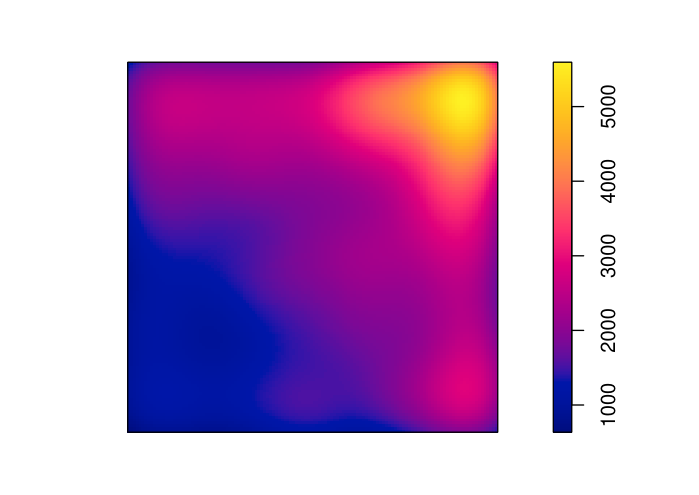
We also considered a two-dimensional Poisson process with intensity for . The outcomes of the algorithm, log-Gaussian Cox processes (LGCP) and kernel smoothing are illustrated in Figures 19-20 and Tables 30-32. The results demonstrate that the proposed algorithm performs well in this setting, is competitive with the kernel method, and spatial log-Gaussian Cox processes. In this scenario, the hyperparameter has been set equal to 1. In this scenario, the hyperparameter has been set equal to 1. The convergence criteria indicate convergence of the simulated chains (see also Section J).


| Inference with spatial log-Gaussian Cox processes | ||
| grid | AAE | RISE |
| 195 | 263 | |
| 182 | 245 | |
| Proposed Algorithm | ||||
|---|---|---|---|---|
| Number of trees | AAE for Posterior Mean | AAE for Posterior Median | RISE for Posterior Mean | RISE for Posterior Median |
| 8 | 177.44 | 175.62 | 255.23 | 258.88 |
| 10 | 176.52 | 174.02 | 253.14 | 255.92 |
| 15 | 177.48 | 172.62 | 254.22 | 251.96 |
| Kernel Smoothing | ||
|---|---|---|
| Bandwidth (sigma) | AAE | RISE |
| 0.03 | 360.11 | 463.1 |
| 0.04 | 277.89 | 353.82 |
| 0.087 (LCV) | 167.74 | 227.85 |
| 0.095 | 166.51 | 230.27 |
G.3 Inhomogeneous five dimensional Poisson Process with Gaussian intensity
Our next example is a five dimensional Poisson process with intensity for and the generated process via thinning consists of 343 points. The statistics are presented in Tables 33 and 34 for our algorithm and kernel smoothing, respectively. We have checked that the Gelman-Rubin criterion indicates convergence of chains.
| Proposed Algorithm | ||||
|---|---|---|---|---|
| Number of trees | AAE for Mean | AAE for Median | RISE for Mean | RISE for Median |
| 8 | 65.6 | 66.7 | 104.2 | 106.2 |
| 10 | 66.94 | 67 | 106.09 | 106.36 |
| Kernel Smoothing | ||
|---|---|---|
| AAE | RISE | |
| 0.03 | 631.1 | 5060.9 |
| 0.06 | 409.6 | 825.1 |
| 0.08 | 287.8 | 419.8 |
| 0.1 | 213.5 | 295.6 |
| 0.15 (LCV) | 181.2 | 278.5 |
| 0.3 | 258.4 | 363 |
| 0.5 | 311.2 | 409.7 |
Appendix H One dimensional Poisson Process with stepwise intensity
H.1 5 Trees
We run 3 parallel chains each for 200000 iterations keeping every 100th sample.
H.2 7 Trees
We run 3 parallel chains each for 200000 iterations keeping every 100th sample.
Appendix I One dimensional Poisson Process with with continuously varying intensity
I.1 5 Trees
We run 3 parallel chains each for 100000 iterations keeping every 50th sample.

I.2 10 Trees
We run 3 parallel chains each for 100000 iterations keeping every 50th sample.


Appendix J Inhomogeneous two-dimensional Poisson Process with Gaussian intensity
J.1 8 Trees
We run 3 parallel chains each for 200000 iterations keeping every 100th sample.

J.2 10 Trees
We run 3 parallel chains each for 200000 iterations keeping every 100th sample.

Appendix K Two dimensional Poisson process with stepwise intensity function
K.1 4 Trees
We run 3 parallel chains each for 100000 iterations keeping every 50th sample.
Appendix L Coal Data
L.1 8 Trees
We run 3 parallel chains each for 200000 iterations keeping every 100th sample.
L.2 10 Trees
We run 3 parallel chains each for 200000 iterations keeping every 100th sample.
Appendix M Earthquakes Data
M.1 10 Trees
We run 3 parallel chains each for 100000 iterations keeping every 50th sample.
Appendix N Mapples
N.1 5Trees
We run 3 parallel chains each for 300000 iterations keeping every 150th sample.
N.2 10 Trees
We run 3 parallel chains each for 300000 iterations keeping every 150th sample.
Appendix O Redwood
O.1 5 Trees
We run 3 parallel chains each for 300000 iterations keeping every 150th sample.

O.2 10 Trees
We run 3 parallel chains each for 300000 iterations keeping every 150th sample.
