Bayesian Predictive Beamforming for Vehicular Networks: A Low-overhead Joint Radar-Communication ApproachThanks: W. Yuan, J. Yuan, and D. W. K. Ng are with the School of Electrical Engineering and Telecommunications, University of New South Wales, Sydney, NSW 2052, Australia (e-mail: weijie.yuan@unsw.edu.au, j.yuan@unsw.edu.au, w.k.ng@unsw.edu.au).Thanks: F. Liu and C. Masouros are with the Department of Electronic and Electrical Engineering, University College London, London, WC1E 7JE, UK (e-mail: fan.liu@ucl.ac.uk, chris.masouros@ieee.org).Thanks: N. González-Prelcic is with the Department of Electrical and Computer Engineering, The University of Texas at Austin, Austin, TX 78712-1687, USA, and also with the Signal Theory and Communications Department, University of Vigo, 36310 Vigo, Spain (e-mail: ngprelcic@utexas.edu).
Abstract
The development of dual-functional radar-communication (DFRC) systems, where vehicle localization and tracking can be combined with vehicular communication, will lead to more efficient future vehicular networks. In this paper, we develop a predictive beamforming scheme in the context of DFRC systems. We consider a system model where the road-side units estimates and predicts the motion parameters of vehicles based on the echoes of the DFRC signal. Compared to the conventional feedback-based beam tracking approaches, the proposed method can reduce the signaling overhead and improve the accuracy. To accurately estimate the motion parameters of vehicles in real-time, we propose a novel message passing algorithm based on factor graph, which yields near optimal solution to the maximum a posteriori estimation. The beamformers are then designed based on the predicted angles for establishing the communication links. With the employment of appropriate approximations, all messages on the factor graph can be derived in a closed-form, thus reduce the complexity. Simulation results show that the proposed DFRC based beamforming scheme is superior to the feedback-based approach in terms of both estimation and communication performance. Moreover, the proposed message passing algorithm achieves a similar performance of the high-complexity particle-based methods.
Index Terms:
Dual-functional radar-communication, beam tracking, factor graph, vehicular networks.I Introduction
Connectivity and automation are revolutionizing the automotive industry. These technologies are enabling innovations that will transform vehicles into platforms for drivers and passengers that will provide services beyond transportation[1, 2]In the era of the fifth-generation (5G) communication, vehicle-to-everything (V2X) communication is expected to play an important role to support promising applications including automated vehicles, traffic management, and social driving [3]. To fulfill the stringent quality of service (QoS) requirement in 5G, the V2X network is required to support low latency information transmission in high-mobility environments[4]. In addition to the wireless communication, the environment sensing capability is also of great importance in vehicular networks. Since its birth, radar systems have been already deployed worldwide to address several military and civilian applications such as obstacle detection, environment reconstruction, as well as remote sensing [5]. In the future V2X systems, due to the time-varying nature of the network topology and the surrounding environments, radar-type technologies are envisioned as a promising candidate for detecting and tracking cars, pedestrians, road lanes, and obstacles in real-time [6].
Traditionally, radar and communication systems exploit separate spectrum resources and thus rarely interfere with each other. However, this approach becomes challenging, or even infeasible, as the communities developing both types of systems are seeking more resources. As a result, for V2X applications, where both radar and communication functionalities are desirable, mutual interference is unavoidable in overlapped frequency bands. A straightforward solution is to allocate two systems with separated portions of frequency spectrum to eliminate any possible interference, yet, resulting in a severe degradation of the spectral efficiency. Departing from this naive approach, a recent stream of research focuses on the design of joint systems that perform both radar sensing and communication functionalities with a single transmission. That is the dual-functional radar communication (DFRC) technique, which is capable of significantly reducing the hardware cost while increasing the overall system throughput[7].
Early contributions of DFRC designs focused on the employment of orthogonal frequency division multiplexing (OFDM) technique[8]. OFDM offers several advantages for wireless communication systems, such as resilience to multi-path fading, simple time and frame synchronization, and low-complexity equalization. From the radar sensing perspective, OFDM-like radar signals decouple the range and Doppler estimators in contrast to conventional radar systems, which provides a better target estimation performance [9]. Thus, OFDM has been regarded a promising candidate for implementing DFRC systems [10, 11]. To satisfy the requirement of communication with multiple users, DFRC systems based on the multiple-input multiple-output (MIMO) technology have been proposed in recent work. In MIMO radar, the waveforms radiated by each antenna element are orthogonal, thus the interference can be avoided and more degrees of freedom are available for DFRC waveform design. Pioneered by [12], a MIMO DFRC approach is proposed to detect target using the mainlobe of the spatial beampattern, while transmitting useful information by varying the sidelobe power. Later on, more advanced DFRC approaches were studied under various conditions and constraints, such as Non Line-of-Sight (NLoS) channels [13], multi-user interference and peak-to-average-power ratio (PAPR)-constrained transmission [14]. However, the aforementioned works focus on the sub-6G Hz frequency band and cannot support Gbps data rate as required by V2X communication systems.
To overcome the above challenges, the large bandwidth available in the millimeter wave (mmWave) spectrum is considered as a key enabler for DFRC systems, which can significantly improve both the data rate for communication and the range resolution for radar. In particular, by leveraging the massive MIMO technology, mmWave systems are able to exploit efficient spatial processing methods such as beamforming and spatial multiplexing at the transmitter and/ or receiver sides [15, 16]. Aiming for designing DFRC transceivers at the mmWave band, the authors of [17] designed an adaptive DFRC waveform that meets the Pareto optimal bound. Then a novel framework based on hybrid analog-digital beamforming techniques was developed in [7]. However, [7] did not take the high-mobility environments into account and their results are thus not suitable for V2X applications. Relying on the large-scale antenna array, the pencil-like spatial beams can be generated by the transmitter focusing the radiation power on the intended directions, which compensates for the high path-loss of the mmWave signals. To establish a reliable communication link, it is essential to align the transmit and receive beams between the vehicles and the associated road-side unit (RSU) [18]. Conventionally, the RSU periodically scans the angular interval of interest and pairs the transmit and receive beams with the strongest channel gain. However, for the vehicular applications with dynamic network topology and environments, the beam pairing has to be done frequently, leading to exceedingly high communication cost.
To cope with the high-mobility constraint imposed on the V2X scenarios, several works considered the fast beam tracking problem from the communication perspective[19, 20].In [20], the RSU first sends a communication signal containing pilots to the vehicles. Then the vehicles decode the information and estimate the relative angles with respect to the RSU, which are then fedback to the RSU for beam steering to the intended direction. To reduce the latency for beam alignment, the RSU can have a further prediction of the relative angles in the next time slot. Then the RSU can adopt their beamformers ahead for establishing the communication link in the following time instant. Some recent works utilized the classic Extended Kalman filtering (EKF) based on the state evolution of vehicles to predict the angles [21]. Except for the angular parameters, it is important to track the variation of other kinetic motion parameters of vehicles such as speed and range to fulfill the requirements of intelligent traffic applications. To achieve highly accurate estimation result, the number of pilots for EKF beam tracking should be sufficiently large, leading to high communication signaling overhead. Some radar aided beam alignment method were proposed in [22, 23],where the radar signal operates in a different frequency band, which however leads to increased spectral consumption. For these reasons, we develop a DFRC-based scheme for tracking the beam direction as well as the motion parameters in vehicular networks.
In this paper, we propose a novel DFRC-based predictive beamforming scheme for vehicle-to-infrastructure (V2I) scenarios that has a very low signaling overhead. To elaborate, the RSU sends DFRC signals containing information to the vehicles via downlink transmission. After receiving the DFRC signals, the vehicles perform detection followed by decoding to obtain the information. Meanwhile, the echoes reflected by the vehicles are acquired by the RSU via radar sensing techniques to estimate the beam directions as well as other motion parameters of the vehicles. With the help of the radar system, feedbacks from the vehicles to the RSU can be avoided. Compared to some feedback-based schemes that exploits a limited number of pilots for beam tracking, e.g. [21], the proposed DFRC-based scheme utilizes the whole downlink block both as communication data symbols and sensing pilots. Therefore the signaling overhead solely for beam alignment is as low as , which undoubtedly increases the spectral efficiency. Accordingly, uplink resources can be fully exploited for transmitting data rather than carrying feedback information. Different from the feedback-based methods, the “prediction” is done at the RSU, and the predicted angular parameters are contained into the DFRC signals sent to the vehicles. To fully realize the DFRC-based predictive beamforming, we formulate the beam tracking problem as a Bayes inference. In contrast to our previous work [24], we commence from the optimal estimation perspective and propose a factor graph and message passing-based algorithm to estimate and predict the motion parameters of vehicles at each time slot. Compared to the EKF method in [24], the proposed approach is expected to achieve a better estimation performance. Note that the product factor node and the nonlinear functions concerning the angular parameters complicate the considered problem making the standard message passing algorithm inapplicable to provide any closed-form solutions. In general, particle filtering (PF) can be used for accurately approximating the non-closed form messages. However, the employment of a large number of particles results in high complexity. To strike a balance between the complexity and performance, we propose a modified mean field (MF) message passing algorithm and apply second-order Taylor expansion to linearize the inverse trigonometry functions. As a result, all messages are derived in a closed-form, leading to a low level of computational complexity. In a nutshell, our contributions are summarized as follows:
- •
We propose a DFRC based predictive beamforming scheme for vehicular networks, achieving a better estimation performance and higher spectral efficiency than that of conventional feedback-based schemes. We consider a prediction of the angles for formulating the beamformers in order to reduce the latency.
- •
We introduce a specifically tailored factor graph-based framework and a message passing algorithm to accurately track and predict the motion parameters of vehicles.
- •
We exploit the MF message passing and Taylor expansion approaches for deriving closed form messages on factor graph, providing a low-complexity and high-accuracy estimation result.
Simulation results show that our proposed algorithm achieves a similar performance of the PF-based method but with only a considerably lower computational overhead. Moreover, compared to the communication-only feedback scheme [21], the proposed algorithm achieves better tracking performance and higher achievable rate.
The remainder of this paper is organized as follows. We introduce the DFRC signal model and the kinematic model of vehicles in Section II. Section III constructs the factor graph based on the probabilistic model of the considered system. In Section IV, the proposed message passing algorithm for beam tracking and motion parameter estimation is described. Then the simulation results are shown and discussed in Section V. Finally, our conclusions are drawn in Section VI.
Notations: We use a boldface letter to denote a vector. The superscripts , and denote the transpose, the conjugate, the inverse and the Hermitian operations, respectively; denotes the Gaussian distribution of real variable having mean of and variance of ; denotes all variables in set except ; represents the expectation operator; denotes the operator to obtain the variance of a random variable; denotes a complex space of dimensional ; and denote the real part and imaginary part of a complex variable; represents the modulus of a complex number; represents both sides of the equation are multiplicatively connected to a constant; denotes the error function; denotes all variables in except .
II System Model
Throughout this paper, we consider a vehicular network with one RSU supporting vehicles, as depicted in Fig. 1. The RSU operates at mmWave band equipped with a massive MIMO uniform linear array (ULA) which has transmit antennas and a separate array of receive antennas. This allows the RSU to receive the vehicle echoes for tracking while ensuring uninterrupted downlink transmission. Each one of the vehicles is assumed to have an -antenna ULA mounted on both sides of its body. The vehicles move along a one-lane straight road parallel to the RSU array11 1 For convenience of exposition, the vehicles are modeled as point targets following standard assumption in the literature [25]. The extension to a non-parallel case is straightforward since the angle between the road and the RSU array is fixed and known to the RSU and can be easily calibrated.. For brevity, we assume that the signals transmit through line-of-sight (LoS) channels, a further extension to non line-of-sight channels will be designated to the future works.

Without loss of generality, we denote the range, the angle, and the speed of the th vehicle relative to the RSU’s array by , , and , respectively. Provided that the vehicle is moving along the direction parallel with the ULA, the angle of the RSU relative to the th vehicle can also be defined as . We further denote the time duration between two radar epochs by . Following commonly adopted assumptions[21], we assume that the required parameters for vehicle do not change in a relatively short time duration. Then the motion parameters of vehicle at the th time instant are denoted by , , and .
II-A Signal Model
At the th instant, the RSU sends a -dimensional multi-beam direction-finding DFRC signal to the vehicles concurrently, denoted by with a complex signal for vehicle . The signal is transmitted over antennas of the RSU, formulating as
| (1) |
where is the transmit beamforming matrix. In general, the beamforming matrix is designed relying on the predicted angle. Assuming that we have a prediction of angle for all vehicles , defined by , the beamforming vector for the th vehicle is the th column of that can be written as
| (2) |
where denotes the signal power, with is the transmit steering vector and is the predicted angle at time . By using the beamforming matrix , each beam is steered towards the predicted angle of the targeted vehicle. The transmitted signal is reflected by all the vehicles and the received echo can be formulated as
| (3) |
where denotes the multi-antenna array gain, , , and denote the reflection coefficient, the Doppler, and the delay of the th vehicle at time , respectively, and is the receive steering vector with 22 2 It should be noted that we are considering a fully digital massive MIMO architecture, where the echo signal (3) is received by the RSU without analog combination.. The term is assumed to be a complex additive white Gaussian noise with zero mean.
Remark 1: The echoes may arrive at the RSU during the transmission of the DFRC signal, in which case the transmitted signal would inevitably generate self-interference to the reception. To address this issue, we employ separate transmit and receive antenna arrays at the RSU, with strong RF isolation combined with highly directive elevation beamforming. Then, the self-interference can be cancelled out via exploiting classic RF full-duplex structure [26], where the residual interference is small enough to be incorporated into the noise term. For notational convenience and to avoid alleviating from the focus of this paper, we will not discuss this topic in detail and designate this as our future work.
Given the relative range of vehicle and the RSU, i.e., , the reflection coefficient can be modeled as
| (4) |
where represents the complex radar cross-section (RCS)[5].
According to [27], the following result generally holds for ULA in a massive MIMO scenario:
| (5) |
This result indicates that the steering vectors related to two different vehicles are asymptotically orthogonal in massive MIMO systems [21]. Therefore, we assume that there is only negligible inter-beam interference and the RSU can identify the echoes from different vehicles. The reflected echo for the th vehicle can then be expressed as
| (6) |
where . In the following section, we will introduce the measurement model adopted at the RSU.
II-B Observation Model
By performing radar matched filtering on (II-A) with a delayed and Doppler-shifted version of , we obtain the estimates of delay and Doppler , which are related to range and speed , respectively. Considering Gaussian observation noise, the measurement model for the motion parameters and are given by
| (7) | ||||
| (8) |
respectively, where and represent the carrier frequency and signal propagation speed, noise terms and obey Gaussian distributions and , respectively.
Remark 2: By only exploiting the observation within a single time-slot, the speed estimation of a vehicle at the RSU is challenging, since the resultant Doppler phase shift is not significant [28]. To tackle this issue, one may estimate the vehicle’s velocity given a Doppler shift accumulated within multiple time-slots.
Having the estimates of delay and Doppler, we have the received signal samples for and based on the filtered signal, given by
| (9) |
where the term denotes the noise samples at different receive antennas. Without loss of generality, we model , . Remark that after matched filtering, we achieve a signal-to-noise ratio (SNR) gain , which is typically identical to the energy of signal . Vector in (9) denotes the transmit beamformer for vehicle based on the predicted angle at time instant . After straightforward manipulations, we arrive at the following measurement model
| (14) |
where . Next, we consider the state evolution model of the motion parameters of vehicles.
II-C State Evolution Model
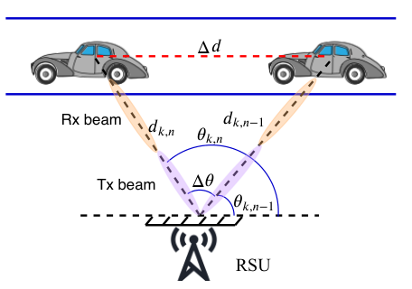
We aim for obtaining the motion parameters of all vehicles in the coverage area of the RSU. Based on the previous states and the moving patterns of the vehicles, we can determine the state evolution models for the vehicles, as shown in Fig. 2. Relying on the geometric relationship of the motion parameters at time instant and as shown in Fig. 2, we have the following kinematic equations as
The above two equations show how the motion parameters of vehicle evolve with time. For brevity, we define and . Obviously, solving the above nonlinear equations to construct the evolution model is challenging. As a compromise approach, we propose to find a tractable approximation of (II-C). Since in general, the variation of vehicle’s position is relatively small within a short period , we can use the approximation . Based on this, the first equation of (II-C) can be written as
| (17) |
By considering the fact that in time duration , is further expressed as
| (18) |
For the range variation in two continuous time slots, we can rewrite the second equation of (II-C) as
| (19) |
Then, by exploiting the fact that , (19) can be simplified to
| (20) |
Comparing to the range , the variation is negligible, therefore the term can be omitted and is given by
| (21) |
Furthermore, using the reflection coefficient model (4), we have
| (22) |
Finally, we assume that the speed of the vehicle is approximately a constant, i.e.,
| (23) |
Having (18)-(23), we summarize the state evolution models for , range , speed , and coefficient in the following
| (24) | ||||
| (25) | ||||
| (26) | ||||
| (27) |
where the transition noise , , , and obey zero mean Gaussian distributions , , , and , respectively. Note that the state evolution of , , and also depend on other variables. For simplicity, we adopt the estimates at time instant , i.e., , , and to replace the corresponding terms in (24)-(27), such that the evolution of the motion parameters only depends on their own previous states.
II-D Communication Model
To receive the signal sent by the RSU, vehicle adopts a receive beamformer and the received signal is formulated as
| (28) |
where is the array gain between the RSU and the vehicle, is the channel pathloss coefficient, is the Gaussian noise term, and denotes the receive steering vector of vehicle , which has a similar definition as . The beamformer is designed based on the predicted angle of vehicle relative to the RSU at time instant , i.e., . The prediction of the angle at time is done at the RSU based on the estimate at time , which is contained in the DFRC signal at time to the th vehicle. Assuming that the original transmitted signal from the RSU has unit power, then the SNR of the received signal is given by
| (29) |
where is the power spectral density (PSD) of the additive white Gaussin noise. Substituting the expression of into (29) yields
| (30) |
Based on the SNR corresponding to the th vehicle, the achievable sum-rate of all vehicles at time is expressed as
| (31) |
It can be observed that the achievable sum-rate relies on the transmit and receive beamformers. When the angle is perfectly predicted, i.e., , and , the received SNR is maximized, given by
| (32) |
and we have the maximum achievable sum-rate. For the channel coefficient , it can be simply estimated based on the range parameter .
For clarity, we define vectors , , and as the received signals, observed delays and Dopplers of vehicle until time instant , respectively. Furthermore, the unknown parameters corresponding to vehicle can also be rewritten in vector form as , , and , respectively. As the echo signals reflected by different vehicles can be identified unambiguously, in what follows, we will omit the vehicle index ‘’ for brevity. Note that the proposed algorithm is applicable for any vehicles in the RSU’s coverage area. In the above, we have expressed the radar signal as well as the communication model. In the next section, we will formulate a factor graph model to infer the variables representing the motion parameters of vehicles.
III Factor Graph Model
Our goal is to estimate the unknown range , speed , angle , and path loss given the state evolution model and the observation model. From the Bayesian perspective, this is equivalent to inferring the variables from the observations through an estimator, i.e., the maximum a posteriori (MAP) estimator,
| (33) |
where denotes the joint a posteriori distribution. Nevertheless, solving (33) involves a multi-dimensional search, leading to an exponentially increased complexity. As a result, there is a need for a low-complexity estimation approach. To this end, we aim for finding a suboptimal solution that the maximization is performed based on the marginal a posteriori of a variable of interest , formulated as . Generally, the marginal distribution can be obtained through direct marginalization of the joint distribution, i.e.,
| (34) |
However, direct marginalization requires a prohibitively high complexity due to the multi-dimensional integrations involved in (34). In what follows, we will resort to the factor graph framework to obtain the marginals of unknown variables by leveraging the conditional independency between variables.
According to Bayes Theorem, the joint distribution is rewritten as
| (35) |
where and are the likelihood function and the joint a priori distribution, respectively. Let us consider the a priori distribution first. Based on the state transition function in (24)-(27), the joint a priori distribution can be factorized as
| (36) |
with the transition probabilities
| (37) | ||||
| (38) | ||||
| (39) | ||||
| (40) |
where The initial vehicle parameters at time instant are obtained by employing an omnidirectional probing waveform sent from the RSU. Based on the received echoes, the RSU is able to infer the parameters , , and of a vehicle entering the coverage area of RSU. Without loss of generality, we model the initial distributions of , , and as Gaussian distributions , , , and .
For the joint likelihood function, since the received signals, observed delays and Dopplers are irrelevant given the variables, we can express the joint likelihood function as
| (41) |
Considering that the Gaussian noise terms are independent for different time instants , therefore can be factorized as
| (42) |
where and . Recalling the model (II-B), the received signal at the th receive antenna consists of components, which makes the inference problem very difficult. Hence we introduce an auxiliary variable satisfying and . Based on the auxiliary variables, is given by
| (43) |
Following (35)-(III), we have the factorization of the joint a posteriori distribution and can represent it by a factor graph, as shown in Fig. 3, where each square represents an factor vertex and each circle denotes a variable vertex. In Fig. 3, the blue solid line boxed area and red dashed line boxed area correspond to the state evolution model and observation model, respectively. The shorthand notations , , , and denote the state transition probabilities , , , and , respectively. The factor vertices , , and denote the likelihood functions corresponding to the observations , and .
Having the factor graph, message passing algorithm can be implemented to efficiently compute the “beliefs” (approximate marginals) of unknown variables, which will be elaborated in the following section.
IV The Proposed Message Passing Approach
This section presents the proposed message passing algorithm for predicting and tracking the beam. There are two kinds of messages, i.e., the message from the factor vertex to the variable vertex and vice versa. For notational convenience, we use to denote the message from the factor vertex to the variable vertex and to denote the message from to factor .
IV-A Conventional Message Passing Algorithm
The conventional message passing algorithm, also known as belief propagation (BP) has defined the following message updating rules,
| (44) | ||||
| (45) |
where denotes the set of variables in function and denotes the set of factor vertices connected to . Having obtained all messages from to variable vertex , the belief (marginal) of variable is then given by
| (46) |
IV-B Vehicle State Prediction
As discussed in Section II, the RSU and the vehicles design the receive beamformers based on the predicted angles. With the estimates of the motion parameters at time , the RSU can predict angle via the state evolution model. Furthermore, the RSU can perform a prediction of the angle at time based on the information obtained at the th time instant. In this way, the information of the predicted angle is contained in the DFRC signal sent to the vehicles. After receiving the angle information, the vehicles can formulate the receive beamformer at the th instant using the predicted angles for in formation reception at time . If the prediction is sufficiently accurate, the transmit beams of RSU and the receive beams of vehicles are aligned, which leads to a better communication performance.
We commence our discussions with the messages in the state evolution part. Provided that the belief of has been obtained in Gaussian form as , the message is calculated according to (44), given by
| (47) |
It can be observed that the above message subjects to Gaussian distribution, which is characterized by the mean and variance . Therefore, we use the corresponding mean and variance to simplify the message derivations.
In a similar way, we can derive the messages , , and related to the vehicle predication based on the transition probabilities (38)-(40), expressing as
It can be observed that the means and variances in (IV-B) are updated based on the marginal mean and variance in the previous time instant and the state evolution model. Based on the Gaussian form message , we have the predicted angle at the th epoch as
| (54) |
which is used for designing the beamformer at the RSU.
In addition, to realize the predictive beamforming at all vehicles, the RSU performs a further prediction of the relative angle at time based on the estimate as well as the predicted motion parameters and , given by
| (55) |
The uncertainty of the angle is given by . The predicted angle is then sent to the vehicles for receive beam steering at time .
IV-C Vehicle State Tracking
At the th time instant, the vehicles receive the data information as well as the predicted angles for time . Then the vehicles can decode the information and formulate their beamformers to receive the signals at the th time instant. On the other hand, the RSU receives the echoes reflected by the vehicles. Based on the observations, the RSU is able to refine the estimates of the motion parameters at time . Then following the process in the above subsection, the RSU can predict the angles for the th and th time instants. In the following, we will discuss the messages calculations related to the observations.
IV-C1 Messages related to
The message is identical to the likelihood function since depends solely on . After straightforward manipulations, we write as
| (56) |
Then the belief of at time instant can be obtained as33 3 Note that the considered system is causal, therefore the motion parameters of vehicles depend only on the past states. The messages only forward along the time direction.
| (57) |
with the mean and variance being
| (58) | ||||
| (59) |
Since is a Gaussian distribution, the estimate of range is . The estimate is used for modeling the state evolution function (24). Also, the obtained belief is passed to factor vertex for calculating .
IV-C2 Messages related to
Then, we focus on the message updating concerning the speed variable. Note that (8) involves a nonlinear cosine function, calculating the message can not provide a closed-form expression. To tackle this problem, we reconstruct the factor node by introducing a factor vertex representing the cosine function and a variable vertex denoting the cosine of an angle, as illustrated in Fig. 4.
Provided the message obeys , we can now determine the message as
| (60) |
Although we derive a closed form solution for the integration problem, it is seen that the variable appears in both sides of the fraction bar, which indicates that we can not write the message in a Gaussian form. Hence we resort to the MF message passing algorithm, in which the message is defined as
| (61) |
Following (61), we can derive the Gaussian message , whose mean and variance are
| (62) | |||
| (63) |
respectively. Similarly, the mean and variance of are given by
| (64) | |||
| (65) |
respectively, where and are identical to and , respectively. The belief of can be obtained with message and and the estimate is used for predicating the parameters in the th epoch.
Next we move our focus to the nonlinear cosine function that maps the angle to a real number . According to the characteristic function [29], the expectation of given is . It is well known that , hence we have while . Considering the message , we can obtain parameters and as
| (66) | ||||
| (67) |
For message , the function turns to be an inverse cosine function. To overcome this nonlinear issue, one can directly employ the particle filtering (PF) based method by representing the nonlinear distributions by particles. However, the huge computational cost violates the low-latency requirement of vehicular applications. As an alternative, we employ the second order Taylor expansion concerning the inverse cosine function as . Then based on the obtained parameter and , we derive the Gaussian message as
| (68) | ||||
| (69) |
The detailed expression of is not given here, which involves the sixth-order moment of . Please refer to the generalized Hermite polynomials for the expressions of higher order moments of .
IV-C3 Messages related to
Next, we will derive the messages related to the observations . Assuming that all messages from to are known with Gaussian distributions, it is readily to obtain the message using MF rules as
| (70) | ||||
| (71) |
where , and . The mean and represents the information of the observation at the th receive antenna contributed to the variable . Having in hand, the belief of can be obtained according to (46) with mean and variance
| (72) | ||||
| (73) |
Obviously, the update of and depend on the state evolution information from the previous time instant as well as the information from the receive antennas. Consequently, the message from to a factor vertex is simply derived by
| (74) | ||||
| (75) |
Provided the Gaussian message , the message is computed as,
| (76) | ||||
| (77) |
Using (76) and (76), the information obtained from the observation is fed to the auxiliary variable and then to the angular parameter.
IV-C4 Messages related to
Finally, we aim for computing the messages related to the function , which involves the nonlinear function . Note that this part of factor graph has cycles, we have to implement the message passing algorithms for a few iterations[30]. As above, the mean and variance of given the Gaussian form input message can be calculated similar to (IV-C2) and (IV-C2), denoting by and . Employing the transformations of trigonometric functions and after some manipulations, we have the mean and variance for message , formulating as
| (78) | ||||
| (79) |
It is then straightforward to determine the message and as44 4 It may happen parial messages do not exist. In this circumstance, we cam simply set .
| (80) | ||||
| (81) |
The above two messages are still Gaussian since all messages on the right-hand-side of (80) and (81) are represented in Gaussian closed-form. Computing the backward message involves the inverse function of , which is not applicable to deliver Gaussian distributed variable . To this end, we reconstruct the function node , as shown in Fig. 5, on which the process for calculating is given in the following.
The real and imaginary parts of the mean as well as the variance of are passed to the inverse cosine (“acos”) and inverse sine (“asin”) functions, respectively. Then the mean and variance of message from the acos factor vertex to is calculated based on Taylor expansion similar to (IV-C2) and (69). The message related to asin function is calculated according to the second order Taylor expansion of inverse trigonometric function, given by . Then the mean of the message is expressed as
| (82) |
and the expression of variance having higher order moments is not given here. Consequently, the message is simply calculated by
| (83) |
In the end, the message is calculated in Gaussian form by implementing the Taylor expansion of inverse cosine function again, which has a similar form to that of (IV-C2) and (69). Having determined all messages form to , we arrive at the belief of ,
| (84) |
which is used for obtaining the message and for beam prediction at th time instant. The estimate of , given by , is used for constructing the state transition model.
In the above, we have solved the beam prediction and beam tracking problems based on the factor graph framework. With the help of the determined angular parameters, the RSU and the vehicle can maintain a reliable link for data transmission.
IV-D Beam Misalignment Analysis
Recalling that a vehicle can receive the predicted angle at the th time instant from the RSU at time instant , therefore can adjust the direction of its receive beamformer based on the prediction. As we have the mean value as well as the uncertainty , the beam-steering direction of the vehicle at the th time instant follows the Gaussian distribution . On the other hand, the beam prediction at the RSU is performed after the beam tracking process at time , as in (54).
In mmWave systems, the beamwidth is typically very narrow that beam misalignment may happen when the predicted angles of the RSU and at the vehicle differ from the actual angle. To analyze the probability of beam misalignment, we use to denote the beamwidth and beams are aligned only if the vehicle’s beam direction satisfying and the RSU’s beam direction satisfying , where denotes the actual angle of the vehicle relative to the RSU’s array and [31]. This is equivalent to calculating the probability of
| (85) | ||||
Given the distribution of , we have the cumulative distribution function (CDF) as
| (86) |
Similarly, we have the CDF for Gaussian distribution as
| (87) |
Consequently, the misalignment probability is calculated as
| (88) | ||||
Observed from the above analysis, the misalignment probability depends on the width of the beam, which motivates us to optimize the beamwidth in our future work to minimize the probability .
IV-E Computational Complexity and Signaling Overhead
Observe from Sec. IV-B and IV-C that the complexity of the proposed algorithm is dominated by the calculations of corresponding messages. It is worth to see that all messages can be written in a closed-form by employing appropriate approximations and message updating rules. Hence, the message calculations only involve trivial addition and multiplication operations, leading to a very low level of complexity. To elaborate, the order of complexity of the proposed algorithm can be given by . In contrast, the PF-based algorithm adopts particles to represent the nonlinear functions, which has the order of complexity . In general, should be sufficiently large to achieve a reasonably good estimation performance, and the complexity is significantly increased. As a commonly used scheme for beam tracking, the extended Kalman filtering (EFK) requires the matrix inversion, having a complexity order of cube of the matrix dimension, i.e., . Through this complexity comparison, we show the superiority of the proposed algorithm in the large scale vehicular networks. Concerning the signaling overhead, the feedback-based approach usually utilizes one or two pilot symbols for beam tracking. For the proposed DFRC-based beam tracking scheme, since the whole downlink block is used for transmitting data information, the signaling overhead much lower than the feedback-based scheme.
V Simulation Results

Let us consider a network with 4 vehicles moving on the road, as shown in Fig. 6. Without loss of generality, the coordinate of the RSU is set as and the initial positions of vehicles are , , , and , respectively. The RCS is set to , which is used for calculating the reflection coefficient via (4). The speeds of four vehicles at time instant are randomly generated from the uniform distribution m/s. The RSU and the vehicles are operating at a carrier frequency of GHz. The time slot duration is and the signal propagation speed is approximated as m/s. For brevity, we set both the radar noise variance and the noise PSD for communication to 1. For the observed delays and Dopplers at RSU, we use the standard deviations of s and kHz for all vehicles at different time slots. The state transition noises are set with standard deviations of m, m/s, , and . For the log-distance pathloss model, we assume a unit channel gain at the reference distance m. The maximum number of iterations for message passing algorithm is set to . All results are averaged from 1000 independent Monte Carlo simulations unless otherwise specified.

We first consider the tracking performance of the motion parameters of vehicles relying on the proposed approach. In Fig. 7, we show the tracking result of the range parameter in terms of root mean squared error (RMSE). The RMSE is averaged from the results obtained for all 4 vehicles. Four deployments with different number of transmit and receive antennas are illustrated. For all cases, it is interesting to see the curves first decreases and then increases with respect to the time index. This is because when the vehicles move towards the RSU, the reflection coefficient becomes larger, leading to a higher SNR gain. On the contrary, the SNR deceases when the vehicles are moving away. Moreover, employing a larger scale antenna array will introduce a higher array gain as well as more observations, therefore resulting in a better tracking performance. The averaged RMSE of angle estimation parameterized by different number of antennas is depicted in Fig. 8. Obviously, the RMSE curves for angle tracking have a similar trend as that in Fig. 7. It is also observed that the estimation of the angle is very accurate, at the error level of rad.

Next we compare the performance of the proposed approach and the classic feedback-based algorithm. For fair comparison purpose, we still employ the factor graph and message passing algorithm for the feedback-based scheme55 5 Existing feedback-based methods [21] rely on the EKF, which in general has a worse performance than message passing algorithm due to using first-order Taylor series expansion.. Note that in the feedback-based scheme, the pilots are contained in the downlink communication signal. Therefore, the reflection parameter in the observation model of (II-B) is replaced by channel gain , which is determined by estimating the range parameter . In contrast to the DFRC signal that the whole block can be used as the pilots, the feedback scheme can employ only 1 or 2 pilots, leading to a much smaller SNR gain after matched filtering. For simplicity, we equivalently multiply the noise variance by a constant for the feedback-based scheme. We compare the CDF of the estimation error of based on the proposed approach and the feedback scheme at the last time instant with antennas. The high-complexity PF-based message passing algorithm and the EKF method in [24] are utilized as a benchmark. It is observed that with significantly reduced complexity, the proposed parametric message passing method can attain the performance of the PF-based one, verifying the effectiveness of applying Taylor series expansion and MF message passing. Moreover, the proposed approach significantly outperforms the feedback-based scheme with 1 and 2 pilots due to the higher SNR gain.


Fig. 10 evaluates the angle estimation result using the proposed approach, the feedback scheme, and the EKF method in [24]. We illustrate the CDF versus the angle estimation error at the last time instant for 1000 trails. Two cases with 64 and 128 antennas are illustrated. We see that for both cases, the feedback scheme suffers from a remarkable performance loss due to limited matched-filtering gain. In contrast to the proposed approach, increasing the number of antennas for the feedback scheme will lead to performance degradation. This can be explained by the fact that a higher number of antennas provides a narrower beam, in which case using only 1 pilot is not sufficient to track the variation of the angular parameter. Moreover, the proposed algorithm outperforms the EKF method since EKF employs only the first-order Taylor expansion and neglect the higher-order information. Since the estimated angles are used for beamforming design, the tracking error of angles will result in the misalignment of the beams. As a consequence, the received SNR is reduced, leading to a lower achievable rate. In Fig. 11, we illustrate the CDF of the communication achievable rate of all time instants based on the proposed and the feedback-based methods at a SNR of 10 dB. For the proposed scheme, the achievable rate at different time instants are higher than 4 bps/Hz. While the achievable rate for the feedback-based scheme is much lower. This validates our discussions above that the large angle estimation error in the feedback-based approach degrades the achievable rate. Furthermore, the rate degradation becomes more significant for the feedback-based scheme in the case with 128 antennas, where the angle variation cannot be accurately tracked due to the narrow beamwidth. Figs. 10 and 11 show the superiority of employing DFRC signaling for reliable communication in vehicular networks.
Finally, we consider the misalignment probability with different widths of the beam. According to (85), it is expected a wider beam will result in a lower misalignment probability. In Fig. 12, we depict the beam misalignment probabilities of two kinds of vehicles, i.e. high-speed vehicle having a speed in the interval [18, 20] m/s and low-speed vehicle having a speed in the interval [5,7] m/s, versus the time instant. The beamwidth of is achieved by activating only 16 antennas in the 128-antenna array. First we can see the misalignment probability for low-speed vehicle is lower than that for the high-speed vehicle. This is due to that the faster vehicle causes more violent variation of the relative angle . In addition, we observe that the high-speed vehicle is more sensitive to the beamwidth than the low-speed one. The misalignment probability experiences a significant rise when we choose . This motivates us to further optimize the beamwidth for vehicles with different speeds in practical scenarios.

VI Conclusions
In this paper, we proposed a novel DFRC based beamforming scheme for vehicular networks, providing zero signaling overhead for beam tracking. We commence from a Bayesian perspective and construct the joint a posteriori distribution based on the echo signals received at the RSU and the state transition models of the vehicles. The joint distribution was further fully factorized and represented by a factor graph, then the message passing algorithm is utilized to estimate the unknown variables. A second order Taylor expansion was employed to approximate the nonlinear inverse trigonometric functions. Consequently, the messages on factor graph were determined in closed-form, providing a low complexity solution for the considered beam tracking problem. A two-step prediction of angles are further processed and sent to the vehicles via DFRC signals, which can reduce the latency for beam alignment. Simulation results demonstrate the effectiveness and superiority of the proposed approach compared to the conventional feedback-based scheme.
References
- [1] J. E. Siegel, D. C. Erb, and S. E. Sarma, “A survey of the connected vehicle landscape—architectures, enabling technologies, applications, and development areas,” IEEE Trans. Intell. Transport. Syst., vol. 19, no. 8, pp. 2391–2406, Aug. 2017.
- [2] N. Lu, N. Cheng, N. Zhang, X. Shen, and J. W. Mark, “Connected vehicles: Solutions and challenges,” IEEE Internet. Things J., vol. 1, no. 4, pp. 289–299, Sep. 2014.
- [3] S. Chen, J. Hu, Y. Shi, Y. Peng, J. Fang, R. Zhao, and L. Zhao, “Vehicle-to-everything (V2X) services supported by LTE-based systems and 5G,” IEEE Commun. Stand. Mag., vol. 1, no. 2, pp. 70–76, Jan. 2017.
- [4] X. Wang, S. Mao, and M. X. Gong, “An overview of 3GPP cellular vehicle-to-everything standards,” GetMobile: Mobile Comput. Commun., vol. 21, no. 3, pp. 19–25, Mar. 2017.
- [5] M. I. Skolnik, RADAR systems. McGraw-Hill, NY, 2001.
- [6] J. Dickmann, J. Klappstein, M. Hahn, N. Appenrodt, H.-L. Bloecher, K. Werber, and A. Sailer, “Automotive radar the key technology for autonomous driving: From detection and ranging to environmental understanding,” in Proc. IEEE Radar Conf. IEEE, 2016, pp. 1–6.
- [7] F. Liu, C. Masouros, A. Petropulu, H. Griffiths, and L. Hanzo, “Joint radar and communication design: Applications, state-of-the-art, and the road ahead,” IEEE Trans. Commun., In press, 2020.
- [8] S. Sen and A. Nehorai, “Adaptive OFDM radar for target detection in multipath scenarios,” IEEE Trans. Signal Process., vol. 59, no. 1, pp. 78–90, Jan. 2010.
- [9] C. Shi, F. Wang, M. Sellathurai, J. Zhou, and S. Salous, “Power minimization-based robust OFDM radar waveform design for radar and communication systems in coexistence,” IEEE Trans. Signal Process., vol. 66, no. 5, pp. 1316–1330, Mar. 2017.
- [10] C. Sturm and W. Wiesbeck, “Waveform design and signal processing aspects for fusion of wireless communications and radar sensing,” Proc. the IEEE, vol. 99, no. 7, pp. 1236–1259, Jul. 2011.
- [11] A. R. Chiriyath, B. Paul, and D. W. Bliss, “Radar-communications convergence: Coexistence, cooperation, and co-design,” IEEE Trans. Cog. Commun. Netw., vol. 3, no. 1, pp. 1–12, Jan. 2017.
- [12] P. Kumari, N. Gonzalez-Prelcic, and R. W. Heath, “Investigating the IEEE 802.11 ad standard for millimeter wave automotive radar,” in Proc. IEEE Veh Technol. Conf. IEEE, 2015, pp. 1–5.
- [13] F. Liu, C. Masouros, A. Li, H. Sun, and L. Hanzo, “MU-MIMO communications with MIMO radar: From co-existence to joint transmission,” IEEE Trans. Wireless Commun., vol. 17, no. 4, pp. 2755–2770, Apr. 2018.
- [14] F. Liu, L. Zhou, C. Masouros, A. Li, W. Luo, and A. Petropulu, “Toward dual-functional radar-communication systems: Optimal waveform design,” IEEE Trans. Signal Process., vol. 66, no. 16, pp. 4264–4279, Aug. 2018.
- [15] S. Sun, T. S. Rappaport, R. W. Heath, A. Nix, and S. Rangan, “MIMO for millimeter-wave wireless communications: Beamforming, spatial multiplexing, or both?” IEEE Commun. Mag., vol. 52, no. 12, pp. 110–121, Dec. 2014.
- [16] K. Venugopal, M. C. Valenti, and R. W. Heath, “Device-to-device millimeter wave communications: Interference, coverage, rate, and finite topologies,” IEEE Trans. Wireless Commun., vol. 15, no. 9, pp. 6175–6188, Sep. 2016.
- [17] P. Kumari, S. A. Vorobyov, and R. W. Heath, “Adaptive virtual waveform design for millimeter-wave joint communication-radar,” IEEE Trans. Signal Process., vol. 68, pp. 715–730, Jan. 2020.
- [18] S. Haghighatshoar and G. Caire, “The beam alignment problem in mmwave wireless networks,” in Proc. Asilomar Conf. IEEE, Jul. 2016, pp. 741–745.
- [19] V. Va, H. Vikalo, and R. W. Heath, “Beam tracking for mobile millimeter wave communication systems,” in Proc. IEEE Global Conf. Signal. Inf. Process. IEEE, 2016, pp. 743–747.
- [20] D. Zhang, A. Li, M. Shirvanimoghaddam, P. Cheng, Y. Li, and B. Vucetic, “Codebook-based training beam sequence design for millimeter-wave tracking systems,” IEEE Trans. Wireless Commun., vol. 18, no. 11, pp. 5333–5349, Nov. 2019.
- [21] S. Shaham, M. Ding, M. Kokshoorn, Z. Lin, S. Dang, and R. Abbas, “Fast channel estimation and beam tracking for millimeter wave vehicular communications,” IEEE Access, vol. 7, pp. 141 104–141 118, 2019.
- [22] N. González-Prelcic, R. Méndez-Rial, and R. W. Heath, “Radar aided beam alignment in mmwave V2I communications supporting antenna diversity,” in Prof. Inf. Theory Applic. Workshop. IEEE, Jun. 2016, pp. 1–7.
- [23] A. Ali, N. González-Prelcic, and A. Ghosh, “Millimeter wave V2I beam-training using base-station mounted radar,” in Proc. IEEE Radar Conf. IEEE, 2019, pp. 1–5.
- [24] F. Liu, W. Yuan, C. Masouros, and J. Yuan, “Radar-assisted predictive beamforming for vehicular links: Communication served by sensing,” arXiv preprint arXiv:2001.09306, 2020.
- [25] H. Wymeersch, G. Seco-Granados, G. Destino, D. Dardari, and F. Tufvesson, “5G mmwave positioning for vehicular networks,” IEEE Wireless Commun., vol. 24, no. 6, pp. 80–86, Jun. 2017.
- [26] J. Palacios, J. Rodriguez-Fernandez, and N. Gonzalez-Prelcic, “Hybrid precoding and combining for full-duplex millimeter wave communication,” in Proc. IEEE Global Commun. Conf. IEEE, 2019, pp. 1–6.
- [27] T. L. Marzetta, Fundamentals of massive MIMO. Cambridge University Press, 2016.
- [28] J. Eaves and E. Reedy, Principles of modern radar. Springer Science & Business Media, 2012.
- [29] A. Feuerverger, R. A. Mureika et al., “The empirical characteristic function and its applications,” The Annals Stat., vol. 5, no. 1, pp. 88–97, Jan. 1977.
- [30] A. T. Ihler, W. F. John III, and A. S. Willsky, “Loopy belief propagation: Convergence and effects of message errors,” J. Mach. Learn. Res., vol. 6, no. May, pp. 905–936, 2005.
- [31] J. Zhang, E. Björnson, M. Matthaiou, D. W. K. Ng, H. Yang, and D. J. Love, “Multiple antenna technologies for beyond 5G,” arXiv preprint arXiv:1910.00092, 2019.