跳到论文正文
W Papers独立论文阅读器 arXiv:2005.07587 论文正文 计算阅读时间 · 0%
引用这篇论文根据当前论文元数据生成,正式投稿前建议核对。


License: arXiv.org perpetual non-exclusive license
arXiv:2005.07587v2 [math.ST] 28 Feb 2021

Non-Sparse PCA in High Dimensions via Cone Projected Power Iteration

Yufei Yi Email: yy544@cmu.edu    Matey Neykov Email: mneykov@stat.cmu.edu
Department of Statistics and Data Science, Carnegie Mellon University
5000 Forbes Ave, Pittsburgh, PA 15213, U.S.A.
Abstract

In this paper, we propose a cone projected power iteration algorithm to recover the first principal eigenvector from a noisy positive semidefinite matrix. When the true principal eigenvector is assumed to belong to a convex cone, the proposed algorithm is fast and has a tractable error. Specifically, the method achieves polynomial time complexity for certain convex cones equipped with fast projection such as the monotone cone. It attains a small error when the noisy matrix has a small cone-restricted operator norm. We supplement the above results with a minimax lower bound of the error under the spiked covariance model. Our numerical experiments on simulated and real data, show that our method achieves shorter run time and smaller error in comparison to the ordinary power iteration and some sparse principal component analysis algorithms if the principal eigenvector is in a convex cone.

Keywords— Power iteration; Dimension reduction; Principal Component Analysis; Convex cone; Monotone cone.

1 Introduction

Principal component analysis was developed by Hotelling, 1933 after its origin by Pearson, 1901, and is widely used nowadays for dimension reduction. It works by replacing a set of pp variables with a smaller set of principal components which capture the maximal variance. A principal component is a linear combination of the pp covariates. The coefficients of such a linear combination depend on the principal eigenvectors of the population covariance matrix, which is often estimated by eigenvectors of the sample covariance matrix. Numerical methods to compute principal eigenvectors include the QR algorithm and power iteration (Watkins, 2004, Chapter 5).

The consistency of principal component analysis is thoroughly studied in the statistical literature. See for example Paul, 2007; Nadler et al., 2008; Bai and Silverstein, 2010; Fan and Wang, 2015. In low dimensions (p≪n)(p\ll n), the sample estimators consistently recover the population principal eigenvectors (Anderson, 2003). However in high dimensions (p≫n)(p\gg n), all methods fail to recover the population principal eigenvectors if there is no additional structure imposed. Johnstone and Lu, 2009 introduced the spiked covariance model and proved that the sample estimator would not be consistent if p/np/n is bounded away from zero. Wainwright, 2019 shows that the minimax risk for estimating the spiked eigenvector is lower bounded by a quantity related to p/np/n.

In this paper, we study the problem of estimating the principal eigenvector of a positive semi-definite matrix in high dimensions, given that this vector belongs to a known convex cone. We view this setup as an alternative to the commonly used sparse PCA. Of course there are many ready-to-use methods available for sparse PCA, but we recognize that the first principal eigenvector might not always be sparse. The idea of considering general convex cone constraints is inspired by the fact that the set of ss-sparse vectors forms a cone (albeit a non-convex one). We stick with the convex cone constraint for two reasons: there are adequate results in convex analysis literature to support the analysis of our algorithm, and the set of convex cones is general enough to cover some useful cases. One example is the non-negative orthant cone, which arises in neural signal processing (Pavlov et al., 2007; Quiroga and Panzeri, 2009), computer vision (Lee and Seung, 1999; Arora et al., 2016), and gene expression (Lazzeroni and Owen, 2002). Another example would be the monotone cone. In time series forecasting, where often times more recent observations are more important, imposing monotonicity constraints makes intuitive sense. In addition due to the nature of the monotone cone, vectors can be estimated with high precision even in very high-dimensional settings.

On the algorithmic side, we propose a cone projected power iteration to estimate the first principal eigenvector. This is inspired by the work of Yuan and Zhang, 2013, where the authors proposed a truncated power iteration to find the principal eigenvector assuming it is sparse. The truncated power iteration, may be effectively thought of as a projected power iteration over the cone formed by ss-sparse vectors. It is thus natural to investigate whether the same approach carries over to the distinct setting of a convex cone constraint. A bulk of the effort in our work is dedicated to making this precise. On the analytical side, we derive the time complexity of the proposed cone projected power iteration algorithm, and provide an upper bound and a lower bound of its estimation error. Some numerical experiments are implemented to address the usefulness of the cone projected power iteration algorithm.

1.1 Related Work

With the failure of ordinary principal component analysis in high dimensions, researchers have started to impose additional structure on the eigenvectors. Such a structure is exploited by introducing constraints or penalties. The simplest and most studied structure is that of sparsity. Methods exploiting the sparsity structure are referred to as sparse principal component analysis. As to the origin, Cadima and Jolliffe, 1995 first proposed the idea to approximate a given principal component by using only a subset of features. The first computational technique –SCoTLASS– was established by Jolliffe et al., 2003, which maximizes the variance of a principal component under the ℓ1\ell_{1} constraint of eigenvector, inspired by LASSO (Tibshirani, 1996). Afterwards, Zou et al., 2006 proposed ElasticNet SPCA to regress a principal component on pp variables with elastic net constraint (Zou and Hastie, 2005) to get a sparse eigenvector. Witten et al., 2009 established the connections between SCoTLASS and ElasticNet SPCA. In the seminal work of d’Aspremont et al., 2005, the computation of the first sparse eigenvector is formed as approximating the covariance matrix by a rank-one spike matrix under Frobenius norm with constrains on the spike vector. Then it is relaxed to a semidefinite programming problem. Vu et al., 2013a generalized the work of d’Aspremont et al., 2005 to compute more than one sparse eigenvectors by incorporating Fantope in the constraint function. Besides methods based on the relaxation of the sparsity constraint, there is also a substantial literature on non-relaxed optimization techniques. Moghaddam et al., 2006 computed the non-zero elements of a sparse eigenvector by solving an unconstrained optimization on corresponding submatrices. The submatrices is selected by bi-directional greedy search. Johnstone and Lu, 2009 proposed a method which uses the coordinates with highest variance after wavelet transforms of the data. Years later, some new numerical methods came up, such as the work of Yuan and Zhang, 2013 which integrated the power iteration algorithm with truncation in each iteration, and Ma et al., 2013 which incorporated the QR algorithm with a thresholding step. Theoretical analysis of the convergence rate of sparse principal analysis can be found in Birnbaum et al., 2013; Cai et al., 2013; Vu et al., 2013b.

Despite the pervasive study of sparse constraints in principal component analysis, the study of methods with other constraints are scarce in the literature. Examples of non-sparse constraints include a subspace constraint (De Bie et al., 2004) and a non-negative orthant cone constraint (Montanari and Richard, 2015). In addition to the fact that those two types of constraints are special cases of convex cones, our work is quite different from theirs: Montanari and Richard, 2015 analyze the error rate of the non-negative approximate message-passing algorithm under the spiked covariance model, and De Bie et al., 2004 proposes a subspace constrained spectral clustering algorithm without providing error analysis. A recent work from Cai et al., 2020 gives statistical analysis of constrained PCA under the matrix denoising model and the spiked Wishart model under very general constraints. In the present paper we use a different loss function from theirs, and we do not assume any statistical model on the data when deriving the upper bound of estimation error. We also propose a practical iterative algorithm, whereas Cai et al., 2020 rely on a constrained optimization formulation which may not be easily implementable. Moreover, in order to apply the general lower bound of Cai et al., 2020, one needs to construct local packing sets at different resolutions manually and solve an identity equating the resolution of the packing to the square root of the log of its cardinality. This is quite distinct from our lower bounds, which are also developed under the spiked Wishart model, since we provide a universal lower bound on the packing set we pick (which is different from that of Cai et al., 2020). Furthermore, our lower bound cannot be derived from that of Cai et al., 2020 as our loss function is smaller than the one they consider.

In this work we consider the same type of constraint as the work of Deshpande et al., 2014 (i.e., convex cone constraints), but our setting is different from theirs. Deshpande et al., 2014 consider a spiked Gaussian Wigner model A=ν​x¯​x¯⊺+ZA=\nu\bar{x}\bar{x}^{\intercal}+Z, where ZZ is a symmetric Gaussian noise matrix (Perry et al., 2018, Definition 3.2). In contrast, in this paper we estimate the principal eigenvector x¯\bar{x} of any population covariance matrix A¯\bar{A} from a positive semidefinite observation A=A¯+EA=\bar{A}+E, where EE is a mean-zero noise matrix. Our main results are not tied to any distributional assumptions on the error matrix, i.e., we provide deterministic inequalities which control the estimation error (in an L2L_{2} sense) in terms of certain cone-restricted norms of the error matrix. We then use those general results to analyze the spiked covariance model where the upper and lower bounds we prove nearly match in some special cases of the convex cone constraint, while the work of Deshpande et al., 2014 did not provide clear connections between the upper and lower bounds. Notice also that spiked Gaussian Wigner model in Deshpande et al., 2014 clearly differs from the spiked covariance model. Besides the big difference in the settings, we will draw some further comparisons between our results and that of Deshpande et al., 2014: (i) our algorithm is cleaner and does not require a tunable hyper-parameter, (ii) our algorithm provably has a finite run-time guarantee, (iii) our upper bounds are strictly sharper than the ones exhibited by Deshpande et al., 2014, (iv) our main lower bound result is markedly different from the lower bound result of Deshpande et al., 2014 which lower bounds the minimax risk without an explicit dependence on the signal strength.

1.2 Organization

The remaining part of the paper is structured as follows. Section 2 provides some common notations, sets up problem formally and gives a result on the spiked covariance model with conic constraints. Section 3 discusses why cone constrained eigenvector estimation is hard to solve in general, and provides error rate guarantees for the so-called idealized estimator. Section 4 is dedicated to introducing the cone projected power iteration algorithm, which also includes the study of its time complexity, convergence, and upper bound of the error rate. Section 5 provides a lower bound over the convex cone constrained principal eigenvector estimation problem. We compare the obtained upper and lower bound under the spiked covariance model. Some example convex cones are studied to derive more informative upper and lower bound. Section 6 presents both simulated and real data experiments to support our theoretical findings. Finally, a brief discussion is provided in Section 7.

2 Notation and Preliminary

In this section we formalize the problem, we outline some notation and provide a result on the spiked covariance model with conic constraints.

2.1 Problem Formulation

In this paper we focus on the following concrete problem. Suppose A¯\bar{A} is a p×pp\times p positive semidefinite matrix with a first principal eigenvector x¯∈K\bar{x}\in K where K⊂ℝpK\subset\mathbb{R}^{p} is a known convex cone. Then x¯\bar{x} is the solution of

arg​maxu∈K​⋂𝕊p−1⁡u⊺​A¯​u.\displaystyle\argmax_{u\in K\bigcap\mathbb{S}^{p-1}}u^{\intercal}\bar{A}u. (1)

where 𝕊p−1\mathbb{S}^{p-1} is the unit sphere in ℝp\mathbb{R}^{p}. Instead of observing A¯\bar{A} we assume we get to observe a noisy matrix A=A¯+EA=\bar{A}+E, where EE is the stochastic noise. The problem of interest becomes to recover x¯\bar{x} from a noisy observation AA, with prior knowledge that x¯∈K\bar{x}\in K and assuming that the noisy matrix AA is positive semidefinite. For example, AA could be the sample covariance matrix of a data set, and A¯\bar{A} could be its population covariance matrix.

Let v^\hat{v} be the estimated principal eigenvector. The loss function we use is ‖v^−x¯‖2∧‖v^+x¯‖2\|\hat{v}-\bar{x}\|_{2}\wedge\|\hat{v}+\bar{x}\|_{2}, which is sign invariant and aligns with the signless nature of an eigenvector. In several places we will also use ‖v^−x¯‖2\|\hat{v}-\bar{x}\|_{2} if it is assumed or guaranteed that v^⊺​x¯≥0\hat{v}^{\intercal}\bar{x}\geq 0. In passing, we also remark that there are other popular loss functions studied in PCA literature such as the square of the sine of the angle 1−(v^⊺​x¯)21-(\hat{v}^{\intercal}\bar{x})^{2}, or the projector distance ‖v^​v^⊺−x¯​x¯⊺‖F\|\hat{v}\hat{v}^{\intercal}-\bar{x}\bar{x}^{\intercal}\|_{F}. It’s not hard to show that ‖v^​v^⊺−x¯​x¯⊺‖F2=2−2​(v^⊺​x¯)2\|\hat{v}\hat{v}^{\intercal}-\bar{x}\bar{x}^{\intercal}\|_{F}^{2}=2-2(\hat{v}^{\intercal}\bar{x})^{2}, and both of these loss functions are in general strictly larger than ‖v^−x¯‖22∧‖v^+x¯‖22=1−|v^⊺​x¯|\|\hat{v}-\bar{x}\|^{2}_{2}\wedge\|\hat{v}+\bar{x}\|^{2}_{2}=1-|\hat{v}^{\intercal}\bar{x}|. However, it is also clear that for values |v^⊺​x¯||\hat{v}^{\intercal}\bar{x}| close to 11, the loss functions are of the same order. The latter observation implies that any small enough upper bound on our loss function implies a corresponding upper bound on the sine of the angle and the projector distance loss functions.

2.2 Notation

We now outline some commonly used notation. Let λ,μ\lambda,\,\mu denote the largest and second largest eigenvalues of A¯\bar{A} and let ν:=λ−μ\nu:=\lambda-\mu be the first eigengap of A¯\bar{A}.

Given a cone C⊂ℝpC\subset\mathbb{R}^{p}, a cone-restricted operator norm of a p×pp\times p matrix EE is defined as

‖E‖C\displaystyle\|E\|_{C} =supx,y∈C​⋂𝕊p−1|x⊺​E​y|,\displaystyle=\sup\limits_{x,y\in C\bigcap\mathbb{S}^{p-1}}|x^{\intercal}Ey|,

Notice that ‖E‖C\|E\|_{C} constitutes a seminorm, and one trivially has ‖E‖C≤‖E‖o​p\|E\|_{C}\leq\|E\|_{op} where ‖E‖o​p\|E\|_{op} is the operator norm of EE. For completeness we mention that other forms of cone-restricted norms have also appeared in conic optimization literature (Amelunxen and Lotz, 2014, Section 1.2).

For a set T⊂ℝpT\subset\mathbb{R}^{p}, define the Gaussian complexity of TT as

w⁡(T)\displaystyle w(T) =𝔼​supt∈T⟨g,t⟩,where​g∼𝒩⁡(0,Ip),\displaystyle=\mathbb{E}\sup\limits_{t\in T}\,\,\langle g,t\rangle,\hskip 9.24994pt\text{where}\,\,g\sim\mathcal{N}(0,I_{p}),

which is the expectation of maximum magnitude of the canonical Gaussian process on TT. The Gaussian complexity of set TT can be upper bounded in terms of the metric entropy of TT via Dudley’s integral inequality (Vershynin, 2018, Theorem 8.1.10). Gaussian complexity is a basic geometric quantity measuring the size of the set similar to volume or diameter. It has several nice properties such as invariance under affine transformations, respecting Minkowski sums and scalar multiplication, and is related to the value of the diameter of the set TT via (dimension dependent) upper and lower bounds (Vershynin, 2018, see Proposition 7.5.2).

The tangent cone of a convex cone K⊂ℝpK\subset\mathbb{R}^{p} at x¯∈K\bar{x}\in K consists of all the possible directions from which a sequence in KK can converge to x¯\bar{x}. It is defined as

𝒯K​(x¯)\displaystyle\mathcal{T}_{K}(\bar{x}) ={t(v−x¯):t≥0,v∈K}.\displaystyle=\{t(v-\bar{x})\,\,:\,t\geq 0,v\in K\}.

Throughout we use ∥⋅∥\|\cdot\| as a shorthand for the Euclidean norm ∥⋅∥2\|\cdot\|_{2}. The projection of a vector v∈ℝpv\in\mathbb{R}^{p} onto a convex cone K⊂ℝpK\subset\mathbb{R}^{p} is defined as

ΠK​v\displaystyle\Pi_{K}v =arg​minx∈K⁡‖v−x‖.\displaystyle=\argmin\limits_{x\in K}\|v-x\|.

We use ≲\lesssim and ≳\gtrsim to mean ≤\leq and ≥\geq up to positive universal constants. Next we define two constants c−1c_{-1} and c1c_{1} which will be used in the statements of our results in the consequent sections. For precise definitions in terms of the eigengap ν\nu and ‖E‖K\|E\|_{K} please refer to Appendix B. Here we only mention that c−1c_{-1} and c1c_{1} are well defined when the eigengap ν≳‖E‖K\nu\gtrsim\|E\|_{K} and that ‖E‖Kλ≤c−1≲‖E‖Kν\frac{\|E\|_{K}}{\lambda}\leq c_{-1}\lesssim\frac{\|E\|_{K}}{\nu} and c1≥25c_{1}\geq\frac{2}{5}. We use ∧\wedge and ∨\vee as a shorthand for the min\min and max\max of two numbers respectively. Finally we will sometimes use the convenient shorthand [n]={1,2,…,n}[n]=\{1,2,\ldots,n\} for an integer n∈ℕn\in\mathbb{N}.

2.3 The Spiked Covariance Model

In this subsection we introduce the spiked covariance model and present a result controlling the expectation of the cone-restricted operator norm of its error matrix. This will be useful later on to specify our general results to the spiked covariance model.

Let us observe nn i.i.d. samples from the model Xi∼𝒩⁡(0,I+ν​x¯​x¯⊺)X_{i}\sim\mathcal{N}(0,I+\nu\bar{x}\bar{x}^{\intercal}), where x¯∈𝕊p−1\bar{x}\in\mathbb{S}^{p-1} and i=1,2,…,ni=1,2,\ldots,n. This model is known as the spiked covariance model, and has been intensely studied in the literature. It was first considered by Johnstone and Lu, 2009. The sample covariance matrix is constructed as A=n−1​∑i=1nXi​Xi⊺A=n^{-1}\sum_{i=1}^{n}X_{i}X_{i}^{\intercal}, and the population covariance matrix is A¯=I+ν​x¯​x¯⊺\bar{A}=I+\nu\bar{x}\bar{x}^{\intercal}. Clearly then, the noise matrix equals to E=A−A¯E=A-\bar{A}. The parameter ν\nu, which is the first eigengap of the population covariance matrix A¯\bar{A}, can be understood as signal strength in the model. If one assumes that x¯∈K\bar{x}\in K, the spiked covariance model is an ideal toy model to analyze and compare the performances of competing estimators. For this reasons we will come back to it repeatedly throughout our paper.

Lemma 2.1 below shows an upper bound on 𝔼​‖E‖K\mathbb{E}\|E\|_{K} in terms of the Gaussian complexity w⁡(K​⋂𝕊p−1)w(K\bigcap\mathbb{S}^{p-1}) under the spiked covariance model. The proof of Lemma 2.1 is established by applying a powerful empirical process upper bound (Mendelson, 2010, Theorem A) which upper bounds the expectation of the supremum of the quadratic process in terms of Talagrand’s γ2\gamma_{2} function and an Orlicz norm. The result of Vu and Lei, 2012 is similar to Lemma 2.1, but in the sparse constraint setting. The bound in Lemma 2.1 is also tighter than that of Vu and Lei, 2012 in terms of the signal strength ν\nu, since if one uses the approach of Vu and Lei, 2012 in our setting one obtains a rate 𝒪⁡((ν+1)​[w⁡(K​⋂𝕊p−1)n∨w2​(K​⋂𝕊p−1)n])\mathcal{O}\big((\nu+1)[\frac{w(K\bigcap\mathbb{S}^{p-1})}{\sqrt{n}}\vee\frac{w^{2}(K\bigcap\mathbb{S}^{p-1})}{n}]\big) which is sub-optimal.

Lemma 2.1 (Upper Bound on ‖E‖K\|E\|_{K} under Spiked Covariance Model).

Suppose we have nn i.i.d. observations from the spiked covariance model Xi∼𝒩⁡(0,I+ν​x¯​x¯⊺)X_{i}\sim\mathcal{N}(0,I+\nu\bar{x}\bar{x}^{\intercal}), where x¯∈𝕊p−1\bar{x}\in\mathbb{S}^{p-1}. Let A=n−1​∑i=1nXi​Xi⊺A=n^{-1}\sum_{i=1}^{n}X_{i}X_{i}^{\intercal} be the sample covariance matrix, A¯=I+ν​x¯​x¯⊺\bar{A}=I+\nu\bar{x}\bar{x}^{\intercal} be the population covariance matrix, and E=A−A¯E=A-\bar{A} be the noise matrix. For any convex cone K⊂ℝpK\subset\mathbb{R}^{p} we have

𝔼​‖E‖K≲ν+1​[w⁡(K​⋂𝕊p−1)n∨w2​(K​⋂𝕊p−1)n]+ν+3−3​ν+1n\displaystyle\mathbb{E}\|E\|_{K}\lesssim\sqrt{\nu+1}\bigg[\frac{w(K\bigcap\mathbb{S}^{p-1})}{\sqrt{n}}\vee\frac{w^{2}(K\bigcap\mathbb{S}^{p-1})}{n}\bigg]+\frac{\nu+3-3\sqrt{\nu+1}}{\sqrt{n}}

In the next section we formalize and analyze the “idealized” estimator for cone constrained eigenvector estimation. While being difficult to compute in some cases, this estimator is a very intuitive way to estimate the principal eigenvector x¯\bar{x}. We will use Lemma 2.1 in order to illustrate the performance of the idealized estimator on the spiked covariance model.

3 The Idealized Estimator

We start with an intuitive expression of the constrained eigenvector estimation problem, and discuss why it is hard to solve. There exists a natural estimator to problem (1) which simply plugs in the observed matrix AA instead of the target matrix A¯\bar{A}. In particular consider estimating x¯\bar{x} with

v∈arg​maxu∈K​⋂𝕊p−1⁡u⊺​Au,\displaystyle v\in\argmax_{u\in K\bigcap\mathbb{S}^{p-1}}u^{\intercal}Au, (2)

where AA is the observed noisy matrix. We refer to an estimator vv as an idealized estimator since the above program is non-convex and could be NP-hard to solve. For example, if KK is the non-negative orthant {𝐯∈ℝp:0≤vj,∀j∈[p]}\{\mathbf{v}\in\mathbb{R}^{p}:0\leq v_{j},\,\forall j\in[p]\}, then solving (2) reduces to a copositive program by rewriting the quadratic form to a trace function (Gärtner and Matousek, 2012, Exercise 7.4). Copositive programming is NP-hard since the maximum clique problem is equivalent with a copositive program (Dür, 2010). Of course, in some cases the idealized estimator is tractable: if KK is an ss-dimensional subspace, the problem arg​maxu∈K​⋂𝕊p−1⁡u⊺​Au\argmax_{u\in K\bigcap\mathbb{S}^{p-1}}u^{\intercal}Au reduces to an unconstrained eigenvector estimation in a lower dimension ss, which can be solved in polynomial time (Garber and Hazan, 2015).

Even though the idealized estimator might be impractical to compute, we are still able to provide a bond on its L2L_{2} error (see Theorem 3.1 below). Notice that the idealized estimator is not generally guaranteed to have a positive dot product with the true eigenvector of A¯\bar{A}, so we consider both situations: v⊺​x¯≥0v^{\intercal}\bar{x}\geq 0 and v⊺​x¯≤0v^{\intercal}\bar{x}\leq 0.

Theorem 3.1 (L2L_{2} Error Rate of the Idealized Estimator).

For any vv as a solution in (2), we either have

‖v−x¯‖\displaystyle\|v-\bar{x}\| ≤4​‖E‖Kν∧8​‖E‖𝒯K​(x¯)ν​for v⊺​x¯≥0, or\displaystyle\leq\sqrt{\frac{4\|E\|_{K}}{\nu}}\wedge\frac{8\|E\|_{\mathcal{T}_{K}(\bar{x})}}{\nu}\hskip 9.24994pt\text{for $\,\,v^{\intercal}\bar{x}\geq 0$, or}
‖v+x¯‖\displaystyle\|v+\bar{x}\| ≤4​‖E‖Kν∧8​‖E‖Kν​for​v⊺​x¯≤0.\displaystyle\leq\sqrt{\frac{4\|E\|_{K}}{\nu}}\wedge\frac{8\|E\|_{K}}{\nu}\hskip 9.24994pt\text{for}\,\,v^{\intercal}\bar{x}\leq 0.

It is straightforward to see that the upper bounds in Theorem 3.1 are naturally related to the operator norm of the noise matrix EE. For completeness we state this in the following Corollary 3.1.

Corollary 3.1 (L2L_{2} Error Rate of the Idealized Estimator).

For the estimate defined in Theorem 3.1 we have

‖v−x¯‖∧‖v+x¯‖≤4​‖E‖o​pν∧8​‖E‖o​pν.\displaystyle\|v-\bar{x}\|\wedge\|v+\bar{x}\|\leq\sqrt{\frac{4\|E\|_{op}}{\nu}}\wedge\frac{8\|E\|_{op}}{\nu}.

One should keep in mind however, that the conclusion of Theorem 3.1 could be much tighter than Corollary 3.1 when 𝒯K​(x¯)\mathcal{T}_{K}(\bar{x}) and/or KK is much smaller than ℝp\mathbb{R}^{p}.

We will now combine the results of Theorem 3.1 and Lemma 6 in order to provide a guarantee for the performance of the idealized estimator in the spiked covariance model. We start by taking expectation and using Jensen’s inequality to obtain

𝔼​‖v−x¯‖≤4​𝔼​‖E‖Kν∧8​𝔼​‖E‖𝒯K​(x¯)ν​for v⊺​x¯≥0.\displaystyle\mathbb{E}\|v-\bar{x}\|\leq\sqrt{\frac{4\mathbb{E}\|E\|_{K}}{\nu}}\wedge\frac{8\mathbb{E}\|E\|_{\mathcal{T}_{K}(\bar{x})}}{\nu}\hskip 9.24994pt\text{for $\,\,v^{\intercal}\bar{x}\geq 0$}.

The expectations 𝔼​‖E‖K\mathbb{E}\|E\|_{K} and 𝔼​‖E‖𝒯K​(x¯)\mathbb{E}\|E\|_{\mathcal{T}_{K}(\bar{x})} can be bounded in terms of Gaussian complexity w⁡(K​⋂𝕊p−1)w(K\bigcap\mathbb{S}^{p-1}) and w⁡(𝒯K​(x¯)​⋂𝕊p−1)w(\mathcal{T}_{K}(\bar{x})\bigcap\mathbb{S}^{p-1}) using Lemma 2.1. For simplicity of exposition suppose that the convex cone KK satisfies w⁡(K​⋂𝕊p−1)<nw(K\bigcap\mathbb{S}^{p-1})<\sqrt{n} and w⁡(𝒯K​(x¯)​⋂𝕊p−1)<nw(\mathcal{T}_{K}(\bar{x})\bigcap\mathbb{S}^{p-1})<\sqrt{n}. This is often times a reasonable assumption provided that pp is not too large. For example a monotone cone KK satisfies w⁡(K​⋂𝕊p−1)≈log⁡pw(K\bigcap\mathbb{S}^{p-1})\approx\sqrt{\log p} (Amelunxen et al., 2014, Section D.4), and w⁡(𝒯K​(x¯)​⋂𝕊p−1)≈m​log⁡e​pmw(\mathcal{T}_{K}(\bar{x})\bigcap\mathbb{S}^{p-1})\approx\sqrt{m\log\frac{ep}{m}} where mm is the number of constant pieces in x¯\bar{x} (Bellec et al., 2018, Proposition 3.1). We also assume that the eigengap ν\nu doesn’t scale with nn. Then the above upper bound reduces to

𝔼​‖v−x¯‖≲w⁡(K​⋂𝕊p−1)(ν∧ν)​n∧w⁡(𝒯K​(x¯)​⋂𝕊p−1)(ν∧ν)​n​for v⊺​x¯≥0\displaystyle\mathbb{E}\|v-\bar{x}\|\lesssim\sqrt{\frac{w(K\bigcap\mathbb{S}^{p-1})}{(\nu\wedge\sqrt{\nu})\sqrt{n}}}\wedge\frac{w(\mathcal{T}_{K}(\bar{x})\bigcap\mathbb{S}^{p-1})}{(\nu\wedge\sqrt{\nu})\sqrt{n}}\hskip 9.24994pt\text{for $\,\,v^{\intercal}\bar{x}\geq 0$} (3)

Similarly, under the same assumptions one can show that

𝔼​‖v+x¯‖≲w⁡(K​⋂𝕊p−1)(ν∧ν)​n​for​v⊺​x¯≤0\displaystyle\mathbb{E}\|v+\bar{x}\|\lesssim\frac{w(K\bigcap\mathbb{S}^{p-1})}{(\nu\wedge\sqrt{\nu})\sqrt{n}}\hskip 9.24994pt\text{for}\,\,v^{\intercal}\bar{x}\leq 0 (4)

4 Cone Projected Power Iteration

In this section we introduce a computationally tractable algorithm – the cone projected power iteration – to solve the constrained eigenvector estimation problem (1). We also demonstrate that our algorithm also possesses similar estimation guarantees to the idealized estimator considered in the previous section.

4.1 Algorithm

In the absence of constraints, solving (1) would have been equivalent to finding the principal eigenvector of AA. One way to find the principal eigenvector is to use the power iteration algorithm, which starts with a vector v0v_{0}, such that v0v_{0} has a non-zero dot product with the principal eigenvector of AA, and iterates the following recursion vt=A​vt−1‖A​vt−1‖v_{t}=\frac{Av_{t-1}}{\|Av_{t-1}\|} for t=1,2,…t=1,2,\ldots. We now suggest a simple modification of the ordinary power iteration algorithm, to target the constrained problem (1). We modify the power iteration by adding a projection step in each iteration in order to force the algorithm to choose vectors belonging to the set K​⋂𝕊p−1K\bigcap\mathbb{S}^{p-1}.

Input: Δ∈ℝ\Delta\in\mathbb{R} stopping criteria, KK a convex cone, v0v_{0} initialization
Output: vo​u​tv_{out}
Data: A∈ℝp×pA\in\mathbb{R}^{p\times p} positive semi-definite matrix
1
repeat 2
vt+1←ΠK​A​vt‖ΠK​A​vt‖v_{t+1}\leftarrow\frac{\Pi_{K}Av_{t}}{\|\Pi_{K}Av_{t}\|}
t++t++until ‖vt+1−vt‖≤Δ\|v_{t+1}-v_{t}\|\leq\Delta; 3
vo​u​t←vt+1v_{out}\leftarrow v_{t+1}
Algorithm 1 Cone Projected Power Iteration Single Vector Version

To achieve the consistency of Algorithm 1, v0⊺​x¯≥c0>0v_{0}^{\intercal}\bar{x}\geq c_{0}>0 for some c0c_{0} will be required (see Theorem 4.1 below). Sometimes it may be more convenient to assume that one can find a vector v0v_{0} for which it is only known that |v0⊺​x¯|≥c0>0|v_{0}^{\intercal}\bar{x}|\geq c_{0}>0, since the sign of x¯\bar{x} is unknown. To facilitate this assumption, we suggest Algorithm 2 which runs the procedure of Algorithm 1 two times, once starting with v0v_{0} and once with −v0-v_{0}, and returns the vector vv corresponding to the larger quadratic form v⊺​A​vv^{\intercal}Av. The motivation of this idea is clear: for at least one of the two starts v0v_{0} or −v0-v_{0} we will have a dot product with x¯\bar{x} which is bigger than c0c_{0}. Next, we hope that the output vector vv which has a bigger product v⊺​A​vv^{\intercal}Av will be the one that has started with a positive dot product with x¯\bar{x}. Theorem 4.2 shows that even if this is not the case, the fact that the product v⊺​A​vv^{\intercal}Av is larger gives us a leverage on the final output vector vv. This vector will be close to x¯\bar{x} in either case.

Input: Δ∈ℝ\Delta\in\mathbb{R} stopping criteria, KK a convex cone, v0v_{0} initialization
Output: vo​u​tv_{out}
Data: A∈ℝp×pA\in\mathbb{R}^{p\times p} positive semidefinite matrix
1
v+v_{+} = Output of Algorithm 1 initialized with v0v_{0}
v−v_{-} = Output of Algorithm 1 initialized with −v0-v_{0}
vo​u​t←arg​maxv∈{v+,v−}⁡v⊺​Avv_{out}\leftarrow\argmax_{v\in\{v_{+},v_{-}\}}v^{\intercal}Av
Algorithm 2 Cone Projected Power Iteration Double Vectors Version

4.2 Convergence

Proposition 4.1 below, gives the number of iterations needed to achieve ‖vt−vt−1‖≤Δ\|v_{t}-v_{t-1}\|\leq\Delta, and implies that Algorithm 1 converges. Since the computing time of Algorithm 2 is at most twice that of Algorithm 1, Algorithm 2 converges as well. The proof of Proposition 4.1 also reveals that the sign of vt⊺​vt−1v_{t}^{\intercal}v_{t-1} is positive and never flips, so that the value of ‖vt−vt−1‖\|v_{t}-v_{t-1}\| remains smaller than 2\sqrt{2}.

Proposition 4.1 (Algorithm 1 Time Complexity).

For Algorithm 1, to get ‖vt−vt−1‖≤Δ\|v_{t}-v_{t-1}\|\leq\Delta, we need at most ⌈log⁡[λ+‖E‖Kv0⊺​A​v0]log⁡(1+Δ2)⌉\Big\lceil\frac{\log[\frac{\lambda+\|E\|_{K}}{v_{0}^{\intercal}Av_{0}}]}{\log(1+\Delta^2)}\Big\rceil iterations, assuming that v0⊺​A​v0>0v_{0}^{\intercal}Av_{0}>0.

Proof.

The proof will proceed in two steps.

  1. 1.

    We will first argue that vt+1⊺​A​vt+1vt⊺​A​vt≥1+‖vt+1−vt‖2\frac{v_{t+1}^{\intercal}Av_{t+1}}{v_{t}^{\intercal}Av_{t}}\geq 1+\|v_{t+1}-v_{t}\|^{2}, so that {vt⊺​A​vt}\{v_{t}^{\intercal}Av_{t}\} is an increasing series. By Moreau’s decomposition (see Theorem B.1 in the Appendix) and the identity ‖ΠK​A​vt−1‖=vt⊺​A​vt−1\|\Pi_{K}Av_{t-1}\|=v_{t}^{\intercal}Av_{t-1} (see 1. of Lemma B.3 in the Appendix) we have,

    vt⊺​vt+1=vt⊺​ΠK​A​vt‖ΠK​A​vt‖≥vt⊺​A​vtvt+1⊺​A​vt\displaystyle v_{t}^{\intercal}v_{t+1}=\frac{v_{t}^{\intercal}\Pi_{K}Av_{t}}{\|\Pi_{K}Av_{t}\|}\geq\frac{v_{t}^{\intercal}Av_{t}}{v_{t+1}^{\intercal}Av_{t}}

    Then

    vt+1⊺​A​vt+1−vt⊺​A​vt\displaystyle v_{t+1}^{\intercal}Av_{t+1}-v_{t}^{\intercal}Av_{t} =2​⟨A​vt,vt+1−vt⟩+(vt+1−vt)⊺​A​(vt+1−vt)\displaystyle=2\langle Av_{t},v_{t+1}-v_{t}\rangle+(v_{t+1}-v_{t})^{\intercal}A(v_{t+1}-v_{t})
    ≥2​⟨A​vt,vt+1−vt⟩\displaystyle\geq 2\langle Av_{t},v_{t+1}-v_{t}\rangle
    ≥2​vt+1⊺​A​vt​(1−vt⊺​vt+1)\displaystyle\geq 2v_{t+1}^{\intercal}Av_{t}(1-v_{t}^{\intercal}v_{t+1})
    ≥vt⊺​A​vt​‖vt+1−vt‖2\displaystyle\geq v_{t}^{\intercal}Av_{t}\|v_{t+1}-v_{t}\|^{2}

    From the above inequality and the fact that v0⊺​A​v0>0v_{0}^{\intercal}Av_{0}>0, it follows that vt⊺​A​vt>0v_{t}^{\intercal}Av_{t}>0 for all tt. Hence the claimed inequality follows by rearranging terms. Since {vt⊺​A​vt}\{v_{t}^{\intercal}Av_{t}\} is strictly increasing, and bounded by the first principal eigenvalue of AA, the algorithm converges. At convergence, {vt⊺​A​vt}\{v_{t}^{\intercal}Av_{t}\} is stationary.

  2. 2.

    Suppose ‖vt−vt−1‖≥Δ\|v_{t}-v_{t-1}\|\geq\Delta for t≤nt\leq n, then

    vn⊺​A​vnv0⊺​A​v0≥(1+Δ2)n⇒n≤log⁡[λ+‖E‖Kv0⊺​A​v0]log⁡(1+Δ2)\displaystyle\frac{v_{n}^{\intercal}Av_{n}}{v_{0}^{\intercal}Av_{0}}\geq(1+\Delta^{2})^{n}\,\,\,\,\Rightarrow\,\,\,\,n\leq\frac{\log[\frac{\lambda+\|E\|_{K}}{v_{0}^{\intercal}Av_{0}}]}{\log(1+\Delta^2)}

∎

For certain types of convex cones such as the monotone cone or the positive orthant, the time complexity of Algorithm 1 can be calculated explicitly. The complexity of computing A​vtAv_{t} is 𝒪⁡(p2)\mathcal{O}(p^{2}). The projection onto a monotone cone can be obtained by isotonic regression (Barlow et al., 1972), which takes 𝒪⁡(p)\mathcal{O}(p) flops using the pool adjacent violators algorithm (Mair et al., 2009, Page 9). Thus the complexity of one iteration is 𝒪⁡(p2)\mathcal{O}(p^{2}). For the number of iterations needed, by Lemma 2.1 under the spiked covariance model, the upper bound of ‖E‖K\|E\|_{K} is ν+1​(log⁡pn∨log⁡pn)\sqrt{\nu+1}(\sqrt{\frac{\log p}{n}}\vee\frac{\log p}{n}), given the Gaussian complexity of a pp-dimensional monotone cone is log⁡p\sqrt{\log p} (Amelunxen et al., 2014, Section D.4). Since v0⊺​A​v0v_{0}^{\intercal}Av_{0} and Δ\Delta are constants controlled by user, the number of iterations is of the order 𝒪⁡(log⁡[λ+ν+1​(log⁡pn∨log⁡pn)])\mathcal{O}\Big(\log[\lambda+\sqrt{\nu+1}(\sqrt{\frac{\log p}{n}}\vee\frac{\log p}{n})]\Big). The overall time complexity of Algorithm 1 for monotone cone is polynomial, and Algorithm 2 retains the same order of complexity since it just applies Algorithm 1 twice. Similarly one can show that the number of iterations needed for the positive orthant case is 𝒪​(log⁡[λ+ν+1​(p/n)])\mathcal{O}(\log[\lambda+\sqrt{\nu+1}\,(p/n)]) since the order of ‖E‖K\|E\|_{K} in this case is ν+1​(p/n)\sqrt{\nu+1}\,(p/n).

4.3 Upper Bound

The cone projected power iteration algorithm attempts to solve problem (1) in finite time, but how precise is its estimation? In this section we give some statistical guarantees of Algorithm 1 and Algorithm 2. A consistent estimation is achieved if the eigengap ν\nu is larger than a certain threshold, the stopping criterion Δ\Delta is small enough, and the starting vector v0v_{0} is properly chosen.

In Theorem 4.1, we provide an upper bound of estimation error of the cone projected power iteration algorithm, which is valid for all positive semidefinite input matrices. Theorem 4.1 gives error rates which coincide exactly with the rates of the idealized estimator in Theorem 3.1 if one assumes that its output has a positive dot product with the target vector x¯\bar{x}. Achieving the same error rate as the idealized estimator, Algorithm 1 only requires finite time to run as proved in Proposition 4.1.

Theorem 4.1 (L2L_{2} Error Rate of Algorithm 1).

To solve the problem (1), we apply Algorithm 1 on the matrix AA, and get the output vector vtv_{t}. Suppose that the initial vector v0v_{0} satisfies v0⊺​x¯≥c0>c−1v_{0}^{\intercal}\bar{x}\geq c_{0}>c_{-1}. Assume further that ν≥(3+2​2)​‖E‖K\nu\geq(3+2\sqrt{2})\|E\|_{K}. If the stopping criterion satisfies Δ≤min⁡{5​‖E‖𝒯K​(x¯)4​(c0∧c1)​ν,4​‖E‖𝒯K​(x¯)2(c0∧c1)​λ​ν,‖E‖K2​λ,1}\Delta\leq\min\Big\{\frac{5\|E\|_{\mathcal{T}_{K}(\bar{x})}}{4(c_{0}\wedge c_{1})\nu},\frac{4\|E\|_{\mathcal{T}_{K}(\bar{x})}^{2}}{(c_{0}\wedge c_{1})\lambda\nu},\frac{\|E\|_{K}}{2\lambda},1\Big\}, we have

‖vt−x¯‖∧‖vt+x¯‖≤8​‖E‖K(c0∧c1)​ν∧41​‖E‖𝒯K​(x¯)(c0∧c1)​ν\displaystyle\|v_{t}-\bar{x}\|\wedge\|v_{t}+\bar{x}\|\leq\sqrt{\frac{8\|E\|_{K}}{(c_{0}\wedge c_{1})\nu}}\wedge\frac{41\|E\|_{\mathcal{T}_{K}(\bar{x})}}{(c_{0}\wedge c_{1})\nu} (5)

The upper bound in Theorem 4.1 can be evaluated in terms of the Gaussian complexity of set KK and 𝒯K​(x¯)\mathcal{T}_{K}(\bar{x}) under the spiked covariance model. With the same derivation and assumptions after Theorem 3.1, we obtain:

𝔼⁡[‖vt−x¯‖∧‖vt+x¯‖]≲w⁡(K​⋂𝕊p−1)(ν∧ν)​n∧w⁡(𝒯K​(x¯)​⋂𝕊p−1)(ν∧ν)​n.\displaystyle\mathbb{E}\,\big[\|v_{t}-\bar{x}\|\wedge\|v_{t}+\bar{x}\|\big]\lesssim\sqrt{\frac{w(K\bigcap\mathbb{S}^{p-1})}{(\nu\wedge\sqrt{\nu})\sqrt{n}}}\wedge\frac{w(\mathcal{T}_{K}(\bar{x})\bigcap\mathbb{S}^{p-1})}{(\nu\wedge\sqrt{\nu})\sqrt{n}}. (6)

Next we study the estimation error of Algorithm 2. Recall that Algorithm 2 runs the cone projected power iteration twice, once with an initial vector v0v_{0} and once with −v0-v_{0}. Here we have no knowledge about v0v_{0}, so we do not know whether v0v_{0} or −v0-v_{0} will have a positive dot product with x¯\bar{x}. Without loss of generality we assume v0v_{0} to be the “better” initialization such that v0⊺​x¯≥c0v_{0}^{\intercal}\bar{x}\geq c_{0}. Let v+v_{+} be the resulting vector started with v0v_{0}, and v−v_{-} be the resulting vector started with −v0-v_{0}. If v−⊺​A​v−≤v+⊺​A​v+v_{-}^{\intercal}Av_{-}\leq v_{+}^{\intercal}Av_{+}, Algorithm 2 will output v+v_{+}, then Theorem 4.1 guarantees that ‖v+−x¯‖\|v_{+}-\bar{x}\| is small. Otherwise the output will be v−v_{-}. Theorem 4.2 ensures that ‖v−−x¯‖∧‖v−+x¯‖\|v_{-}-\bar{x}\|\wedge\|v_{-}+\bar{x}\| is small based on the fact that ‖v+−x¯‖\|v_{+}-\bar{x}\| is small.

Theorem 4.2 (L2L_{2} Error Rate of Algorithm 2 with Bad Initialization).

To solve the problem (1) we apply Algorithm 2 on the matrix AA. Without loss of generality let v0⊺​x¯≥c0v_{0}^{\intercal}\bar{x}\geq c_{0}, and suppose that c0>c−1c_{0}>c_{-1}. Assume additionally that ν≥(3+2​2)​‖E‖K\nu\geq(3+2\sqrt{2})\|E\|_{K}. If v−⊺​A​v−≥v+⊺​A​v+v_{-}^{\intercal}Av_{-}\geq v_{+}^{\intercal}Av_{+}, the output of Algorithm 2 will be v−v_{-}, but the L2L_{2} error will still be bounded as

‖v−−x¯‖∧‖v−+x¯‖≤B1∧B2\displaystyle\|v_{-}-\bar{x}\|\wedge\|v_{-}+\bar{x}\|\leq B_{1}\wedge B_{2}

where

B1\displaystyle B_{1} =2​λν​‖v+−x¯‖+4​‖E‖Kν;\displaystyle=\sqrt{\frac{2\lambda}{\nu}}\|v_{+}-\bar{x}\|+\sqrt{\frac{4\|E\|_{K}}{\nu}};
B2\displaystyle B_{2} =(8​‖E‖Kν∨8​‖E‖𝒯K​(x¯)ν)+2​λ​‖v+−x¯‖2+8​‖v+−x¯‖​‖E‖𝒯K​(x¯)ν.\displaystyle=\Big(\frac{8\|E\|_{K}}{\nu}\vee\frac{8\|E\|_{\mathcal{T}_{K}(\bar{x})}}{\nu}\Big)+\sqrt{\frac{2\lambda\|v_{+}-\bar{x}\|^{2}+8\|v_{+}-\bar{x}\|\|E\|_{\mathcal{T}_{K}(\bar{x})}}{\nu}}.

In fact a simple calculation shows that

‖v−−x¯‖∧‖v−+x¯‖≲‖E‖K∧(‖E‖K∨‖E‖𝒯K​(x¯)),\displaystyle\|v_{-}-\bar{x}\|\wedge\|v_{-}+\bar{x}\|\lesssim\sqrt{\|E\|_{K}}\wedge(\|E\|_{K}\vee\|E\|_{\mathcal{T}_{K}(\bar{x})}), (7)

where the sign ≲\lesssim here means ≤\leq, but ignores constants that may depend on λ,μ,c0∧c1\lambda,\mu,c_{0}\wedge c_{1} for simplicity. Observe that the upper bounds for the idealized estimator in Theorem 3.1 can be reduced to a similar form as (7).

The proof of Theorem 4.2 does not rely on the fact that we have two output vectors v+v_{+} and v−v_{-} to analyze, but utilizes the fact that the final vector has a bigger product with the matrix AA. Hence, the proof immediately extends to situations where one has multiple starting vectors vv (such that v⊺​A​v>0v^{\intercal}Av>0) to pick from. In particular, suppose that one has a δ\delta-covering set of the set K​⋂𝕊p−1K\bigcap\mathbb{S}^{p-1} in ∥⋅∥\|\cdot\|, denoted with N2​(δ,K​⋂𝕊p−1)N_{2}(\delta,K\bigcap\mathbb{S}^{p-1}), for some fixed δ>0\delta>0. Then we know there exists a vector v0∈N2​(δ,K​⋂𝕊p−1)v_{0}\in N_{2}(\delta,K\bigcap\mathbb{S}^{p-1}) such that v0⊺​x¯=1−‖v0−x¯‖222≥1−δ22v_{0}^{\intercal}\bar{x}=1-\frac{\|v_{0}-\bar{x}\|_{2}^{2}}{2}\geq 1-\frac{\delta^{2}}{2}. Supposing that δ\delta is small enough so that 1−δ22>c−11-\frac{\delta^{2}}{2}>c_{-1}, we can then run Algorithm 1 on all vectors v∈N2​(δ,K​⋂𝕊p−1)v\in N_{2}(\delta,K\bigcap\mathbb{S}^{p-1}) such that v⊺​A​v>0v^{\intercal}Av>0 (it can be shown that under the assumptions of Theorem 4.2, v0v_{0} is necessarily such a vector, see the Appendix for a short proof) and output the vector vo​u​tv_{out} with the largest v⊺​A​vv^{\intercal}Av. Then either inequality (5) or (7) will hold for vo​u​tv_{out}. In both cases vo​u​tv_{out} will be close to x¯\bar{x}. The bottleneck of this approach is that it requires looping over all vectors in the set N2​(δ,K​⋂𝕊p−1)N_{2}(\delta,K\bigcap\mathbb{S}^{p-1}). Clearly N2​(δ,K​⋂𝕊p−1)≤N2​(δ,𝕊p−1)≤(1+2δ)pN_{2}(\delta,K\bigcap\mathbb{S}^{p-1})\leq N_{2}(\delta,\mathbb{S}^{p-1})\leq(1+\frac{2}{\delta})^{p} (see Wainwright, 2019, Example 5.2) and therefore such an approach requires exponentially many runs in the worst case, but could be tractable for some smaller sets KK. On larger sets such strategy may be impractical. However, for some large dimensional constrained problems, one can indeed implement the strategy in polynomial time, provided that ω⁡(K​⋂Sp−1)\omega(K\bigcap S^{p-1}) is small. Indeed, by Sudakov’s minoration principle we know that log⁡N2​(δ,K​⋂𝕊p−1)≤ω⁡(K​⋂Sp−1)δ\sqrt{\log N_{2}(\delta,K\bigcap\mathbb{S}^{p-1})}\leq\frac{\omega(K\bigcap S^{p-1})}{\delta}. Since δ\delta of constant order suffices for strong estimation guarantees of our procedures in many practical applications, one has that if ω⁡(K​⋂Sp−1)≲log⁡p\omega(K\bigcap S^{p-1})\lesssim\sqrt{\log p} one needs to obtain only polynomially many points in the packing set (assuming δ\delta is of constant order). Two examples when such a condition is met are the positive monotone cone and the monotone cone (see also Section 5.2.3). One challenge with this approach would be constructing an δ\delta-packing algorithmically.

5 Statistical Guarantees of Cone Constrained Eigenvector Estimation

To complete the analysis we give a lower bound of the cone constrained eigenvector estimation problem under the spiked covariance model, and compare the upper and lower bound in both general form and specific cases.

5.1 Lower Bound

We will now show a lower bound on the principal eigenvector estimation error under the spiked covariance model. We use Fano’s method to link the minimax error to the metric entropy of set KK. Then we are able to evaluate the minimax error in terms of the Gaussian complexity w⁡(K​⋂𝕊p−1)w(K\bigcap\mathbb{S}^{p-1}) by using the reverse Sudakov’s inequality to bound the metric entropy from below by the Gaussian complexity. This approach results in an extraneous log⁡p\log p factor in the denominator which may be sub-optimal but we do not presently know of a way to remove this factor.

Theorem 5.1 (Minimax Lower Bound under Spiked Covariance Model).

Suppose we have nn i.i.d. observations X1,…,XnX_{1},...,X_{n} where Xi∼𝒩⁡(0,I+ν​x¯​x¯⊺)X_{i}\sim\mathcal{N}(0,I+\nu\bar{x}\bar{x}^{\intercal}). Let x¯∈K\bar{x}\in K where K⊂ℝpK\subset\mathbb{R}^{p} is a convex cone with w⁡(K​⋂𝕊p−1)≥64​log⁡3w(K\bigcap\mathbb{S}^{p-1})\geq 64\sqrt{\log 3}. There exists a constant C∗​(K)≤8​pC^{*}(K)\leq 8p such that for any nn and ν\nu satisfying n⁡(ν∧ν2)=C∗​(K)n(\nu\wedge\nu^{2})=C^{*}(K) the minimax risk of estimations of x¯\bar{x} based on X1,…,XnX_{1},...,X_{n} is bounded below by

infv^supx¯∈K​⋂𝕊p−1𝔼​‖v^−x¯‖≳w⁡(K​⋂𝕊p−1)log⁡p⁡(ν∧ν)​n\displaystyle\inf_{\hat{v}}\sup_{\bar{x}\in K\bigcap\mathbb{S}^{p-1}}\mathbb{E}\|\hat{v}-\bar{x}\|\gtrsim\frac{w(K\bigcap\mathbb{S}^{p-1})}{\log p(\nu\wedge\sqrt{\nu})\sqrt{n}} (8)

We note that our lower bound is slightly atypical, as it does not hold for any pair of sample size and signal (n,ν)(n,\nu). However, our bound does show that for any fixed value of the sample size nn there exists a signal strength ν\nu for which this bound holds, and conversely for any fixed signal strength ν\nu, there exist a sample size nn for which the bound holds. The reason for this requirement is our desire to prove this bound for general convex cones, which prevents us from “localizing” it, which is a trick allowing one to claim the bound for all possible pairs (n,ν)(n,\nu). In addition, it is useful to note that our lower bound does not have w⁡(K​⋂𝕊p−1)log⁡p⁡(ν∧ν)​n∧1\frac{w(K\bigcap\mathbb{S}^{p-1})}{\log p(\nu\wedge\sqrt{\nu})\sqrt{n}}\wedge 1 in the left hand side of (8), since the the value C∗​(K)=n⁡(ν∧ν2)C^{*}(K)=n(\nu\wedge\nu^{2}) guarantees that the lower bound in Theorem 5.1 remains smaller than 1. Moreover, (8) is a lower bound regarding the quantity ‖v^−x¯‖\|\hat{v}-\bar{x}\| and not ‖v^−x¯‖∧‖v^+x¯‖\|\hat{v}-\bar{x}\|\wedge\|\hat{v}+\bar{x}\|. The latter can be smaller in principle. By carefully inspecting the proof of Theorem 5.1 one can see that if K′⊆KK^{\prime}\subseteq K such that all vector pairs in K′K^{\prime} have a positive dot product, a lower bound regarding ‖v^−x¯‖∧‖v^+x¯‖\|\hat{v}-\bar{x}\|\wedge\|\hat{v}+\bar{x}\| can be obtained.

Corollary 5.1.

In the setting of Theorem 5.1, for a set K′⊆KK^{\prime}\subseteq K such that all vector pairs in K′K^{\prime} have a positive dot product, the minimax risk of estimations of x¯\bar{x} based on X1,…,XnX_{1},...,X_{n} is bounded below by

infv^supx¯∈K​⋂𝕊p−1𝔼⁡[‖v^−x¯‖∧‖v^+x¯‖]≳w⁡(K′​⋂𝕊p−1)log⁡p⁡(ν∧ν)​n\inf_{\hat{v}}\sup_{\bar{x}\in K\bigcap\mathbb{S}^{p-1}}\mathbb{E}\big[\|\hat{v}-\bar{x}\|\wedge\|\hat{v}+\bar{x}\|\big]\gtrsim\frac{w(K^{\prime}\bigcap\mathbb{S}^{p-1})}{\log p(\nu\wedge\sqrt{\nu})\sqrt{n}}

By comparing the upper bound of the idealized estimator in (3) and (4) or the upper bound of the cone projected power iteration in (6) with lower bound in Corollary 5.1, we see that the upper bound is in general moderately larger than the lower bound by a square root and a log⁡p\log p factor. The log⁡p\log p factor here is likely and artifact of our proof, which relies on reverse Sudakov minoration. Since we attempt to solve the problem in a very large generality (for any convex cone), our conjecture of the difference between lower and upper bound is that for specific convex cones there might exist more efficient packing sets than the one used in the proof of the lower bound above, thus yielding tighter lower bounds. On the other hand there could also exist more accurate algorithms specialized to the specific cone of interest. Below we will give more detailed comparisons of the upper and lower bounds for some specific examples, and will provide a separate lower bound for the monotone cone. We will illustrate that the seeming sub-optimality of the lower bound is more subtle in these examples, as we will argue that the lower bound and upper bounds nearly match.

5.2 Examples

Based on the general upper and lower bounds on the estimation error in the previous sections, we study the error rate under three well-structured convex cones, and make comparisons between the upper and lower bounds. Due to the tractable Gaussian complexity of convex cones in those examples, we are able to evaluate the upper and lower bounds only in terms of the sample size nn, dimension pp and eigengap ν\nu, under the spiked covariance model.

5.2.1 Non-Negative Orthant

The non-negative orthant K+={(v1,…,vp)⊺∈ℝp:0≤vj,∀j∈[p]}K^{+}=\{(v_{1},...,v_{p})^{\intercal}\in\mathbb{R}^{p}:0\leq v_{j},\,\forall j\in[p]\} is a convex cone. For the tangent cone 𝒯K+​(x¯)\mathcal{T}_{K^{+}}(\bar{x}) we have 𝒯K+​(x¯)⊆ℝp\mathcal{T}_{K^{+}}(\bar{x})\subseteq\mathbb{R}^{p}, so that 𝒯K+​(x¯)​⋂𝕊p−1⊆𝕊p−1\mathcal{T}_{K^{+}}(\bar{x})\bigcap\mathbb{S}^{p-1}\subseteq\mathbb{S}^{p-1}. Using the fact that w⁡(𝕊p−1)≍pw(\mathbb{S}^{p-1})\asymp\sqrt{p} (Vershynin, 2018, Example 7.5.7), we have w⁡(𝒯K+​(x¯)​⋂𝕊p−1)≲pw(\mathcal{T}_{K^{+}}(\bar{x})\bigcap\mathbb{S}^{p-1})\lesssim\sqrt{p}. We also derive the order of w⁡(K+​⋂𝕊p−1)≍pw(K^{+}\bigcap\mathbb{S}^{p-1})\asymp\sqrt{p} in the following Lemma 5.1.

Lemma 5.1.

Let K+K^{+} be the pp-dimensional non-negative orthant {(v1,…,vp)⊺∈ℝp:0≤vj,∀j∈[p]}\{(v_{1},...,v_{p})^{\intercal}\in\mathbb{R}^{p}:0\leq v_{j},\,\forall j\in[p]\}, and 𝕊p−1\mathbb{S}^{p-1} be the pp-dimensional unit sphere. Then w⁡(K+​⋂𝕊p−1)≍pw(K^{+}\bigcap\mathbb{S}^{p-1})\asymp\sqrt{p}.

Suppose the eigengap ν\nu doesn’t scale with nn. If p<np<n, we will have w⁡(K​⋂𝕊p−1)(ν∧ν)​n>w⁡(𝒯K​(x¯)​⋂𝕊p−1)(ν∧ν)​n\sqrt{\frac{w(K\bigcap\mathbb{S}^{p-1})}{(\nu\wedge\sqrt{\nu})\sqrt{n}}}>\frac{w(\mathcal{T}_{K}(\bar{x})\bigcap\mathbb{S}^{p-1})}{(\nu\wedge\sqrt{\nu})\sqrt{n}}. Under the spiked covariance model, the upper bound for the idealized estimator in (3) and (4) reduce to

𝔼​‖v¯−x¯‖∧‖v¯+x¯‖≲p(ν∧ν)​n\displaystyle\mathbb{E}\|\bar{v}-\bar{x}\|\wedge\|\bar{v}+\bar{x}\|\lesssim\frac{\sqrt{p}}{(\nu\wedge\sqrt{\nu})\sqrt{n}}

The upper bound for the cone projected power iteration algorithm reduces to the same order if ν≥(3+2​2)​‖E‖K\nu\geq(3+2\sqrt{2})\|E\|_{K} is satisfied. Then we investigate the lower bound. In the non-negative orthant K+K^{+}, all vector pairs have a non-negative dot product, so the finer set K′K^{\prime} in Corollary 5.1 could be K+K^{+} itself. Plug in the fact w⁡(K+​⋂𝕊p−1)≍pw(K^{+}\bigcap\mathbb{S}^{p-1})\asymp\sqrt{p} to Corollary 5.1 to get the following lower bound

infv^supx¯∈K+​⋂𝕊p−1𝔼​‖v^−x¯‖∧‖v^+x¯‖≳plog⁡p⁡(ν∧ν)​n\displaystyle\inf_{\hat{v}}\sup_{\bar{x}\in K^{+}\bigcap\mathbb{S}^{p-1}}\mathbb{E}\|\hat{v}-\bar{x}\|\wedge\|\hat{v}+\bar{x}\|\gtrsim\frac{\sqrt{p}}{\log p(\nu\wedge\sqrt{\nu})\sqrt{n}}

which differs up to a log⁡p\log p factor from the upper bound. Moreover, in a high-dimensional setting p>np>n, we might not be able to produce a consistent estimation of the principal eigenvector x¯\bar{x} if x¯∈K+\bar{x}\in K^{+} is the only information. This is because the ratio plog⁡(p)​n\frac{p}{\log{p}\,n} tend to diverge for a large pp. This implies that the non-negative orthant K+K^{+} is still too large to be an efficient constraint in high dimensions.

5.2.2 Subspace

Another example is an ss-dimensional subspace K=ℝsK=\mathbb{R}^{s}. It is easy to show that an ss-dimensional subspace is a convex cone. By rotating the data, without loss of generality we may assume that KK is a set of vectors whose last p−sp-s coordinates are zero, i.e., K={𝐯∈ℝp:vj=0,∀j>s}K=\{\mathbf{v}\in\mathbb{R}^{p}:v_{j}=0,\,\forall j>s\}. In this case 𝒯K​(x¯)=K\mathcal{T}_{K}(\bar{x})=K for all x¯∈ℝp\bar{x}\in\mathbb{R}^{p}. Accordingly we have w⁡(K​⋂𝕊p−1)=w⁡(𝒯K​(x¯)​⋂𝕊p−1)=w⁡(𝕊s−1)≍sw(K\bigcap\mathbb{S}^{p-1})=w(\mathcal{T}_{K}(\bar{x})\bigcap\mathbb{S}^{p-1})=w(\mathbb{S}^{s-1})\asymp\sqrt{s} (Vershynin, 2018, Example 7.5.7). Suppose the dimension of subspace ss is smaller than the sample size nn. Thus we have w⁡(K​⋂𝕊p−1)(ν∧ν)​n>w⁡(𝒯K​(x¯)​⋂𝕊p−1)(ν∧ν)​n\sqrt{\frac{w(K\bigcap\mathbb{S}^{p-1})}{(\nu\wedge\sqrt{\nu})\sqrt{n}}}>\frac{w(\mathcal{T}_{K}(\bar{x})\bigcap\mathbb{S}^{p-1})}{(\nu\wedge\sqrt{\nu})\sqrt{n}}. Under the spiked covariance model, the upper bound for the idealized estimator in (3), (4) reduce to

𝔼​‖v¯−x¯‖∧‖v¯+x¯‖≲s(ν∧ν)​n\displaystyle\mathbb{E}\|\bar{v}-\bar{x}\|\wedge\|\bar{v}+\bar{x}\|\lesssim\frac{\sqrt{s}}{(\nu\wedge\sqrt{\nu})\sqrt{n}} (9)

The upper bound for the cone projected power iteration in (6) reduces to the same order if ν≥(3+2​2)​‖E‖K\nu\geq(3+2\sqrt{2})\|E\|_{K} is satisfied. We can see that the cone projected power iteration algorithm gives a consistent estimation of the principal eigenvector x¯\bar{x} as long as the right hand side of (9) converges to 00 as nn increases. For the lower bound, in Corollary 5.1, K′K^{\prime} can be chosen as the ss-dimensional non-negative orthant. By Lemma 5.1 we have w⁡(K′​⋂𝕊p−1)≍sw(K^{\prime}\bigcap\mathbb{S}^{p-1})\asymp\sqrt{s}, so that we are able to obtain a lower bound as

infv^supx¯∈K​⋂𝕊p−1𝔼​‖v^−x¯‖∧‖v^+x¯‖≳slog⁡p⁡(ν∧ν)​n\displaystyle\inf_{\hat{v}}\sup_{\bar{x}\in K\bigcap\mathbb{S}^{p-1}}\mathbb{E}\|\hat{v}-\bar{x}\|\wedge\|\hat{v}+\bar{x}\|\gtrsim\frac{\sqrt{s}}{\log p(\nu\wedge\sqrt{\nu})\sqrt{n}}

which differs up to a log⁡p\log p factor from the upper bound.

5.2.3 Monotone Cone

Consider the case where M⊂ℝpM\subset\mathbb{R}^{p} is the monotone cone given by M={(x1,…,xp)⊺∈ℝp:x1≤…≤xp}M=\{(x_{1},...,x_{p})^{\intercal}\in\mathbb{R}^{p}\,:x_{1}\leq...\leq x_{p}\}. For a monotone cone MM there exist explicit formulas for the Gaussian complexity w⁡(M​⋂𝕊p−1)≍log⁡pw(M\bigcap\mathbb{S}^{p-1})\asymp\sqrt{\log p} for large pp. This is proved in Amelunxen et al., 2014, and also can be calculated numerically through Monte Carlo simulations (Donoho et al., 2013, Lemma 4.2). For a piecewise constant vector x¯∈M\bar{x}\in M with mm constant pieces, the order of tangent cone of MM at x¯\bar{x} has an explicit order as w⁡(𝒯M​(x¯)​⋂𝕊p−1)≍m​log⁡e​pmw(\mathcal{T}_{M}(\bar{x})\bigcap\mathbb{S}^{p-1})\asymp\sqrt{m\log\frac{ep}{m}} (Bellec et al., 2018, Proposition 3.1). Suppose now that the number of constant pieces mm doesn’t scale with nn, and log⁡p<n\log p<n. Thus we have w⁡(K​⋂𝕊p−1)(ν∧ν)​n>w⁡(𝒯K​(x¯)​⋂𝕊p−1)(ν∧ν)​n\sqrt{\frac{w(K\bigcap\mathbb{S}^{p-1})}{(\nu\wedge\sqrt{\nu})\sqrt{n}}}>\frac{w(\mathcal{T}_{K}(\bar{x})\bigcap\mathbb{S}^{p-1})}{(\nu\wedge\sqrt{\nu})\sqrt{n}}. Under the spiked covariance model, plug the Gaussian complexity w⁡(𝒯M​(x¯)​⋂𝕊p−1)w(\mathcal{T}_{M}(\bar{x})\bigcap\mathbb{S}^{p-1}) into (3), (4) to get a reduced upper bound for the idealized estimator

𝔼​‖v¯−x¯‖∧‖v¯+x¯‖≲log⁡p(ν∧ν)​n\displaystyle\mathbb{E}\|\bar{v}-\bar{x}\|\wedge\|\bar{v}+\bar{x}\|\lesssim\frac{\sqrt{\log p}}{(\nu\wedge\sqrt{\nu})\sqrt{n}}

The upper bound for cone projected power iteration in (6) also reduces to the same order if ν≥(3+2​2)​‖E‖K\nu\geq(3+2\sqrt{2})\|E\|_{K} is satisfied. Our upper bound shows that the cone projected power iteration algorithm with monotone cone constraint is able to estimate the principal eigenvector consistently, as long as log⁡p∼o⁡(n)\log p\sim o(n). We will now exhibit a lower bound for a piecewise constant x¯\bar{x} setting. Similarly to Theorem 5.1, the proof of Proposition 5.1 relies on Fano’s inequality. However the construction used to obtain a packing set is quite different. We note that the above upper bound above and the lower bound in Proposition 5.1 are different up to a log\log factor.

Proposition 5.1 (Minimax Lower Bound for Monotone Cone).

Suppose we have nn i.i.d. observations X1,…,XnX_{1},...,X_{n} where Xi∼𝒩⁡(0,I+ν​x¯​x¯⊺)X_{i}\sim\mathcal{N}(0,I+\nu\bar{x}\bar{x}^{\intercal}). Let x¯∈M\bar{x}\in M where M⊂ℝpM\subset\mathbb{R}^{p} is a monotone cone. The minimax risk of estimations of x¯\bar{x} based on X1,…,XnX_{1},...,X_{n} is bounded below by

infv^maxx¯∈M⁡𝔼⁡[‖v^−x¯‖∧‖v^+x¯‖]≳log⁡log⁡p(ν∧ν)​n\inf\limits_{\hat{v}}\max\limits_{\bar{x}\in M}\mathbb{E}[\|\hat{v}-\bar{x}\|\wedge\|\hat{v}+\bar{x}\|]\gtrsim\frac{\sqrt{\log\log p}}{(\nu\wedge\sqrt{\nu})\sqrt{n}}

6 Experiments

We compare our proposed cone projected power iteration algorithm with the ordinary power iteration (Mises and Pollaczek-Geiringer, 1929), Truncated Power Iteration (Yuan and Zhang, 2013), and ElasticNet SPCA (Zou et al., 2006) on both simulated and real data sets. Truncated Power Iteration (Yuan and Zhang, 2013), as the name suggests, is also a power method, but it truncates a certain proportion of coordinates to zero in every iteration to achieve sparsity. ElasticNet SPCA (Zou et al., 2006) computes the non-sparse principal component first, and obtains the sparse eigenvector by performing elastic net regression of variables on the principal components. According to the simulation results, our algorithm has a smaller estimation error than the other three algorithms in both non-sparse and certain sparse settings of the principal eigenvector. The experiments on real data show that our algorithm provides the most consistent estimation of the principal eigenvector whose direction catches the largest proportion of variance in the test data. Code for experiments can be found in: https://github.com/Pythongoras/ConeProjectedPowerIterV2.

6.1 Simulations

In this section, we gauge the performance of Algorithm 2 by comparing its estimation error and run time with three other algorithms – ordinary power iteration, Truncated Power Iteration, and ElasticNet SPCA – on simulated data.

The data set is generated from a multivariate Gaussian distribution with zero mean and spiked covariance matrix Σ=I+ν​x¯​x¯⊺\Sigma=I+\nu\bar{x}\bar{x}^{\intercal}, where x¯\bar{x} is the principal eigenvector. For the non-sparse setting, x¯\bar{x} is formulated as x¯i=i/∑j=1pj2\bar{x}_{i}=i/\sqrt{\sum_{j=1}^{p}j^{2}}; for the sparse setting, x¯\bar{x} is formulated as {x¯:x¯i=0 if i≤⌈p−10logp⌉,x¯i=1 if i>⌈p−10logp⌉}\{\bar{x}:\bar{x}_{i}=0\text{ if }i\leq\lceil p-10\log p\rceil,\,\,\bar{x}_{i}=1\text{ if }i>\lceil p-10\log p\rceil\}, where pp is the dimension of x¯\bar{x}. One can observe that x¯\bar{x} is monotonically increasing in both settings. We examine different values of pp: p=100,p=1000p=100,\,p=1000, and p=10000p=10000. For each scale of pp, we also examine different nn values: 10​log⁡p10\log p, 0.3​p0.3p, pp, 5​p5p and 10​p10p. Additionally, we test on both small (ν=0.5\nu=0.5) and large (OPENν=log⁡p)\nu=\log p) eigengaps to make sure the experiments have a reasonable coverage. For each combination of x¯\bar{x}, pp, nn and ν\nu, the data matrix X∈ℝn×pX\in\mathbb{R}^{n\times p} is generated by drawing nn samples from 𝒩⁡(0,Σ)\mathcal{N}\big(0,\Sigma\big), and all the four algorithms are implemented to estimate the principal eigenvector of the empirical covariance matrix Σ^=1n​X⊺​X\hat{\Sigma}=\frac{1}{n}X^{\intercal}X. The convex cone used in Algorithm 2 is the monotone cone. In this way, Algorithm 2 is easy to implement since the projection onto the monotone cone can be done efficiently by isotonic regression. The stopping criteria Δ=10−6\Delta=10^{-6} is used throughout all power algorithms. The hyperparameters in ElasticNet SPCA and Truncated Power Iteration are tuned by grid search. The average L2L_{2} distance of the estimated eigenvector to the true eigenvector x¯\bar{x} for non-sparse x¯\bar{x} case is shown in Fig. 1; for sparse x¯\bar{x} case in Fig. 2. The average run time plots are attached in Appendix A for conciseness.

Refer to caption
Figure 1: The L2L_{2} Error for Different Algorithms on Simulated Matrix with Non-sparse principal eigenvector.
, ordinary power iteration; , Truncated Power Iteration; , ElasticNet SPCA; , Algorithm 2.
Refer to caption
Figure 2: The L2L_{2} Error for Different Algorithms on Simulated Matrix with Sparse principal eigenvector.
, ordinary power iteration; , Truncated Power Iteration; , ElasticNet SPCA; , Algorithm 2.

Based on Fig. 1 & 2, our Algorithm 2 provides a more precise estimation than other three algorithms for both non-sparse and sparse settings. Especially when n≤pn\leq p or ν\nu is small, the other three algorithms fail to converge, but Algorithm 2 still achieves a small L2L_{2} error. Of course in the non-sparse setting, Algorithm 2 is expected to perform better than the sparse algorithms, which coincides with the experiment. Surprisingly, in the sparse setting, the sparse algorithms still converge slower than Algorithm 2. Our conjecture is that the monotone cone is very “small”, so the projection step pushes the iterated vector towards the true eigenvector very fast. In addition, notice that the L2L_{2} error of Truncated Power Iteration and ElasticNet SPCA are often very close to that of the ordinary power iteration. This is because the tuned λ\lambda in ElasticNet SPCA is very small and the tuned cardinality in Truncated Power Iteration is very close to 11. In such a regime, the two sparse algorithms are actually almost equivalent with the ordinary power iteration.

In terms of the run time, the actual magnitude of run time might not be of interests since they vary on different machines. Nevertheless, in Appendix A, the comparison over four algorithms on the same machine still gives out useful insights. Algorithm 2 has more advantage when pp gets larger. When p=100p=100, Algorithm 2 is slower than others, but it is still very fast given the small scale of all run times in this setting. It is remarkable that the run time of Algorithm 2 is even smaller than the ordinary power iteration when pp is large. This is due to less iterations Algorithm 2 needs to converge, even though in every iteration it is more costly than the ordinary power iteration.

6.2 Air Quality Data

In this section we examine Algorithm 2, ordinary power iteration, Truncated Power Iteration and ElasticNet SPCA on an air pollution data. This data source is newly released by Air Quality Open Data Platform, 2020 to support COVID-19 air quality based research.

Our cleaned data set consists of historical observations of five air pollutant species— PM2.5, PM10, Ozone, CO, SO2 —for several major cities in the world. The observations are collected for the first half of each year from 2015 to 2018 on a daily basis, but are not necessarily consecutive. The dimension of the sub-dataset for each air pollutant specie can be found in Table 1. According to the result of Augmented Dickey-Fuller test (Tsay, 2005, Section 2.7.5), each air pollutant specie data set consists of stationary time series. An example time plot of PM2.5 observations in Tokyo is in Figure 3.

Refer to caption
Figure 3: Time Plot of PM2.5 Observations in Tokyo
Ozone PM2.5 PM10 CO SO2
number of cities (nn) 102 156 189 113 114
number of observations (pp) 572 526 580 584 584
Table 1: The Dimension of Data Set of Each Pollutant Specie
[Uncaptioned image]
Figure 4: Time Plot of training set(left) and test set(right) of PM2.5 Observations in Tokyo.
Algorithm 2 with Monotone Cone Ordinary Power Iteration Truncated Power Iteration ElasticNet SPCA
Ozone 36.05% 33.44% 33.22% 33.43%
PM2.5 58.82% 56.62% 56.22% 56.62%
PM10 50.64% 46.49% 46.02% 46.49%
CO 59.93% 54.77% 54.53% 54.73%
SO2 58.64% 51.41% 51.40% 51.41%
Table 2: The Variance Explained by the First Principal Component for Different Algorithms for Air Quality Data

For each pollutant specie data set, we split the data set into two equal-length time series subsets: the train set and test set. In this way, the train set contains observations of the first half 2015 and 2016; the test set contains observations of the first half 2017 and 2018. As is evident in Figure 4 the train set and test set look similar. Moreover, since the data set consists of stationary time series, we expect the covariance matrices of the training set and test set to be similar. We apply Algorithm 2, ordinary power iteration, Truncated Power Iteration and ElasticNet SPCA on the covariance matrix of the train set to estimate its first principal eigenvector. Then we get four estimated principal eigenvectors corresponding to each algorithm, and construct principal components of test data using the four estimated principal eigenvectors respectively. The four algorithms are evaluated based on a standard criterion: the proportion of variance explained by the first principal component (Zou et al., 2006). Table 2 lists the results. Algorithm 2 constantly beats the other three algorithms in terms of the variance explained by the first principal component.

6.3 Dissolved Oxygen Data

In this section we evaluate Algorithm 2, ordinary power iteration, Truncated Power Iteration and ElasticNet SPCA on a water quality data set which contains daily dissolved oxygen observations from 38 surface-water sites in the U.S. from 11/11/2016 to 11/11/2020. The raw data is obtained from U.S. Geological Survey, 2020. The data is not recorded consecutively, so there might be some dates when the observation is not available. The cleaned data set is of the size 38×74438\times 744.

Similar to the previous section, in this section the data set is also split equally into the train and test set. The train set contains observations in 2016 and 2017, while the test set contains observations in 2018 and 2019. According to an example time plot of the Site #2167716 in Figure 5 and Figure 6, the data is stationary, and the train and test sets behave similarly. The results of Augmented Dickey-Fuller test (Tsay, 2005) verifies the stationarity of data. Thus the covariance matrices of the train set and test set are expected to be similar. We apply Algorithm 2, ordinary power iteration, Truncated Power Iteration and ElasticNet SPCA to compute the first principal eigenvector of the train covariance matrix. Then four first principal components are constructed on test set using the four estimated principal eigenvectors. We evaluate the four algorithms using the proportion of variance explained by the first principal component (Zou et al., 2006). Results can be found in Table 3.

Refer to caption
Figure 5: Time Plot of Dissolved Oxygen in Site #2167716
Refer to caption

Figure 6: Time Plot of training set(left) and test set(right) of Dissolved Oxygen in Site #2167716
Algorithm 2 with Monotone Cone Ordinary Power Iteration Truncated Power Iteration ElasticNet SPCA
Explained Variance 65.74% 64.51% 64.19% 64.26%
Table 3: The Variance Explained by the First Principal Component for Different Algorithms for Dissolved Oxygen Data

7 Discussions

In this paper we propose a cone projected power iteration method to tackle the problem of finding the first principal eigenvector in a positive semidefinite matrix obscured by stochastic noise. Unlike some other high-dimensional PCA methods which require tuning parameters such as sparse PCA, our algorithm is hyperparameter free. To our knowledge, this paper is one of the first to give the time complexity analysis of a cone projected power iteration algorithm. Also it is one of the first to derive an error rate upper bound in a setting of positive semidefinite input matrix, which is much more general than the common spiked covariance model.

We would like to point out three questions which are worth future investigations. The first is to close the gap between the upper and lower bound of the estimation error. As suggested by the monotone cone example in Section 5.2.3, the packing set of the convex cone might be constructed more efficiently to produce a tighter lower bound. Such an efficient packing set might be a local packing of 𝔹ϵ​(𝐯0)∩K\mathbb{B}_{\epsilon}(\mathbf{v}_{0})\cap K at some point 𝐯0∈K\mathbf{v}_{0}\in K (Cai et al., 2020). Another question is whether it is possible to extend the cone projected power iteration to estimate more than one principal eigenvectors. If the convex cone constraint KK is large enough to contain multiple orthogonal vectors, multiple eigenvectors might be estimated by iteratively applying the cone projected power iteration algorithm. The statistical analysis of the multi-eigenvector case is not trivial.

Appendix A Additional Simulation Results

Refer to caption
Figure 7: The Run Time for Different Algorithms on Simulated Matrix with Non-sparse principal eigenvector.
, ordinary power iteration; , Truncated Power Iteration; , ElasticNet SPCA; , Algorithm 2.
Refer to caption
Figure 8: The Run Time for Different Algorithms on Simulated Matrix with Sparse principal eigenvector.
, ordinary power iteration; , Truncated Power Iteration; , ElasticNet SPCA; , Algorithm 2.
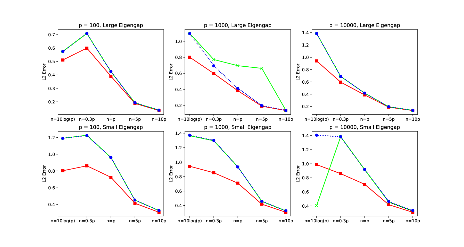
Refer to caption
Figure 9: The L2L_{2} Error for Different Algorithms on Simulated Matrix with Sparse principal eigenvector.
, Ordinary Power Iteration; , Truncated Power Iteration; , ElasticNet SPCA; , Algorithm 2 with Positive Cone.

Appendix B Preliminary Results

B.1 Constants

Below we define precisely the constants c−1c_{-1} and c1c_{1}. The intuition of defining such constants can be found in the proof of Lemma E.1. Let

cη\displaystyle c_{\eta} =k−‖E‖K+η​(k−‖E‖K)2−4​k​‖E‖K2​k, for ​η∈{−1,1}.\displaystyle=\frac{k-\|E\|_{K}+\eta\sqrt{(k-\|E\|_{K})^{2}-4k\|E\|_{K}}}{2k},\mbox{ for }\eta\in\{-1,1\}.

We have the following simple bounds for c−1c_{-1} and c1c_{1}.

Lemma B.1 (Bounds for c±1c_{\pm 1}).

Assuming that ν≥(3+2​2)​‖E‖K\nu\geq(3+2\sqrt{2})\|E\|_{K} we have the following relationships

‖E‖Kλ≤c−1≤(3+2​2)​‖E‖K(1+2)​ν​ and ​25<11+2≤c1.\displaystyle\frac{\|E\|_{K}}{\lambda}\leq c_{-1}\leq\frac{(3+2\sqrt{2})\|E\|_{K}}{(1+\sqrt{2})\nu}\,\,\,\,\mbox{ and }\hskip 9.24994pt\frac{2}{5}<\frac{1}{1+\sqrt{2}}\leq c_{1}.
Proof of Lemma B.1.

Note that c−1,c1c_{-1},c_{1} are well defined when ν≥(3+2​2)​‖E‖K\nu\geq(3+2\sqrt{2})\|E\|_{K}. Furthermore the following holds:

‖E‖Kλ≤‖E‖Kν−‖E‖K\displaystyle\frac{\|E\|_{K}}{\lambda}\leq\frac{\|E\|_{K}}{\nu-\|E\|_{K}} ≤2​‖E‖Kν−‖E‖K+(ν−‖E‖K)2−4​‖E‖K​k=c−1,\displaystyle\leq\frac{2\|E\|_{K}}{\nu-\|E\|_{K}+\sqrt{(\nu-\|E\|_{K})^{2}-4\|E\|_{K}k}}=c_{-1},
≤2​‖E‖Kν−‖E‖K≤(3+2​2)​‖E‖K(1+2)​ν,\displaystyle\leq\frac{2\|E\|_{K}}{\nu-\|E\|_{K}}\leq\frac{(3+2\sqrt{2})\|E\|_{K}}{(1+\sqrt{2})\nu},

In addition

c1≥k−‖E‖K2​ν>1+23+2​2=11+2.\displaystyle c_{1}\geq\frac{k-\|E\|_{K}}{2\nu}>\frac{1+\sqrt{2}}{3+2\sqrt{2}}=\frac{1}{1+\sqrt{2}}.

∎

Lemma B.2.

Under the assumption of Lemma B.1, if v0⊺​x¯>c−1v_{0}^{\intercal}\bar{x}>c_{-1} it follows that v0⊺​A​v0>0v_{0}^{\intercal}Av_{0}>0.

Proof of Lemma B.2.

Consider x¯⊺​A​v0≥λ​v0⊺​x¯−‖E‖K>λ​c−1−‖E‖K>0\bar{x}^{\intercal}Av_{0}\geq\lambda v_{0}^{\intercal}\bar{x}-\|E\|_{K}>\lambda c_{-1}-\|E\|_{K}>0 by Lemma B.1. Hence by Cauchy-Schwartz v0⊺​A​v0>0v_{0}^{\intercal}Av_{0}>0. ∎

B.2 Useful Tools

The following theorem states that any vector z∈ℝpz\in\mathbb{R}^{p} can be decomposed as the sum of its projection onto KK, and its projection onto KK’s polar cone K∘={u:⟨u,v⟩≤0,∀v∈K}K^{\circ}=\{u:\langle u,v\rangle\leq 0,\,\forall v\in K\}. It is a fundamental result in convex analysis.

Theorem B.1 ( (Moreau, 1962) (Moreau’s Decomposition)).

Let K⊂ℝpK\subset\mathbb{R}^{p} be a convex cone and KoK^{o} be its polar cone. For x,y,z∈ℝpx,y,z\in\mathbb{R}^{p}, the following properties are equivalent:

  1. 1.

    z=x+yz=x+y, x∈Kx\in K, y∈K∘y\in K^{\circ}, and ⟨x,y⟩=0\langle x,y\rangle=0.

  2. 2.

    x=ΠK​zx=\Pi_{K}z, y=ΠK∘​zy=\Pi_{K^{\circ}}z.

The following Lemma provides some equations and inequalities which will be referred a lot in consequent sections.

Lemma B.3.

Suppose that the vectors vtv_{t} are recursively defined as vt=ΠK​A​vt−1‖ΠK​A​vt−1‖v_{t}=\frac{\Pi_{K}Av_{t-1}}{\|\Pi_{K}Av_{t-1}\|}.

  1. 1.

    ‖ΠK​A​vt−1‖=vt⊺​A​vt−1\|\Pi_{K}Av_{t-1}\|=v_{t}^{\intercal}Av_{t-1}.

  2. 2.

    ∀x∈ℝp\forall x\in\mathbb{R}^{p}, x⊺​A¯​x≤(x¯⊺​x)2​λ+[1−(x¯⊺​x)2]​μx^{\intercal}\bar{A}x\leq(\bar{x}^{\intercal}x)^{2}\lambda+[1-(\bar{x}^{\intercal}x)^{2}]\mu.

  3. 3.

    ∀v∈K\forall v\in K we have |v⊺​E​v−x¯⊺​E​x¯|≤4​‖v−x¯‖​‖E‖𝒯K​(x¯)|v^{\intercal}Ev-\bar{x}^{\intercal}E\bar{x}|\leq 4\|v-\bar{x}\|\|E\|_{\mathcal{T}_{K}(\bar{x})} and |v⊺​E​v−x¯⊺​E​x¯|≤4​‖v+x¯‖​‖E‖K|v^{\intercal}Ev-\bar{x}^{\intercal}E\bar{x}|\leq 4\|v+\bar{x}\|\|E\|_{K}.

  4. 4.

    vt⊺​A​vt−1≤vt⊺​A​vtv_{t}^{\intercal}Av_{t-1}\leq v_{t}^{\intercal}Av_{t}.

Proof of Lemma B.3.
  1. 1.
    vt⊺​A​vt−1\displaystyle v_{t}^{\intercal}Av_{t-1} =⟨ΠK​A​vt−1,A​vt−1⟩‖ΠK​A​vt−1‖=⟨ΠK​A​vt−1,ΠK​A​vt−1⟩+⟨ΠK​A​vt−1,ΠK∘​A​vt−1⟩‖ΠK​A​vt−1‖\displaystyle=\frac{\langle\Pi_{K}Av_{t-1},Av_{t-1}\rangle}{\|\Pi_{K}Av_{t-1}\|}=\frac{\langle\Pi_{K}Av_{t-1},\Pi_{K}Av_{t-1}\rangle+\langle\Pi_{K}Av_{t-1},\Pi_{K^{\circ}}Av_{t-1}\rangle}{\|\Pi_{K}Av_{t-1}\|}
    =∥ΠKAvt−1∥by Moreau’s Decomposition\displaystyle=\|\Pi_{K}Av_{t-1}\|\hskip 18.49988pt\hskip 18.49988pt\text{by Moreau's Decomposition}
  2. 2.

    One can write xx as x=(x¯⊺​x)​x¯+1−(x¯⊺​x)2​x¯⟂x=(\bar{x}^{\intercal}x)\bar{x}+\sqrt{1-(\bar{x}^{\intercal}x)^{2}}\bar{x}^{\perp}. Then

    x⊺​A¯​x=(x¯⊺​x)2​λ+[1−(x¯⊺​x)2]​x¯⟂⁣⊺​A¯​x¯⟂≤(x¯⊺​x)2​λ+[1−(x¯⊺​x)2]​μ\displaystyle x^{\intercal}\bar{A}x=(\bar{x}^{\intercal}x)^{2}\lambda+[1-(\bar{x}^{\intercal}x)^{2}]\bar{x}^{\perp\intercal}\bar{A}\bar{x}^{\perp}\leq(\bar{x}^{\intercal}x)^{2}\lambda+[1-(\bar{x}^{\intercal}x)^{2}]\mu
  3. 3.

    On one hand

    |v⊺​E​v−x¯⊺​E​x¯|\displaystyle|v^{\intercal}Ev-\bar{x}^{\intercal}E\bar{x}| =|(v−x¯)⊺​E​(v−x¯)+2​x¯⊺​E​(v−x¯)|\displaystyle=|(v-\bar{x})^{\intercal}E(v-\bar{x})+2\bar{x}^{\intercal}E(v-\bar{x})|
    ≤‖v−x¯‖2​‖E‖𝒯K​(x¯)+2​‖v−x¯‖​‖E‖𝒯K​(x¯)\displaystyle\leq\|v-\bar{x}\|^{2}\|E\|_{\mathcal{T}_{K}(\bar{x})}+2\|v-\bar{x}\|\|E\|_{\mathcal{T}_{K}(\bar{x})}
    ≤4​‖v−x¯‖​‖E‖𝒯K​(x¯).\displaystyle\leq 4\|v-\bar{x}\|\|E\|_{\mathcal{T}_{K}(\bar{x})}.

    On the other hand,

    |v⊺​E​v−x¯⊺​E​x¯|≤|2​x¯⊺​E​(v+x¯)|+|(v+x¯)⊺​E​(v+x¯)|.\displaystyle|v^{\intercal}Ev-\bar{x}^{\intercal}E\bar{x}|\leq|2\bar{x}^{\intercal}E(v+\bar{x})|+|(v+\bar{x})^{\intercal}E(v+\bar{x})|.

    Since v+x¯∈Kv+\bar{x}\in K it follows that v+x¯‖v+x¯‖∈K\frac{v+\bar{x}}{\|v+\bar{x}\|}\in K and therefore

    |v⊺​E​v−x¯⊺​E​x¯|≤2​‖v+x¯‖​‖E‖K+‖v+x¯‖2​‖E‖K≤4​‖v+x¯‖​‖E‖K,\displaystyle|v^{\intercal}Ev-\bar{x}^{\intercal}E\bar{x}|\leq 2\|v+\bar{x}\|\|E\|_{K}+\|v+\bar{x}\|^{2}\|E\|_{K}\leq 4\|v+\bar{x}\|\|E\|_{K},
  4. 4.

    By Cauchy-Schwartz inequality we have

    vt⊺​A​vt−1≤(vt⊺​A​vt)​(vt−1⊺​A​vt−1)≤vt⊺​A​vt,\displaystyle v_{t}^{\intercal}Av_{t-1}\leq\sqrt{(v_{t}^{\intercal}Av_{t})(v_{t-1}^{\intercal}Av_{t-1})}\leq v_{t}^{\intercal}Av_{t},

    where vt⊺​A​vt≥vt−1⊺​A​vt−1v_{t}^{\intercal}Av_{t}\geq v_{t-1}^{\intercal}Av_{t-1} comes from the first part of the proof of Proposition 1.

∎

Appendix C Proof of Lemma 2.1

There are two definitions we need to introduce shortly. The first is the Orlicz norm ∥⋅∥ψα\|\cdot\|_{\psi_{\alpha}} of a random variable for 1≤α≤21\leq\alpha\leq 2

‖X‖ψα=inf{C>0:𝔼​exp⁡(|X/C|α)≤2}\displaystyle\|X\|_{\psi_{\alpha}}=\inf\{C>0:\,\mathbb{E}\exp(|X/C|^{\alpha})\leq 2\}

For a function ff defined on the probability space, Having a finite Orlicz norm is equivalent with displaying a tail behavior dominated by an exponential tail bound. If ‖X‖ψα<∞\|X\|_{\psi_{\alpha}}<\infty, one can show that ℙ⁡(|X|>t)≤2​exp(−ctα/∥X∥ψαα)\mathbb{P}(|X|>t)\leq 2\exp(-ct^{\alpha}/\|X\|_{\psi_\alpha}^{\alpha}) for c>0,t≥1c>0,t\geq 1. On the other hand, given ℙ⁡(|X|>t)≤2​exp(−tα/Cα)\mathbb{P}(|X|>t)\leq 2\exp(-t^{\alpha}/C^{\alpha}), one can show that ‖X‖ψα≤c1​C\|X\|_{\psi_{\alpha}}\leq c_{1}C for c1>0,C>0c_{1}>0,C>0. We say that XX is a sub-Exponential random variable if ‖X‖ψ1<∞\|X\|_{\psi_{1}}<\infty; a sub-Gaussian random variable if ‖X‖ψ2<∞\|X\|_{\psi_{2}}<\infty.

The second definition is the Talagrand’s γ2\gamma_{2} functional γ2​(T,d)\gamma_{2}(T,d), which measures the complexity of set TT with respect to metric dd. The quantity γ2​(T,d)\gamma_{2}(T,d) provides a link to the Gaussian Complexity of TT. The complete definition of γ2​(T,d)\gamma_{2}(T,d) can be found in Mendelson, 2010. Here we only need to know two properties of it

Lemma C.1.
  1. 1.

    For some constant k,Ck,C, if f:(T,d)→(U,d′)f:(T,d)\rightarrow(U,d^{\prime}) is onto and satisfies d′​(f⁡(x),f⁡(y))≤C​d​(x,y),∀x,y∈Td^{\prime}(f(x),f(y))\leq Cd(x,y),\,\,\forall x,y\in T, then γα​(U,d′)≤k​C​γα​(T,d)\gamma_{\alpha}(U,d^{\prime})\leq kC\gamma_{\alpha}(T,d) (Talagrand, 2006, Theorem 1.3.6).

  2. 2.

    Consider a Gaussian process {Xt}t∈T\{X_{t}\}_{t\in T} on TT, and the canonical distance d⁡(s,t)=𝔼​(Xt−Xs)2d(s,t)=\sqrt{\mathbb{E}(X_{t}-X_{s})^{2}}. For some universal constant cc we have γ2​(T,d)≤c​𝔼​supt∈TXt\gamma_{2}(T,d)\leq c\,\mathbb{E}\sup_{t\in T}X_{t} (Talagrand, 2006, Theorem 2.1.1).

Let start the proof of Lemma 2.1. The proof is based on Lemma C.2, which is an upper bound of the empirical process 𝔼​supf∈ℱ|1n​∑i=1nf2​(Zi)−𝔼​f2​(Zi)|\mathbb{E}\sup_{f\in\mathcal{F}}\big|\frac{1}{n}\sum_{i=1}^{n}f^{2}(Z_{i})-\mathbb{E}f^{2}(Z_{i})\big|. See Vu and Lei, 2012 and Mendelson, 2010.

Lemma C.2.

Let Zi,i=1,…,nZ_{i},i=1,...,n be i.i.d. random variables. There exists an absolute constant cc for which the following holds. If ℱ\mathcal{F} is a symmetric class of mean-zero functions then

𝔼​supf∈ℱ|1n​∑i=1nf2​(Zi)−𝔼​f2​(Zi)|≤c⁡[dψ1​γ2​(ℱ,ψ2)n∨γ22​(ℱ,ψ2)n]\displaystyle\mathbb{E}\sup_{f\in\mathcal{F}}\Big|\frac{1}{n}\sum_{i=1}^{n}f^{2}(Z_{i})-\mathbb{E}f^{2}(Z_{i})\Big|\leq c\big[d_{\psi_{1}}\frac{\gamma_{2}(\mathcal{F},\psi_{2})}{\sqrt{n}}\vee\frac{\gamma_{2}^{2}(\mathcal{F},\psi_{2})}{n}\big]

where dψ1=supf∈ℱ‖f‖ψ1d_{\psi_{1}}=\sup_{f\in\mathcal{F}}\|f\|_{\psi_{1}}.

1). Decompose ‖E‖K\|E\|_{K}
To apply Lemma C.2, we start with decomposing ‖E‖K\|E\|_{K}. Under the spiked covariance model, we have Xi∼𝒩⁡(0,I+ν​x¯​x¯⊺)X_{i}\sim\mathcal{N}(0,I+\nu\bar{x}\bar{x}^{\intercal}). Let 𝕏=[X1⊺;X2⊺;…;Xn⊺]\mathbb{X}=[X_{1}^{\intercal};X_{2}^{\intercal};...;X_{n}^{\intercal}]. With the fact I+ν​x¯​x¯⊺=I+(1+ν−1)​x¯​x¯⊺\sqrt{I+\nu\bar{x}\bar{x}^{\intercal}}=I+(\sqrt{1+\nu}-1)\bar{x}\bar{x}^{\intercal}, we can rewrite the noise matrix EE as

E\displaystyle E =A−A¯\displaystyle=A-\bar{A}
=𝕏⊺​𝕏n−(I+ν​x¯​x¯⊺)\displaystyle=\frac{\mathbb{X}^{\intercal}\mathbb{X}}{n}-(I+\nu\bar{x}\bar{x}^{\intercal})
=(I+(ν+1−1)​x¯​x¯⊺)​(X~⊺​X~n−I)​(I+(ν+1−1)​x¯​x¯⊺)\displaystyle=\big(I+(\sqrt{\nu+1}-1)\bar{x}\bar{x}^{\intercal}\big)\big(\frac{\tilde{X}^{\intercal}\tilde{X}}{n}-I\big)\big(I+(\sqrt{\nu+1}-1)\bar{x}\bar{x}^{\intercal}\big)

where X~\tilde{X} is a standard Gaussian matrix. Let ν0=ν+1−1\nu_{0}=\sqrt{\nu+1}-1, then

‖E‖K\displaystyle\|E\|_{K} =sup‖x‖=‖y‖=1,x,y∈K|x⊺​(I+ν0​x¯​x¯⊺)​(X~⊺​X~n−I)​(I+ν0​x¯​x¯⊺)​y|\displaystyle=\sup\limits_{\|x\|=\|y\|=1,\,\,x,y\in K}\Big|x^{\intercal}(I+\nu_{0}\bar{x}\bar{x}^{\intercal})(\frac{\tilde{X}^{\intercal}\tilde{X}}{n}-I)(I+\nu_{0}\bar{x}\bar{x}^{\intercal})y\Big|
=sup‖x‖=‖y‖=1,x,y∈K|[x+ν0​(x¯⊺​x)​x¯]⊺​(X~⊺​X~n−I)​[y+ν0​(x¯⊺​y)​x¯]|\displaystyle=\sup\limits_{\|x\|=\|y\|=1,\,\,x,y\in K}\Big|[x+\nu_{0}(\bar{x}^{\intercal}x)\bar{x}]^{\intercal}(\frac{\tilde{X}^{\intercal}\tilde{X}}{n}-I)[y+\nu_{0}(\bar{x}^{\intercal}y)\bar{x}]\Big|
≤sup‖x‖=‖y‖=1,x,y∈K|x⊺​(X~⊺​X~n−I)​y|+ν0​sup‖y‖=1,y∈K|x¯⊺​(X~⊺​X~n−I)​y|\displaystyle\leq\sup\limits_{\|x\|=\|y\|=1,\,\,x,y\in K}|x^{\intercal}(\frac{\tilde{X}^{\intercal}\tilde{X}}{n}-I)y|+\nu_{0}\sup\limits_{\|y\|=1,\,\,y\in K}|\bar{x}^{\intercal}(\frac{\tilde{X}^{\intercal}\tilde{X}}{n}-I)y|
+ν0sup‖x‖=1,x∈K|x¯⊺(X~⊺​X~n−I)x|+ν02|x¯⊺(X~⊺​X~n−I)x¯|\displaystyle+\nu_{0}\sup\limits_{\|x\|=1,\,\,x\in K}|\bar{x}^{\intercal}(\frac{\tilde{X}^{\intercal}\tilde{X}}{n}-I)x|+\nu_{0}^{2}|\bar{x}^{\intercal}(\frac{\tilde{X}^{\intercal}\tilde{X}}{n}-I)\bar{x}| (10)

With an algebraic trick one can show

sup‖x‖=‖y‖=1,x,y∈K|x⊺​(X~⊺​X~n−I)​y|\displaystyle\sup\limits_{\|x\|=\|y\|=1,\,\,x,y\in K}|x^{\intercal}(\frac{\tilde{X}^{\intercal}\tilde{X}}{n}-I)y|
=\displaystyle= sup‖x‖=‖y‖=1,x,y∈K12​|(x+y)⊺​(X~⊺​X~n−I)​(x+y)−x⊺​(X~⊺​X~n−I)​x−y⊺​(X~⊺​X~n−I)​y|\displaystyle\sup\limits_{\|x\|=\|y\|=1,\,\,x,y\in K}\frac{1}{2}|(x+y)^{\intercal}(\frac{\tilde{X}^{\intercal}\tilde{X}}{n}-I)(x+y)-x^{\intercal}(\frac{\tilde{X}^{\intercal}\tilde{X}}{n}-I)x-y^{\intercal}(\frac{\tilde{X}^{\intercal}\tilde{X}}{n}-I)y|
≤\displaystyle\leq sup‖x‖=‖y‖=1,x,y∈K12​|(x+y)⊺​(X~⊺​X~n−I)​(x+y)|+sup‖x‖=1,x∈K12​|x⊺​(X~⊺​X~n−I)​x|\displaystyle\sup\limits_{\|x\|=\|y\|=1,\,\,x,y\in K}\frac{1}{2}|(x+y)^{\intercal}(\frac{\tilde{X}^{\intercal}\tilde{X}}{n}-I)(x+y)|+\sup\limits_{\|x\|=1,\,\,x\in K}\frac{1}{2}|x^{\intercal}(\frac{\tilde{X}^{\intercal}\tilde{X}}{n}-I)x|
+sup‖y‖=1,y∈K12|y⊺(X~⊺​X~n−I)y|\displaystyle+\sup\limits_{\|y\|=1,\,\,y\in K}\frac{1}{2}|y^{\intercal}(\frac{\tilde{X}^{\intercal}\tilde{X}}{n}-I)y|

Let z=x+yz=x+y. Since KK is a convex cone, zz is also in KK. We have

sup‖x‖=‖y‖=1,x,y∈K12​|(x+y)⊺​(X~⊺​X~n−I)​(x+y)|\displaystyle\sup\limits_{\|x\|=\|y\|=1,\,\,x,y\in K}\frac{1}{2}|(x+y)^{\intercal}(\frac{\tilde{X}^{\intercal}\tilde{X}}{n}-I)(x+y)|
≤\displaystyle\leq sup‖z‖=2,z∈K12​|z⊺​(X~⊺​X~n−I)​z|=sup‖z‖=1,z∈K2​|z⊺​(X~⊺​X~n−I)​z|\displaystyle\sup\limits_{\|z\|=2,\,\,z\in K}\frac{1}{2}|z^{\intercal}(\frac{\tilde{X}^{\intercal}\tilde{X}}{n}-I)z|=\sup\limits_{\|z\|=1,\,\,z\in K}2|z^{\intercal}(\frac{\tilde{X}^{\intercal}\tilde{X}}{n}-I)z|

so that

sup‖x‖=‖y‖=1,x,y∈K|x⊺​(X~⊺​X~n−I)​y|≤3​sup‖x‖=1,x∈K|x⊺​(X~⊺​X~n−I)​x|\displaystyle\sup\limits_{\|x\|=\|y\|=1,\,\,x,y\in K}|x^{\intercal}(\frac{\tilde{X}^{\intercal}\tilde{X}}{n}-I)y|\leq 3\sup\limits_{\|x\|=1,\,\,x\in K}|x^{\intercal}(\frac{\tilde{X}^{\intercal}\tilde{X}}{n}-I)x|

The same trick can be applied to the other two terms sup‖y‖=1,y∈K|x¯⊺​(X~⊺​X~n−I)​y|\sup\limits_{\|y\|=1,\,\,y\in K}|\bar{x}^{\intercal}(\frac{\tilde{X}^{\intercal}\tilde{X}}{n}-I)y| and sup‖x‖=1,x∈K|x¯⊺​(X~⊺​X~n−I)​x|\sup\limits_{\|x\|=1,\,\,x\in K}|\bar{x}^{\intercal}(\frac{\tilde{X}^{\intercal}\tilde{X}}{n}-I)x| in (10):

sup‖x‖=1,x∈K|x¯⊺​(X~⊺​X~n−I)​x|\displaystyle\sup\limits_{\|x\|=1,\,\,x\in K}|\bar{x}^{\intercal}(\frac{\tilde{X}^{\intercal}\tilde{X}}{n}-I)x| ≤52​sup‖x‖=1,x∈K|x⊺​(X~⊺​X~n−I)​x|+12​|x¯⊺​(X~⊺​X~n−I)​x¯|\displaystyle\leq\frac{5}{2}\sup\limits_{\|x\|=1,\,\,x\in K}|x^{\intercal}(\frac{\tilde{X}^{\intercal}\tilde{X}}{n}-I)x|+\frac{1}{2}|\bar{x}^{\intercal}(\frac{\tilde{X}^{\intercal}\tilde{X}}{n}-I)\bar{x}|

so we can get

‖E‖K\displaystyle\|E\|_{K} ≤(5​ν0+3)​sup‖x‖=1,x∈K|x⊺​(X~⊺​X~n−I)​x|+(ν02+ν0)​|x¯⊺​(X~⊺​X~n−I)​x¯|\displaystyle\leq(5\nu_{0}+3)\sup\limits_{\|x\|=1,\,\,x\in K}|x^{\intercal}(\frac{\tilde{X}^{\intercal}\tilde{X}}{n}-I)x|+(\nu_{0}^{2}+\nu_{0})|\bar{x}^{\intercal}(\frac{\tilde{X}^{\intercal}\tilde{X}}{n}-I)\bar{x}|

2). Bound 𝔼​|x¯⊺​(X~⊺​X~n−I)​x¯|\mathbb{E}|\bar{x}^{\intercal}(\frac{\tilde{X}^{\intercal}\tilde{X}}{n}-I)\bar{x}|.
Notice that x¯⊺​(X~⊺​X~n−I)​x¯=1n​∑i=1n[(X~​x¯)i2−1]\bar{x}^{\intercal}(\frac{\tilde{X}^{\intercal}\tilde{X}}{n}-I)\bar{x}=\frac{1}{n}\sum\limits_{i=1}^{n}[(\tilde{X}\bar{x})^{2}_{i}-1], and (X~​x¯)i2∼χ12(\tilde{X}\bar{x})^{2}_{i}\sim\chi_{1}^{2}. Let Z=1n​∑i=1n[(X​v)i2−1]Z=\frac{1}{n}\sum\limits_{i=1}^{n}[(Xv)^{2}_{i}-1]. The following concentration inequalities hold for ZZ (Laurent and Massart, 2000, Lemma 1),

ℙ⁡(ZCLOSE\displaystyle\mathbb{P}\big(Z OPEN≥2​xn+2​xn)≤e−x\displaystyle\geq 2\sqrt{\frac{x}{n}}+2\frac{x}{n}\big)\leq e^{-x}
ℙ⁡(ZCLOSE\displaystyle\mathbb{P}\big(Z OPEN≤−2​xn)≤e−x\displaystyle\leq-2\sqrt{\frac{x}{n}}\big)\leq e^{-x}

so that

ℙ⁡(n​Z≥t)\displaystyle\mathbb{P}\big(\sqrt{n}Z\geq t\big) ≤e−t216if ​t<4​n\displaystyle\leq e^{-\frac{t^{2}}{16}}\hskip 18.49988pt\text{if }t<4\sqrt{n}
ℙ⁡(n​Z≥t)\displaystyle\mathbb{P}\big(\sqrt{n}Z\geq t\big) ≤e−n​t4if ​t≥4​n\displaystyle\leq e^{-\frac{\sqrt{n}t}{4}}\hskip 18.49988pt\text{if }t\geq 4\sqrt{n}
ℙ⁡(n​Z≤−t)\displaystyle\mathbb{P}\big(\sqrt{n}Z\leq-t\big) ≤e−t24\displaystyle\leq e^{-\frac{t^{2}}{4}}

The expectation can be bounded as

𝔼​|n​Z|\displaystyle\mathbb{E}|\sqrt{n}Z| =∫0∞ℙ⁡(n​|Z|>t)​𝑑t\displaystyle=\int_{0}^{\infty}\mathbb{P}(\sqrt{n}|Z|>t)dt
=∫t<4​ne−t216​𝑑t+∫t>4​ne−n​t4​𝑑t\displaystyle=\int_{t<4\sqrt{n}}e^{-\frac{t^{2}}{16}}dt+\int_{t>4\sqrt{n}}e^{-\frac{\sqrt{n}t}{4}}dt
≤∫−∞+∞e−t216​𝑑t−4n​e−n​t4|4​n+∞\displaystyle\leq\int_{-\infty}^{+\infty}e^{-\frac{t^{2}}{16}}dt-\frac{4}{\sqrt{n}}e^{-\frac{\sqrt{n}t}{4}}\Big|_{4\sqrt{n}}^{+\infty}
=4​π+4n​e−n2\displaystyle=4\sqrt{\pi}+\frac{4}{\sqrt{n}}e^{-n^{2}}

thus

𝔼​|Z|≲1/n\displaystyle\mathbb{E}|Z|\lesssim 1/\sqrt{n}

3). Bound 𝔼​sup‖x‖=1,x∈K|x⊺​(X~⊺​X~n−I)​x|\mathbb{E}\sup\limits_{\|x\|=1,\,\,x\in K}|x^{\intercal}(\frac{\tilde{X}^{\intercal}\tilde{X}}{n}-I)x|.
Let Xi~\tilde{X_{i}} be the ii-th row of the matrix X~\tilde{X}. Since X~\tilde{X} is a standard Gaussian matrix, Xi~\tilde{X_{i}} is a pp-dimensional standard Gaussian vector. We have

𝔼​sup‖x‖=1,x∈K|x⊺​(X~⊺​X~n−I)​x|\displaystyle\mathbb{E}\sup\limits_{\|x\|=1,\,\,x\in K}|x^{\intercal}(\frac{\tilde{X}^{\intercal}\tilde{X}}{n}-I)x| =𝔼​sup‖x‖=1,x∈K|x⊺​(1n​∑i=1nXi~​Xi~⊺−I)​x|\displaystyle=\mathbb{E}\sup\limits_{\|x\|=1,\,\,x\in K}|x^{\intercal}(\frac{1}{n}\sum_{i=1}^{n}\tilde{X_{i}}\tilde{X_{i}}^{\intercal}-I)x|
=𝔼​sup‖x‖=1,x∈K|1n​∑i=1n⟨Xi~,x⟩2−𝔼​⟨Xi~,x⟩2|\displaystyle=\mathbb{E}\sup\limits_{\|x\|=1,\,\,x\in K}|\frac{1}{n}\sum_{i=1}^{n}\langle\tilde{X_{i}},x\rangle^{2}-\mathbb{E}\langle\tilde{X_{i}},x\rangle^{2}|

Define a class of linear functionals ℱ≔{⟨,v⟩,v∈K⋂𝕊p−1}\mathcal{F}\coloneqq\{\langle,v\rangle,\,\,v\in K\bigcap\mathbb{S}^{p-1}\}. The above quantity can be written as 𝔼​supf∈ℱ 2​|1n​∑i=1nf2​(Xi~)−𝔼​f2​(Xi~)|\mathbb{E}\sup_{f\in\mathcal{F}}\,2\Big|\frac{1}{n}\sum_{i=1}^{n}f^{2}(\tilde{X_{i}})-\mathbb{E}f^{2}(\tilde{X_{i}})\Big|, which fits in the setting of Lemma C.2.

Now we decode the abstract RHS of Lemma C.2 into an explicit expression related to the Gaussian Complexity w⁡(K​⋂𝕊p−1)w(K\bigcap\mathbb{S}^{p-1}). First we bound dψ1d_{\psi_{1}}. For a constant c1c_{1}

dψ1\displaystyle d_{\psi_{1}} =supv∈K​⋂𝕊p−1‖⟨Xi~,v⟩‖ψ1\displaystyle=\sup_{v\in K\bigcap\mathbb{S}^{p-1}}\|\langle\tilde{X_{i}},v\rangle\|_{\psi_{1}}
≤c1​supv∈K​⋂𝕊p−1‖⟨Xi~,v⟩‖ψ2\displaystyle\leq c_{1}\sup_{v\in K\bigcap\mathbb{S}^{p-1}}\|\langle\tilde{X_{i}},v\rangle\|_{\psi_{2}}

Since Xi~\tilde{X_{i}} is a standard normal random variable, we have

‖⟨Xi~,v⟩‖ψ2≤83​‖v‖2≤83\displaystyle\|\langle\tilde{X_{i}},v\rangle\|_{\psi_{2}}\leq\sqrt{\frac{8}{3}}\|v\|_{2}\leq\sqrt{\frac{8}{3}}

and so

dψ1\displaystyle d_{\psi_{1}} ≤c1​83\displaystyle\leq c_{1}\sqrt{\frac{8}{3}}

Then we bound γ2​(ℱ,ψ2)\gamma_{2}(\mathcal{F},\psi_{2}) by the Gaussian Complexity w⁡(K​⋂𝕊p−1)w(K\bigcap\mathbb{S}^{p-1}). Notice that the metric induced by the ψ2\psi_{2}-norm on ℱ\mathcal{F} is equivalent with the Euclidean distance on K​⋂𝕊p−1K\bigcap\mathbb{S}^{p-1}

‖(f−g)​(Xi~)‖ψ2=‖⟨Xi~,(vf−vg)⟩‖ψ2≤83​‖vf−vg‖2\displaystyle\|(f-g)(\tilde{X_{i}})\|_{\psi_{2}}=\|\langle\tilde{X_{i}},(v_{f}-v_{g})\rangle\|_{\psi_{2}}\leq\sqrt{\frac{8}{3}}\|v_{f}-v_{g}\|_{2}

where f,g∈ℱf,g\in\mathcal{F} and vf,vg∈K​⋂𝕊p−1v_{f},v_{g}\in K\bigcap\mathbb{S}^{p-1}. By the first result of Lemma C.1, for a constant c2c_{2}

γ2(ℱ,ψ2)≤c283γ2(K⋂𝕊p−1,∥⋅∥2)\displaystyle\gamma_{2}(\mathcal{F},\psi_{2})\leq c_{2}\,\sqrt{\frac{8}{3}}\,\gamma_{2}(K\bigcap\mathbb{S}^{p-1},\|\cdot\|_{2})

And by the second result of Lemma C.1, for some constant c3c_{3}

γ2​(ℱ,ψ2)≤c2​c3​83​𝔼​supv∈K​⋂𝕊p−1⟨Z,v⟩\displaystyle\gamma_{2}(\mathcal{F},\psi_{2})\leq c_{2}c_{3}\sqrt{\frac{8}{3}}\,\,\mathbb{E}\sup_{v\in K\bigcap\mathbb{S}^{p-1}}\langle Z,v\rangle

where ZZ is a pp-dimensional standard Gaussian random vector. And according to the definition of Gaussian Complexity w⁡(K​⋂𝕊p−1)=supv∈K​⋂𝕊p−1⟨Z,v⟩w(K\bigcap\mathbb{S}^{p-1})=\sup_{v\in K\bigcap\mathbb{S}^{p-1}}\langle Z,v\rangle. Thus

𝔼​sup‖x‖=1,x∈K|x⊺​(X~⊺​X~n−I)​x|\displaystyle\mathbb{E}\sup\limits_{\|x\|=1,\,\,x\in K}|x^{\intercal}(\frac{\tilde{X}^{\intercal}\tilde{X}}{n}-I)x| =𝔼​supf∈ℱ|1n​∑i=1nf2​(Zi)−𝔼​f2​(Zi)|\displaystyle=\mathbb{E}\sup_{f\in\mathcal{F}}\,\Big|\frac{1}{n}\sum_{i=1}^{n}f^{2}(Z_{i})-\mathbb{E}f^{2}(Z_{i})\Big|
≤c⁡[dψ1​γ2​(ℱ,ψ2)n∨γ22​(ℱ,ψ2)n]\displaystyle\leq c\big[d_{\psi_{1}}\frac{\gamma_{2}(\mathcal{F},\psi_{2})}{\sqrt{n}}\vee\frac{\gamma_{2}^{2}(\mathcal{F},\psi_{2})}{n}\big]
≤c​c2​c3​83​[c1​w​(K​⋂𝕊p−1)n∨c2​c3​w2​(K​⋂𝕊p−1)n]\displaystyle\leq cc_{2}c_{3}\frac{8}{3}\bigg[\frac{c_{1}w(K\bigcap\mathbb{S}^{p-1})}{\sqrt{n}}\vee\frac{c_{2}c_{3}w^{2}(K\bigcap\mathbb{S}^{p-1})}{n}\bigg]
≲w⁡(K​⋂𝕊p−1)n∨w2​(K​⋂𝕊p−1)n\displaystyle\lesssim\frac{w(K\bigcap\mathbb{S}^{p-1})}{\sqrt{n}}\vee\frac{w^{2}(K\bigcap\mathbb{S}^{p-1})}{n}

4). Bound 𝔼​‖E‖K\mathbb{E}\|E\|_{K}.
Finally we can get

𝔼​‖E‖K\displaystyle\mathbb{E}\|E\|_{K} ≲(5​ν0+3)​[w⁡(K​⋂𝕊p−1)n∨w2​(K​⋂𝕊p−1)n]+(ν02+ν0)​1n\displaystyle\lesssim(5\nu_{0}+3)\bigg[\frac{w(K\bigcap\mathbb{S}^{p-1})}{\sqrt{n}}\vee\frac{w^{2}(K\bigcap\mathbb{S}^{p-1})}{n}\bigg]+(\nu_{0}^{2}+\nu_{0})\frac{1}{\sqrt{n}}

Plug in ν0=ν+1−1\nu_{0}=\sqrt{\nu+1}-1 to get

𝔼​‖E‖K\displaystyle\mathbb{E}\|E\|_{K} ≲(5​ν+1−2)​[w⁡(K​⋂𝕊p−1)n∨w2​(K​⋂𝕊p−1)n]+ν+3−3​ν+1n\displaystyle\lesssim(5\sqrt{\nu+1}-2)\bigg[\frac{w(K\bigcap\mathbb{S}^{p-1})}{\sqrt{n}}\vee\frac{w^{2}(K\bigcap\mathbb{S}^{p-1})}{n}\bigg]+\frac{\nu+3-3\sqrt{\nu+1}}{\sqrt{n}}
≲ν+1​[w⁡(K​⋂𝕊p−1)n∨w2​(K​⋂𝕊p−1)n]+ν+3−3​ν+1n\displaystyle\lesssim\sqrt{\nu+1}\bigg[\frac{w(K\bigcap\mathbb{S}^{p-1})}{\sqrt{n}}\vee\frac{w^{2}(K\bigcap\mathbb{S}^{p-1})}{n}\bigg]+\frac{\nu+3-3\sqrt{\nu+1}}{\sqrt{n}}

Appendix D Proof of Theorem 3.1 and Corollary 3.1

D.1 Proof of Theorem 3.1

Suppose first that v⊺​x¯≥0v^{\intercal}\bar{x}\geq 0.

v⊺​E​v−x¯⊺​E​x¯\displaystyle v^{\intercal}Ev-\bar{x}^{\intercal}E\bar{x} =v⊺​A​v⊺−v⊺​A¯​v−(x¯​A​x¯−x¯​A¯​x¯)\displaystyle=v^{\intercal}Av^{\intercal}-v^{\intercal}\bar{A}v-(\bar{x}A\bar{x}-\bar{x}\bar{A}\bar{x})
≥x¯​A¯​x¯−v⊺​A¯​v\displaystyle\geq\bar{x}\bar{A}\bar{x}-v^{\intercal}\bar{A}v
≥λ−(v⊺x¯)2λ−[1−(v⊺x¯)2]μBy 2. in Lemma B.3\displaystyle\geq\lambda-(v^{\intercal}\bar{x})^{2}\lambda-[1-(v^{\intercal}\bar{x})^{2}]\mu\hskip 18.49988pt\hskip 18.49988pt\hskip 9.24994pt\text{By 2. in Lemma \ref{ineqs}}
≥ν⁡[1−(v⊺​x¯)2]\displaystyle\geq\nu[1-(v^{\intercal}\bar{x})^{2}]
≥12​ν​‖v−x¯‖2\displaystyle\geq\frac{1}{2}\nu\|v-\bar{x}\|^{2}

For the first term, by the definition of ‖E‖K\|E\|_{K}, we can directly get v⊺​E​v−x¯⊺​E​x¯≤2​‖E‖Kv^{\intercal}Ev-\bar{x}^{\intercal}E\bar{x}\leq 2\|E\|_{K}. For the second term, notice that

v⊺​E​v−x¯⊺​E​x¯≤4​‖v−x¯‖​‖E‖𝒯K​(x¯)By 3. in Lemma B.3\displaystyle v^{\intercal}Ev-\bar{x}^{\intercal}E\bar{x}\leq 4\|v-\bar{x}\|\|E\|_{\mathcal{T}_{K}(\bar{x})}\hskip 18.49988pt\hskip 18.49988pt\hskip 9.24994pt\text{By 3. in Lemma \ref{ineqs}}

so

12​ν​‖v−x¯‖2≤4​‖v−x¯‖​‖E‖𝒯K​(x¯)⇒‖v−x¯‖≤8​‖E‖𝒯K​(x¯)ν\displaystyle\frac{1}{2}\nu\|v-\bar{x}\|^{2}\leq 4\|v-\bar{x}\|\|E\|_{\mathcal{T}_{K}(\bar{x})}\hskip 18.49988pt\Rightarrow\hskip 18.49988pt\|v-\bar{x}\|\leq\frac{8\|E\|_{\mathcal{T}_{K}(\bar{x})}}{\nu}

Next suppose that v⊺​x¯≤0v^{\intercal}\bar{x}\leq 0. Repeating the same proof as above we observe that

v⊺​E​v−x¯⊺​E​x¯≥12​ν​‖v+x¯‖2.\displaystyle v^{\intercal}Ev-\bar{x}^{\intercal}E\bar{x}\geq\frac{1}{2}\nu\|v+\bar{x}\|^{2}.

This and the bound v⊺​E​v−x¯⊺​E​x¯≤2​‖E‖Kv^{\intercal}Ev-\bar{x}^{\intercal}E\bar{x}\leq 2\|E\|_{K} directly give the proof of one of the inequalities. Next by 3. in Lemma B.3 we have

v⊺​E​v−x¯⊺​E​x¯≤4​‖v+x¯‖​‖E‖K\displaystyle v^{\intercal}Ev-\bar{x}^{\intercal}E\bar{x}\leq 4\|v+\bar{x}\|\|E\|_{K}

which implies the second bound.

D.2 Proof of Corollary 3.1

It is sufficient to show ‖E‖𝒯K​(x¯)∨‖E‖K≤‖E‖o​p\|E\|_{\mathcal{T}_{K}(\bar{x})}\vee\|E\|_{K}\leq\|E\|_{op}. This is obvious by the definitions of ‖E‖𝒯K​(x¯)\|E\|_{\mathcal{T}_{K}(\bar{x})} and ‖E‖K\|E\|_{K}.

Appendix E Proof of Theorem 4.1 and Theorem 4.2

A key to analyze the L2L_{2} error of the cone projected power iteration estimator is: If x¯⊺​v0\bar{x}^{\intercal}v_{0} is larger than a certain constant, x¯⊺​vt\bar{x}^{\intercal}v_{t} is always larger than that constant throughout the iterations. This is rigorously presented in the following lemma E.1. It is a foundation for the proof of Theorem 4.1.

Lemma E.1.

Suppose x¯⊺​v0≥c0\bar{x}^{\intercal}v_{0}\geq c_{0} for some c0>c−1c_{0}>c_{-1}, and the first eigengap of A¯\bar{A} is greater than (3+2​2)​‖E‖K(3+2\sqrt{2})\|E\|_{K}, then x¯⊺​vt≥c0∧c1,∀t∈ℕ\bar{x}^{\intercal}v_{t}\geq c_{0}\wedge c_{1},\,\,\forall t\in\mathbb{N}.

Proof of Lemma E.1.

We prove this result by induction.

Given x¯⊺​vt−1≥c0\bar{x}^{\intercal}v_{t-1}\geq c_{0}, if x¯⊺​vt≥x¯⊺​vt−1\bar{x}^{\intercal}v_{t}\geq\bar{x}^{\intercal}v_{t-1}, the inequality preserves trivially.

Next suppose that x¯⊺​vt≤x¯⊺​vt−1\bar{x}^{\intercal}v_{t}\leq\bar{x}^{\intercal}v_{t-1}. We first show that x¯⊺​vt\bar{x}^{\intercal}v_{t} is non-negative. We have the identity x¯⊺​vt=x¯⊺​ΠK​A​vt−1‖ΠK​A​vt−1‖\bar{x}^{\intercal}v_{t}=\frac{\bar{x}^{\intercal}\Pi_{K}Av_{t-1}}{\|\Pi_{K}Av_{t-1}\|}, so it suffices to show that x¯⊺​ΠK​A​vt−1≥x¯⊺​A​vt−1≥λ​x¯⊺​vt−1−‖E‖K≥0\bar{x}^{\intercal}\Pi_{K}Av_{t-1}\geq\bar{x}^{\intercal}Av_{t-1}\geq\lambda\bar{x}^{\intercal}v_{t-1}-\|E\|_{K}\geq 0, which holds since x¯⊺​vt−1≥c0∧c1>c−1≥‖E‖Kλ\bar{x}^{\intercal}v_{t-1}\geq c_{0}\wedge c_{1}>c_{-1}\geq\frac{\|E\|_{K}}{\lambda} (the last inequality is shown in Lemma B.1).

Next observe the identities,

x¯⊺​vt\displaystyle\bar{x}^{\intercal}v_{t} =x¯⊺​ΠK​A​vt−1‖ΠK​A​vt−1‖≥x¯⊺​A​vt−1vt⊺​A​vt−1By Moreau’s decomposition and 1. in Lemma B.3\displaystyle=\frac{\bar{x}^{\intercal}\Pi_{K}Av_{t-1}}{\|\Pi_{K}Av_{t-1}\|}\,\geq\frac{\bar{x}^{\intercal}Av_{t-1}}{v_{t}^{\intercal}Av_{t-1}}\hskip 9.24994pt\hskip 9.24994pt\,\,\text{By Moreau's decomposition and 1. in Lemma \ref{ineqs}}
≥x¯⊺​A​vt−1vt⊺​A​vt By 4. in Lemma B.3\displaystyle\geq\frac{\bar{x}^{\intercal}Av_{t-1}}{v_{t}^{\intercal}Av_{t}}\hskip 9.24994pt\hskip 9.24994pt\hskip 9.24994pt\hskip 9.24994pt\hskip 9.24994pt\hskip 9.24994pt\hskip 9.24994pt\hskip 9.24994pt\hskip 9.24994pt\text{ By 4. in Lemma \ref{ineqs}}
≥x¯⊺​A¯​vt−1−‖E‖Kvt⊺​A¯​vt+‖E‖K\displaystyle\geq\frac{\bar{x}^{\intercal}\bar{A}v_{t-1}-\|E\|_{K}}{v_{t}^{\intercal}\bar{A}v_{t}+\|E\|_{K}}
≥λ​x¯⊺​vt−1−‖E‖K(x¯⊺​vt)2​λ+[1−(x¯⊺​vt)2]​μ+‖E‖KBy 2. in Lemma B.3\displaystyle\geq\frac{\lambda\bar{x}^{\intercal}v_{t-1}-\|E\|_{K}}{(\bar{x}^{\intercal}v_{t})^{2}\lambda+[1-(\bar{x}^{\intercal}v_{t})^{2}]\mu+\|E\|_{K}}\hskip 18.49988pt\hskip 18.49988pt\hskip 18.49988pt\hskip 18.49988pt\hskip 9.24994pt\text{By 2. in Lemma \ref{ineqs}}
≥λ​x¯⊺​vt−1−‖E‖Kν⁡(x¯⊺​vt−1)+μ+‖E‖KBy the condition 0≤x¯⊺​vt≤x¯⊺​vt−1\displaystyle\geq\frac{\lambda\bar{x}^{\intercal}v_{t-1}-\|E\|_{K}}{\nu(\bar{x}^{\intercal}v_{t-1})+\mu+\|E\|_{K}}\hskip 18.49988pt\hskip 18.49988pt\hskip 18.49988pt\hskip 18.49988pt\hskip 9.24994pt\hskip 18.49988pt\hskip 18.49988pt\hskip 9.24994pt\text{By the condition $0\leq\bar{x}^{\intercal}v_{t}\leq\bar{x}^{\intercal}v_{t-1}$}

Let α=x¯⊺​vt−1\alpha=\bar{x}^{\intercal}v_{t-1}, and f⁡(y)=λ​y−‖E‖Kν​y+μ+‖E‖Kf(y)=\frac{\lambda y-\|E\|_{K}}{\nu y+\mu+\|E\|_{K}}. Note that the roots of the quadratic equation f⁡(y)=yf(y)=y are c−1c_{-1} and c1c_{1}, so that for y∈(−∞,c−1]⋃[c1,∞)y\in(-\infty,c_{-1}]\bigcup[c_{1},\infty), we have y≥f⁡(y)y\geq f(y). By the fact that α=x¯⊺​vt−1≥f⁡(α)\alpha=\bar{x}^{\intercal}v_{t-1}\geq f(\alpha) and α≥c0∧c1>c−1\alpha\geq c_{0}\wedge c_{1}>c_{-1}, it follows that α≥c1\alpha\geq c_{1}. In addition since x¯⊺​vt≥f⁡(α)\bar{x}^{\intercal}v_{t}\geq f(\alpha), it is sufficient to show f⁡(α)≥c0∧c1f(\alpha)\geq c_{0}\wedge c_{1}. Notice that f⁡(y)f(y) is increasing, so f⁡(α)≥f⁡(c1)=c1≥c0∧c1f(\alpha)\geq f(c_{1})=c_{1}\geq c_{0}\wedge c_{1}. Thus the proof is complete. ∎

E.1 Proof of Theorem 4.1

For the first term, we can start to derive a lower bound and an upper bound of x¯⊺​A​vt−1\bar{x}^{\intercal}Av_{t-1} based on some inequalities from Lemma B.3,

x¯⊺​A​vt−1\displaystyle\bar{x}^{\intercal}Av_{t-1} =λ​x¯⊺​vt−1+x¯⊺​E​vt−1≥λ​x¯⊺​vt−1−‖E‖K\displaystyle=\lambda\bar{x}^{\intercal}v_{t-1}+\bar{x}^{\intercal}Ev_{t-1}\geq\lambda\bar{x}^{\intercal}v_{t-1}-\|E\|_{K}
x¯⊺​A​vt−1\displaystyle\bar{x}^{\intercal}Av_{t-1} =x¯⊺​ΠK​A​vt−1+x¯⊺​ΠK∘​A​vt−1≤x¯⊺​ΠK​A​vt−1=‖ΠK​A​vt−1‖​x¯⊺​vt=(vt⊺​A​vt−1)​x¯⊺​vt\displaystyle=\bar{x}^{\intercal}\Pi_{K}Av_{t-1}+\bar{x}^{\intercal}\Pi_{K^{\circ}}Av_{t-1}\leq\bar{x}^{\intercal}\Pi_{K}Av_{t-1}=\|\Pi_{K}Av_{t-1}\|\bar{x}^{\intercal}v_{t}=(v_{t}^{\intercal}Av_{t-1})\bar{x}^{\intercal}v_{t}

Combine the above two inequalities to get

λ​x¯⊺​vt−1−‖E‖K\displaystyle\lambda\bar{x}^{\intercal}v_{t-1}-\|E\|_{K} ≤(vt⊺​A​vt−1)​x¯⊺​vt=(vt⊺​A​vt−1)​x¯⊺​vt−1+(vt⊺​A​vt−1)​x¯⊺​(vt−vt−1)\displaystyle\leq(v_{t}^{\intercal}Av_{t-1})\bar{x}^{\intercal}v_{t}=(v_{t}^{\intercal}Av_{t-1})\bar{x}^{\intercal}v_{t-1}+(v_{t}^{\intercal}Av_{t-1})\bar{x}^{\intercal}(v_{t}-v_{t-1}) (11)

Since ‖vt−vt−1‖≤Δ\|v_{t}-v_{t-1}\|\leq\Delta, by Cauchy-Schwartz inequality and the definition of ‖E‖K\|E\|_{K},

(vt⊺​A​vt−1)​x¯⊺​(vt−vt−1)\displaystyle(v_{t}^{\intercal}Av_{t-1})\bar{x}^{\intercal}(v_{t}-v_{t-1}) ≤|vt⊺​A¯​vt−1+vt⊺​E​vt−1|​‖vt−vt−1‖\displaystyle\leq|v_{t}^{\intercal}\bar{A}v_{t-1}+v_{t}^{\intercal}Ev_{t-1}|\,\|v_{t}-v_{t-1}\|
≤(λ+‖E‖K)​Δ\displaystyle\leq(\lambda+\|E\|_{K})\Delta

Furthermore, with the use of results in Lemma B.3,

(vt⊺​A​vt−1)​x¯⊺​vt−1\displaystyle(v_{t}^{\intercal}Av_{t-1})\bar{x}^{\intercal}v_{t-1} =(vt⊺​A¯​vt−1+vt⊺​E​vt−1)​x¯⊺​vt−1\displaystyle=(v_{t}^{\intercal}\bar{A}v_{t-1}+v_{t}^{\intercal}Ev_{t-1})\bar{x}^{\intercal}v_{t-1}
≤(vt⊺​A¯​vt+(vt−1−vt)⊺​A¯​vt+‖E‖K)​x¯⊺​vt−1\displaystyle\leq\big(v_{t}^{\intercal}\bar{A}v_{t}+(v_{t-1}-v_{t})^{\intercal}\bar{A}v_{t}+\|E\|_{K}\big)\bar{x}^{\intercal}v_{t-1}
≤(vt⊺​A¯​vt)​x¯⊺​vt−1+(‖vt−1−vt‖​‖A¯​vt‖+‖E‖K)​x¯⊺​vt−1\displaystyle\leq(v_{t}^{\intercal}\bar{A}v_{t})\bar{x}^{\intercal}v_{t-1}+\big(\|v_{t-1}-v_{t}\|\,\|\bar{A}v_{t}\|+\|E\|_{K}\big)\bar{x}^{\intercal}v_{t-1}
≤(vt⊺​A¯​vt)​x¯⊺​vt−1+(Δ​λ+‖E‖K)​x¯⊺​vt−1\displaystyle\leq(v_{t}^{\intercal}\bar{A}v_{t})\bar{x}^{\intercal}v_{t-1}+\big(\Delta\lambda+\|E\|_{K}\big)\bar{x}^{\intercal}v_{t-1}
≤[λ​(x¯⊺​vt)2+μ⁡(1−(x¯⊺​vt)2)]​x¯⊺​vt−1+(Δ​λ+‖E‖K)​x¯⊺​vt−1\displaystyle\leq\big[\lambda(\bar{x}^{\intercal}v_{t})^{2}+\mu\big(1-(\bar{x}^{\intercal}v_{t})^{2}\big)\big]\bar{x}^{\intercal}v_{t-1}+\big(\Delta\lambda+\|E\|_{K}\big)\bar{x}^{\intercal}v_{t-1}

Thus (11) becomes

λ​x¯⊺​vt−1−‖E‖K\displaystyle\lambda\bar{x}^{\intercal}v_{t-1}-\|E\|_{K} ≤[λ​(x¯⊺​vt)2+μ⁡(1−(x¯⊺​vt)2)]​x¯⊺​vt−1+(Δ​λ+‖E‖K)​x¯⊺​vt−1+(λ+‖E‖K)​Δ\displaystyle\leq\big[\lambda(\bar{x}^{\intercal}v_{t})^{2}+\mu\big(1-(\bar{x}^{\intercal}v_{t})^{2}\big)\big]\bar{x}^{\intercal}v_{t-1}+\big(\Delta\lambda+\|E\|_{K}\big)\bar{x}^{\intercal}v_{t-1}+(\lambda+\|E\|_{K})\Delta
⇒ν⁡[1−(x¯⊺​vt)2]​x¯⊺​vt−1\displaystyle\Rightarrow\hskip 9.24994pt\nu[1-(\bar{x}^{\intercal}v_{t})^{2}]\bar{x}^{\intercal}v_{t-1} ≤(Δ​λ+‖E‖K)​x¯⊺​vt−1+(λ+‖E‖K)​Δ+‖E‖K\displaystyle\leq\big(\Delta\lambda+\|E\|_{K}\big)\bar{x}^{\intercal}v_{t-1}+(\lambda+\|E\|_{K})\Delta+\|E\|_{K}

According to Lemma E.1, x¯⊺​vt≥c0∧c1≥0\bar{x}^{\intercal}v_{t}\geq c_{0}\wedge c_{1}\geq 0, so 1−(x¯⊺​vt)2≥1−x¯⊺​vt=12​‖vt−x¯‖21-(\bar{x}^{\intercal}v_{t})^{2}\geq 1-\bar{x}^{\intercal}v_{t}=\frac{1}{2}\|v_{t}-\bar{x}\|^{2}, thus

ν2​‖vt−x¯‖2​x¯⊺​vt−1\displaystyle\frac{\nu}{2}\|v_{t}-\bar{x}\|^{2}\bar{x}^{\intercal}v_{t-1} ≤(Δ​λ+‖E‖K)​x¯⊺​vt−1+(λ+‖E‖K)​Δ+‖E‖K\displaystyle\leq\big(\Delta\lambda+\|E\|_{K}\big)\bar{x}^{\intercal}v_{t-1}+(\lambda+\|E\|_{K})\Delta+\|E\|_{K}

Since c0∧c1≤x¯⊺​vt−1≤1c_{0}\wedge c_{1}\leq\bar{x}^{\intercal}v_{t-1}\leq 1 and Δ≤‖E‖K2​λ∧1\Delta\leq\frac{\|E\|_{K}}{2\lambda}\wedge 1,

ν2​‖vt−x¯‖2​(c0∧c1)\displaystyle\frac{\nu}{2}\|v_{t}-\bar{x}\|^{2}(c_{0}\wedge c_{1}) ≤(Δ​λ+‖E‖K)+(λ+‖E‖K)​Δ+‖E‖K\displaystyle\leq\big(\Delta\lambda+\|E\|_{K}\big)+(\lambda+\|E\|_{K})\Delta+\|E\|_{K}
≤4​‖E‖K\displaystyle\leq 4\|E\|_{K}
⇒‖vt−x¯‖\displaystyle\Rightarrow\hskip 9.24994pt\|v_{t}-\bar{x}\| ≤8​‖E‖K(c0∧c1)​ν\displaystyle\leq\sqrt{\frac{8\|E\|_{K}}{(c_{0}\wedge c_{1})\nu}}

For the second part, first to get a lower bound of x¯⊺​A​vt−1\bar{x}^{\intercal}Av_{t-1},

x¯⊺​A​vt−1\displaystyle\bar{x}^{\intercal}Av_{t-1} =x¯⊺​A¯​vt−1+x¯⊺​E​vt−1\displaystyle=\bar{x}^{\intercal}\bar{A}v_{t-1}+\bar{x}^{\intercal}Ev_{t-1}
=λ​x¯⊺​vt−1+x¯⊺​E​vt−1\displaystyle=\lambda\bar{x}^{\intercal}v_{t-1}+\bar{x}^{\intercal}Ev_{t-1}
=λ​x¯⊺​vt−1+x¯⊺​E​x¯+(vt−1−x¯)⊺​E​(vt−1−x¯)+2​x¯⊺​E​(vt−1−x¯)\displaystyle=\lambda\bar{x}^{\intercal}v_{t-1}+\bar{x}^{\intercal}E\bar{x}+(v_{t-1}-\bar{x})^{\intercal}E(v_{t-1}-\bar{x})+2\bar{x}^{\intercal}E(v_{t-1}-\bar{x})
≥λ​x¯⊺​vt−1+x¯⊺​E​x¯−‖vt−1−x¯‖2​‖E‖𝒯K​(x¯)−2​‖vt−1−x¯‖​‖E‖𝒯K​(x¯)\displaystyle\geq\lambda\bar{x}^{\intercal}v_{t-1}+\bar{x}^{\intercal}E\bar{x}-\|v_{t-1}-\bar{x}\|^{2}\|E\|_{\mathcal{T}_{K}(\bar{x})}-2\|v_{t-1}-\bar{x}\|\|E\|_{\mathcal{T}_{K}(\bar{x})}
≥λ​x¯⊺​vt−1+x¯⊺​E​x¯−4​‖vt−1−x¯‖​‖E‖𝒯K​(x¯)By the fact ​‖vt−1−x¯‖≤2\displaystyle\geq\lambda\bar{x}^{\intercal}v_{t-1}+\bar{x}^{\intercal}E\bar{x}-4\|v_{t-1}-\bar{x}\|\|E\|_{\mathcal{T}_{K}(\bar{x})}\hskip 9.24994pt\hskip 9.24994pt\text{By the fact }\|v_{t-1}-\bar{x}\|\leq 2
≥λ​x¯⊺​vt−1+x¯⊺​E​x¯−4​(‖vt−x¯‖+Δ)​‖E‖𝒯K​(x¯)\displaystyle\geq\lambda\bar{x}^{\intercal}v_{t-1}+\bar{x}^{\intercal}E\bar{x}-4(\|v_{t}-\bar{x}\|+\Delta)\|E\|_{\mathcal{T}_{K}(\bar{x})}
=λ​x¯⊺​vt−1+x¯⊺​E​x¯−4​‖vt−x¯‖​‖E‖𝒯K​(x¯)−4​Δ​‖E‖𝒯K​(x¯)\displaystyle=\lambda\bar{x}^{\intercal}v_{t-1}+\bar{x}^{\intercal}E\bar{x}-4\|v_{t}-\bar{x}\|\|E\|_{\mathcal{T}_{K}(\bar{x})}-4\Delta\|E\|_{\mathcal{T}_{K}(\bar{x})} (12)

And again, use the second and third results in Lemma B.3 to get an upper bound of x¯⊺​A​vt−1\bar{x}^{\intercal}Av_{t-1},

x¯⊺​A​vt−1\displaystyle\bar{x}^{\intercal}Av_{t-1} ≤x¯⊺​ΠK​A​vt−1=(vt⊺​A​vt−1)​x¯⊺​vt\displaystyle\leq\bar{x}^{\intercal}\Pi_{K}Av_{t-1}=(v_{t}^{\intercal}Av_{t-1})\bar{x}^{\intercal}v_{t}
≤(vt⊺​A​vt−1)​x¯⊺​vt−1+(vt⊺​A​vt−1)​‖vt−vt−1‖\displaystyle\leq(v_{t}^{\intercal}Av_{t-1})\bar{x}^{\intercal}v_{t-1}+(v_{t}^{\intercal}Av_{t-1})\|v_{t}-v_{t-1}\|
≤[vt⊺​A​vt+(vt−1−vt)⊺​A​vt]​x¯⊺​vt−1+(vt⊺​A​vt−1)​Δ\displaystyle\leq[v_{t}^{\intercal}Av_{t}+(v_{t-1}-v_{t})^{\intercal}Av_{t}]\bar{x}^{\intercal}v_{t-1}+(v_{t}^{\intercal}Av_{t-1})\Delta
=[vt⊺​A¯​vt+vt⊺​E​vt+(vt−1−vt)⊺​A​vt]​x¯⊺​vt−1+(vt⊺​A​vt−1)​Δ\displaystyle=[v_{t}^{\intercal}\bar{A}v_{t}+v_{t}^{\intercal}Ev_{t}+(v_{t-1}-v_{t})^{\intercal}Av_{t}]\bar{x}^{\intercal}v_{t-1}+(v_{t}^{\intercal}Av_{t-1})\Delta
≤[λ​(x¯⊺​vt)2+μ⁡(1−(x¯⊺​vt)2)]​x¯⊺​vt−1+[vt⊺​E​vt]​x¯⊺​vt−1+[(vt−1−vt)⊺​A​vt]​x¯⊺​vt−1+(vt⊺​A​vt−1)​Δ\displaystyle\leq\Big[\lambda(\bar{x}^{\intercal}v_{t})^{2}+\mu(1-(\bar{x}^{\intercal}v_{t})^{2})\Big]\bar{x}^{\intercal}v_{t-1}+\Big[v_{t}^{\intercal}Ev_{t}\Big]\bar{x}^{\intercal}v_{t-1}+\Big[(v_{t-1}-v_{t})^{\intercal}Av_{t}\Big]\bar{x}^{\intercal}v_{t-1}+(v_{t}^{\intercal}Av_{t-1})\Delta (13)

Then we bound each term in the RHS of the above inequality. First, by the third result in Lemma B.3

[vt⊺​E​vt]​x¯⊺​vt−1\displaystyle\Big[v_{t}^{\intercal}Ev_{t}\Big]\bar{x}^{\intercal}v_{t-1} =[x¯⊺​E​x¯+(vt−x¯)⊺​E​(vt−x¯)+2​x¯⊺​E​(vt−x¯)]​x¯⊺​vt−1\displaystyle=\Big[\bar{x}^{\intercal}E\bar{x}+(v_{t}-\bar{x})^{\intercal}E(v_{t}-\bar{x})+2\bar{x}^{\intercal}E(v_{t}-\bar{x})\Big]\bar{x}^{\intercal}v_{t-1}
≤(x¯⊺​E​x¯)​x¯⊺​vt−1+|(vt−x¯)⊺​E​(vt−x¯)+2​x¯⊺​E​(vt−x¯)|​|x¯⊺​vt−1|Since ​x¯⊺​vt−1≥0\displaystyle\leq(\bar{x}^{\intercal}E\bar{x})\bar{x}^{\intercal}v_{t-1}+|(v_{t}-\bar{x})^{\intercal}E(v_{t}-\bar{x})+2\bar{x}^{\intercal}E(v_{t}-\bar{x})||\bar{x}^{\intercal}v_{t-1}|\hskip 18.49988pt\text{Since }\bar{x}^{\intercal}v_{t-1}\geq 0
≤(x¯⊺​E​x¯)​x¯⊺​vt−1+(‖vt−x¯‖2+2​‖vt−x¯‖)​‖E‖𝒯K​(x¯)​|x¯⊺​vt−1|\displaystyle\leq(\bar{x}^{\intercal}E\bar{x})\bar{x}^{\intercal}v_{t-1}+(\|v_{t}-\bar{x}\|^{2}+2\|v_{t}-\bar{x}\|)\|E\|_{\mathcal{T}_{K}(\bar{x})}|\bar{x}^{\intercal}v_{t-1}|
≤(x¯⊺​E​x¯)​x¯⊺​vt−1+4​‖vt−x¯‖​‖E‖𝒯K​(x¯)​|x¯⊺​vt−1|\displaystyle\leq(\bar{x}^{\intercal}E\bar{x})\bar{x}^{\intercal}v_{t-1}+4\|v_{t}-\bar{x}\|\|E\|_{\mathcal{T}_{K}(\bar{x})}|\bar{x}^{\intercal}v_{t-1}|
≤(x¯⊺​E​x¯)​x¯⊺​vt−1+4​‖vt−x¯‖​‖E‖𝒯K​(x¯)\displaystyle\leq(\bar{x}^{\intercal}E\bar{x})\bar{x}^{\intercal}v_{t-1}+4\|v_{t}-\bar{x}\|\|E\|_{\mathcal{T}_{K}(\bar{x})} (14)

With some modifications and the Cauchy-Schwartz inequality, the second term can be bounded as

[(vt−1−vt)⊺​A​vt]​x¯⊺​vt−1\displaystyle\Big[(v_{t-1}-v_{t})^{\intercal}Av_{t}\Big]\bar{x}^{\intercal}v_{t-1} =[(vt−1−vt)⊺​A¯​vt+(vt−1−vt)⊺​E​vt]​x¯⊺​vt−1\displaystyle=\Big[(v_{t-1}-v_{t})^{\intercal}\bar{A}v_{t}+(v_{t-1}-v_{t})^{\intercal}Ev_{t}\Big]\bar{x}^{\intercal}v_{t-1}
≤[Δ​λ+|(vt−1−vt)⊺​E​vt|]​|x¯⊺​vt−1|\displaystyle\leq\Big[\Delta\lambda+|(v_{t-1}-v_{t})^{\intercal}Ev_{t}|\Big]|\bar{x}^{\intercal}v_{t-1}|
≤Δ​λ+|(vt−1−x¯)⊺​E​vt|+|(vt−x¯)⊺​E​vt|\displaystyle\leq\Delta\lambda+|(v_{t-1}-\bar{x})^{\intercal}Ev_{t}|+|(v_{t}-\bar{x})^{\intercal}Ev_{t}|
≤Δ​λ+|(vt−1−x¯)⊺​E​(vt−x¯)+(vt−1−x¯)⊺​E​x¯|\displaystyle\leq\Delta\lambda+|(v_{t-1}-\bar{x})^{\intercal}E(v_{t}-\bar{x})+(v_{t-1}-\bar{x})^{\intercal}E\bar{x}|
+|(vt−x¯)⊺​E​(vt−x¯)+(vt−x¯)⊺​E​x¯|\displaystyle+|(v_{t}-\bar{x})^{\intercal}E(v_{t}-\bar{x})+(v_{t}-\bar{x})^{\intercal}E\bar{x}|
≤Δ​λ+(‖vt−1−x¯‖​‖vt−x¯‖CLOSE\displaystyle\leq\Delta\lambda+(\|v_{t-1}-\bar{x}\|\|v_{t}-\bar{x}\|
OPEN+‖vt−1−x¯‖)​‖E‖𝒯K​(x¯)+(‖vt−x¯‖2+‖vt−x¯‖)​‖E‖𝒯K​(x¯)\displaystyle+\|v_{t-1}-\bar{x}\|)\|E\|_{\mathcal{T}_{K}(\bar{x})}+(\|v_{t}-\bar{x}\|^{2}+\|v_{t}-\bar{x}\|)\|E\|_{\mathcal{T}_{K}(\bar{x})}

Use the fact that ‖vt−x¯‖≤2\|v_{t}-\bar{x}\|\leq 2 for any tt, the above inequality can be written as

[(vt−1−vt)⊺​A​vt]​x¯⊺​vt−1\displaystyle\Big[(v_{t-1}-v_{t})^{\intercal}Av_{t}\Big]\bar{x}^{\intercal}v_{t-1} ≤Δ​λ+3​‖vt−1−x¯‖​‖E‖𝒯K​(x¯)+3​‖vt−x¯‖​‖E‖𝒯K​(x¯)\displaystyle\leq\Delta\lambda+3\|v_{t-1}-\bar{x}\|\|E\|_{\mathcal{T}_{K}(\bar{x})}+3\|v_{t}-\bar{x}\|\|E\|_{\mathcal{T}_{K}(\bar{x})}
≤Δ​λ+3​(‖vt−x¯‖+Δ)​‖E‖𝒯K​(x¯)+3​‖vt−x¯‖​‖E‖𝒯K​(x¯)\displaystyle\leq\Delta\lambda+3(\|v_{t}-\bar{x}\|+\Delta)\|E\|_{\mathcal{T}_{K}(\bar{x})}+3\|v_{t}-\bar{x}\|\|E\|_{\mathcal{T}_{K}(\bar{x})}
=Δ​λ+3​Δ​‖E‖𝒯K​(x¯)+6​‖vt−x¯‖​‖E‖𝒯K​(x¯)\displaystyle=\Delta\lambda+3\Delta\|E\|_{\mathcal{T}_{K}(\bar{x})}+6\|v_{t}-\bar{x}\|\|E\|_{\mathcal{T}_{K}(\bar{x})} (15)

For the last term, observe that

(vt⊺​A​vt−1)​Δ\displaystyle(v_{t}^{\intercal}Av_{t-1})\Delta =(vt⊺​A¯​vt−1+vt⊺​E​vt−1)​Δ\displaystyle=(v_{t}^{\intercal}\bar{A}v_{t-1}+v_{t}^{\intercal}Ev_{t-1})\Delta
≤[λ+x¯⊺​E​x¯+(vt−1−x¯)⊺​E​(vt−x¯)+x¯⊺​E​(vt−1−x¯)+x¯⊺​E​(vt−x¯)]​Δ\displaystyle\leq\Big[\lambda+\bar{x}^{\intercal}E\bar{x}+(v_{t-1}-\bar{x})^{\intercal}E(v_{t}-\bar{x})+\bar{x}^{\intercal}E(v_{t-1}-\bar{x})+\bar{x}^{\intercal}E(v_{t}-\bar{x})\Big]\Delta
=[λ+x¯⊺​E​x¯+(‖vt−1−x¯‖​‖vt−x¯‖+‖vt−1−x¯‖+‖vt−x¯‖)​‖E‖𝒯K​(x¯)]​Δ\displaystyle=\Big[\lambda+\bar{x}^{\intercal}E\bar{x}+(\|v_{t-1}-\bar{x}\|\|v_{t}-\bar{x}\|+\|v_{t-1}-\bar{x}\|+\|v_{t}-\bar{x}\|)\|E\|_{\mathcal{T}_{K}(\bar{x})}\Big]\Delta

Use the fact that ‖vt−x¯‖≤2\|v_{t}-\bar{x}\|\leq 2 for any tt, and ‖vt−vt−1‖≤Δ\|v_{t}-v_{t-1}\|\leq\Delta, the above inequality can be written as

(vt⊺​A​vt−1)​Δ\displaystyle(v_{t}^{\intercal}Av_{t-1})\Delta ≤[λ+x¯⊺​E​x¯+(2​‖vt−x¯‖+Δ+‖vt−x¯‖+‖vt−x¯‖)​‖E‖𝒯K​(x¯)]​Δ\displaystyle\leq\Big[\lambda+\bar{x}^{\intercal}E\bar{x}+(2\|v_{t}-\bar{x}\|+\Delta+\|v_{t}-\bar{x}\|+\|v_{t}-\bar{x}\|)\|E\|_{\mathcal{T}_{K}(\bar{x})}\Big]\Delta
=[λ+x¯⊺​E​x¯+(4​‖vt−x¯‖+Δ)​‖E‖𝒯K​(x¯)]​Δ\displaystyle=\Big[\lambda+\bar{x}^{\intercal}E\bar{x}+(4\|v_{t}-\bar{x}\|+\Delta)\|E\|_{\mathcal{T}_{K}(\bar{x})}\Big]\Delta
≤Δ​λ+Δ​‖E‖𝒯K​(x¯)+4​‖E‖𝒯K​(x¯)​‖vt−x¯‖+Δ2​‖E‖𝒯K​(x¯)\displaystyle\leq\Delta\lambda+\Delta\|E\|_{\mathcal{T}_{K}(\bar{x})}+4\|E\|_{\mathcal{T}_{K}(\bar{x})}\|v_{t}-\bar{x}\|+\Delta^{2}\|E\|_{\mathcal{T}_{K}(\bar{x})}
≤Δ​λ+2​Δ​‖E‖𝒯K​(x¯)+4​‖E‖𝒯K​(x¯)​‖vt−x¯‖\displaystyle\leq\Delta\lambda+2\Delta\|E\|_{\mathcal{T}_{K}(\bar{x})}+4\|E\|_{\mathcal{T}_{K}(\bar{x})}\|v_{t}-\bar{x}\| (16)

Combine the inequalities (E.1), (E.1) to get

(λ−μ)​[1−(x¯⊺​vt)2]​x¯⊺​vt−1+x¯⊺​E​x¯−4​‖vt−x¯‖​‖E‖𝒯K​(x¯)−4​Δ​‖E‖𝒯K​(x¯)≤\displaystyle(\lambda-\mu)[1-(\bar{x}^{\intercal}v_{t})^{2}]\bar{x}^{\intercal}v_{t-1}+\bar{x}^{\intercal}E\bar{x}-4\|v_{t}-\bar{x}\|\|E\|_{\mathcal{T}_{K}(\bar{x})}-4\Delta\|E\|_{\mathcal{T}_{K}(\bar{x})}\leq
[vt⊺​E​vt]​x¯⊺​vt−1+[(vt−1−vt)⊺​A​vt]​x¯⊺​vt−1+(vt⊺​A​vt−1)​Δ\displaystyle\Big[v_{t}^{\intercal}Ev_{t}\Big]\bar{x}^{\intercal}v_{t-1}+\Big[(v_{t-1}-v_{t})^{\intercal}Av_{t}\Big]\bar{x}^{\intercal}v_{t-1}+(v_{t}^{\intercal}Av_{t-1})\Delta

Plug in (E.1), (E.1), (E.1) into the RHS of above inequality to get

(λ−μ)​[1−(x¯⊺​vt)2]​x¯⊺​vt−1+(1−x¯⊺​vt−1)​x¯⊺​E​x¯≤18​‖E‖𝒯K​(x¯)​‖vt−x¯‖+9​Δ​‖E‖𝒯K​(x¯)+2​Δ​λ\displaystyle(\lambda-\mu)[1-(\bar{x}^{\intercal}v_{t})^{2}]\bar{x}^{\intercal}v_{t-1}+(1-\bar{x}^{\intercal}v_{t-1})\bar{x}^{\intercal}E\bar{x}\leq 18\|E\|_{\mathcal{T}_{K}(\bar{x})}\|v_{t}-\bar{x}\|+9\Delta\|E\|_{\mathcal{T}_{K}(\bar{x})}+2\Delta\lambda

By the fact that 1−x¯⊺​vt−1=12​‖vt−1−x¯‖2≤12​(Δ+‖vt−x¯‖)2=12​(Δ2+2​Δ​‖vt−x¯‖+‖vt−x¯‖2)≤Δ+2​‖vt−x¯‖1-\bar{x}^{\intercal}v_{t-1}=\frac{1}{2}\|v_{t-1}-\bar{x}\|^{2}\leq\frac{1}{2}(\Delta+\|v_{t}-\bar{x}\|)^{2}=\frac{1}{2}(\Delta^{2}+2\Delta\|v_{t}-\bar{x}\|+\|v_{t}-\bar{x}\|^{2})\leq\Delta+2\|v_{t}-\bar{x}\|, the above inequality becomes

(λ−μ)​[1−(x¯⊺​vt)2]​x¯⊺​vt−1−(Δ+2​‖vt−x¯‖)​‖E‖𝒯K​(x¯)≤18​‖E‖𝒯K​(x¯)​‖vt−x¯‖+9​Δ​‖E‖𝒯K​(x¯)+2​Δ​λ\displaystyle(\lambda-\mu)[1-(\bar{x}^{\intercal}v_{t})^{2}]\bar{x}^{\intercal}v_{t-1}-(\Delta+2\|v_{t}-\bar{x}\|)\|E\|_{\mathcal{T}_{K}(\bar{x})}\leq 18\|E\|_{\mathcal{T}_{K}(\bar{x})}\|v_{t}-\bar{x}\|+9\Delta\|E\|_{\mathcal{T}_{K}(\bar{x})}+2\Delta\lambda
⇒\displaystyle\Rightarrow\hskip 9.24994pt (λ−μ)​[1−(x¯⊺​vt)2]​x¯⊺​vt−1−20​‖E‖𝒯K​(x¯)​‖vt−x¯‖−10​Δ​‖E‖𝒯K​(x¯)−2​Δ​λ≤0\displaystyle(\lambda-\mu)[1-(\bar{x}^{\intercal}v_{t})^{2}]\bar{x}^{\intercal}v_{t-1}-20\|E\|_{\mathcal{T}_{K}(\bar{x})}\|v_{t}-\bar{x}\|-10\Delta\|E\|_{\mathcal{T}_{K}(\bar{x})}-2\Delta\lambda\leq 0

Use the fact c0∧c1≤x¯⊺​vt−1≤1c_{0}\wedge c_{1}\leq\bar{x}^{\intercal}v_{t-1}\leq 1, and λ−μ=ν\lambda-\mu=\nu, the above inequality becomes

ν⁡(c0∧c1)2​‖vt−x¯‖2−20​‖E‖𝒯K​(x¯)​‖vt−x¯‖−10​Δ​‖E‖𝒯K​(x¯)−2​Δ​λ≤0\displaystyle\frac{\nu(c_{0}\wedge c_{1})}{2}\|v_{t}-\bar{x}\|^{2}-20\|E\|_{\mathcal{T}_{K}(\bar{x})}\|v_{t}-\bar{x}\|-10\Delta\|E\|_{\mathcal{T}_{K}(\bar{x})}-2\Delta\lambda\leq 0 (17)

The above inequality is a quadratic form of ‖vt−x¯‖\|v_{t}-\bar{x}\|. The discriminant D=(20​‖E‖𝒯K​(x¯))2+4​ν​Δ​(c0∧c1)​(5​‖E‖𝒯K​(x¯)+λ)≥0D=(20\|E\|_{\mathcal{T}_{K}(\bar{x})})^{2}+4\nu\Delta(c_{0}\wedge c_{1})(5\|E\|_{\mathcal{T}_{K}(\bar{x})}+\lambda)\geq 0, so there are values of ‖vt−x¯‖\|v_{t}-\bar{x}\| to make (17) hold. By calculating the roots we get

‖vt−x¯‖≤20​‖E‖𝒯K​(x¯)+Dν⁡(c0∧c1)\displaystyle\|v_{t}-\bar{x}\|\leq\frac{20\|E\|_{\mathcal{T}_{K}(\bar{x})}+\sqrt{D}}{\nu(c_{0}\wedge c_{1})}

Then we need to pick a suitable Δ\Delta such that D\sqrt{D} is the same order as ‖E‖𝒯K​(x¯)\|E\|_{\mathcal{T}_{K}(\bar{x})}. When Δ≤‖E‖𝒯K​(x¯)(c0∧c1)​ν∧4​‖E‖𝒯K​(x¯)2(c0∧c1)​λ​ν\Delta\leq\frac{\|E\|_{\mathcal{T}_{K}(\bar{x})}}{(c_{0}\wedge c_{1})\nu}\wedge\frac{4\|E\|_{\mathcal{T}_{K}(\bar{x})}^{2}}{(c_{0}\wedge c_{1})\lambda\nu}, we have

20​ν​Δ​(c0∧c1)​‖E‖𝒯K​(x¯)\displaystyle 20\nu\Delta(c_{0}\wedge c_{1})\|E\|_{\mathcal{T}_{K}(\bar{x})} ≤20​‖E‖𝒯K​(x¯)2\displaystyle\leq 20\|E\|_{\mathcal{T}_{K}(\bar{x})}^{2}
4​λ​ν​Δ​(c0∧c1)\displaystyle 4\lambda\nu\Delta(c_{0}\wedge c_{1}) ≤16​‖E‖𝒯K​(x¯)2\displaystyle\leq 16\|E\|_{\mathcal{T}_{K}(\bar{x})}^{2}

Thus

D≤400​‖E‖𝒯K​(x¯)2+36​‖E‖𝒯K​(x¯)2≤(21​‖E‖𝒯K​(x¯))2\displaystyle D\leq 400\|E\|_{\mathcal{T}_{K}(\bar{x})}^{2}+36\|E\|_{\mathcal{T}_{K}(\bar{x})}^{2}\leq(21\|E\|_{\mathcal{T}_{K}(\bar{x})})^{2}

and

‖vt−x¯‖≤20​‖E‖𝒯K​(x¯)+Dν⁡(c0∧c1)≤41​‖E‖𝒯K​(x¯)ν⁡(c0∧c1)\displaystyle\|v_{t}-\bar{x}\|\leq\frac{20\|E\|_{\mathcal{T}_{K}(\bar{x})}+\sqrt{D}}{\nu(c_{0}\wedge c_{1})}\leq\frac{41\|E\|_{\mathcal{T}_{K}(\bar{x})}}{\nu(c_{0}\wedge c_{1})}

Since the initial vector v0v_{0} satisfies v0⊺​x¯≥c0v_{0}^{\intercal}\bar{x}\geq c_{0}, it is always true that vt⊺​x¯≥c0v_{t}^{\intercal}\bar{x}\geq c_{0}. Thus ‖vt−x¯‖\|v_{t}-\bar{x}\| is always smaller than ‖vt+x¯‖\|v_{t}+\bar{x}\|. We finally get

‖vt−x¯‖∧‖vt+x¯‖≤8​‖E‖K(c0∧c1)​ν∧41​‖E‖𝒯K​(x¯)(c0∧c1)​ν\displaystyle\|v_{t}-\bar{x}\|\wedge\|v_{t}+\bar{x}\|\leq\sqrt{\frac{8\|E\|_{K}}{(c_{0}\wedge c_{1})\nu}}\wedge\frac{41\|E\|_{\mathcal{T}_{K}(\bar{x})}}{(c_{0}\wedge c_{1})\nu}

E.2 Proof of Theorem 4.2

vt⊺​A​vt\displaystyle v_{t}^{\intercal}Av_{t} =vt⊺​A¯​vt+vt⊺​E​vt≥λ​(vt⊺​x¯)2−‖E‖K\displaystyle=v_{t}^{\intercal}\bar{A}v_{t}+v_{t}^{\intercal}Ev_{t}\geq\lambda(v_{t}^{\intercal}\bar{x})^{2}-\|E\|_{K}
v~t~⊺​A​v~t~\displaystyle\tilde{v}_{\tilde{t}}^{\intercal}A\tilde{v}_{\tilde{t}} =v~t~⊺​A¯​v~t~+v~t~⊺​E​v~t~\displaystyle=\tilde{v}_{\tilde{t}}^{\intercal}\bar{A}\tilde{v}_{\tilde{t}}+\tilde{v}_{\tilde{t}}^{\intercal}E\tilde{v}_{\tilde{t}}
≤λ(v~t~⊺x¯)2+μ[1−(v~t~⊺x¯)2]+∥E∥KBy 2. in Lemma B.3\displaystyle\leq\lambda(\tilde{v}_{\tilde{t}}^{\intercal}\bar{x})^{2}+\mu[1-(\tilde{v}_{\tilde{t}}^{\intercal}\bar{x})^{2}]+\|E\|_{K}\hskip 18.49988pt\hskip 18.49988pt\text{By 2. in Lemma \ref{ineqs}}

By the above inequalities, when v~t~⊺​A​v~t~≥vt⊺​A​vt\tilde{v}_{\tilde{t}}^{\intercal}A\tilde{v}_{\tilde{t}}\geq v_{t}^{\intercal}Av_{t}, we have

λ​(vt⊺​x¯)2−‖E‖K\displaystyle\lambda(v_{t}^{\intercal}\bar{x})^{2}-\|E\|_{K} ≤λ​(v~t~⊺​x¯)2+μ⁡[1−(v~t~⊺​x¯)2]+‖E‖K\displaystyle\leq\lambda(\tilde{v}_{\tilde{t}}^{\intercal}\bar{x})^{2}+\mu[1-(\tilde{v}_{\tilde{t}}^{\intercal}\bar{x})^{2}]+\|E\|_{K}
⇒λ​(vt⊺​x¯)2−λ−2​‖E‖K\displaystyle\Rightarrow\hskip 9.24994pt\lambda(v_{t}^{\intercal}\bar{x})^{2}-\lambda-2\|E\|_{K} ≤λ​(v~t~⊺​x¯)2−λ+μ⁡[1−(v~t~⊺​x¯)2]\displaystyle\leq\lambda(\tilde{v}_{\tilde{t}}^{\intercal}\bar{x})^{2}-\lambda+\mu[1-(\tilde{v}_{\tilde{t}}^{\intercal}\bar{x})^{2}]
⇒(λ−μ)​[1−(v~t~⊺​x¯)2]\displaystyle\Rightarrow\hskip 9.24994pt(\lambda-\mu)[1-(\tilde{v}_{\tilde{t}}^{\intercal}\bar{x})^{2}] ≤λ⁡[1−(vt⊺​x¯)2]+2​‖E‖K\displaystyle\leq\lambda[1-(v_{t}^{\intercal}\bar{x})^{2}]+2\|E\|_{K}

Notice that

1−(vt⊺​x¯)2=(1+vt⊺​x¯)​(1−vt⊺​x¯)≤2​(1−vt⊺​x¯)=‖vt−x¯‖2\displaystyle 1-(v_{t}^{\intercal}\bar{x})^{2}=(1+v_{t}^{\intercal}\bar{x})(1-v_{t}^{\intercal}\bar{x})\leq 2(1-v_{t}^{\intercal}\bar{x})=\|v_{t}-\bar{x}\|^{2}

Thus the previous inequality becomes

ν⁡[1−(v~t~⊺​x¯)2]\displaystyle\nu[1-(\tilde{v}_{\tilde{t}}^{\intercal}\bar{x})^{2}] ≤λ​‖vt−x¯‖2+2​‖E‖K\displaystyle\leq\lambda\|v_{t}-\bar{x}\|^{2}+2\|E\|_{K}
⇒ν2​‖v~t~−x¯‖2\displaystyle\Rightarrow\hskip 9.24994pt\frac{\nu}{2}\|\tilde{v}_{\tilde{t}}-\bar{x}\|^{2} ≤λ​‖vt−x¯‖2+2​‖E‖K\displaystyle\leq\lambda\|v_{t}-\bar{x}\|^{2}+2\|E\|_{K}
⇒‖v~t~−x¯‖∧‖v~t~+x¯‖\displaystyle\Rightarrow\hskip 9.24994pt\|\tilde{v}_{\tilde{t}}-\bar{x}\|\wedge\|\tilde{v}_{\tilde{t}}+\bar{x}\| ≤2​λ​‖vt−x¯‖2ν+4​‖E‖Kν\displaystyle\leq\sqrt{\frac{2\lambda\|v_{t}-\bar{x}\|^{2}}{\nu}+\frac{4\|E\|_{K}}{\nu}}
≤2​λν​‖vt−x¯‖+4​‖E‖Kν\displaystyle\leq\sqrt{\frac{2\lambda}{\nu}}\|v_{t}-\bar{x}\|+\sqrt{\frac{4\|E\|_{K}}{\nu}} (18)

By the result 2 and 3 in Lemma B.3, we get

vt⊺​A​vt−x¯⊺​E​x¯\displaystyle v_{t}^{\intercal}Av_{t}-\bar{x}^{\intercal}E\bar{x} =vt⊺​A¯​vt+vt⊺​E​vt−x¯⊺​E​x¯≥λ​(vt⊺​x¯)2−4​‖vt−x¯‖​‖E‖𝒯K​(x¯)\displaystyle=v_{t}^{\intercal}\bar{A}v_{t}+v_{t}^{\intercal}Ev_{t}-\bar{x}^{\intercal}E\bar{x}\geq\lambda(v_{t}^{\intercal}\bar{x})^{2}-4\|v_{t}-\bar{x}\|\|E\|_{\mathcal{T}_{K}(\bar{x})} (19)
v~t~⊺​A​v~t~−x¯⊺​E​x¯\displaystyle\tilde{v}_{\tilde{t}}^{\intercal}A\tilde{v}_{\tilde{t}}-\bar{x}^{\intercal}E\bar{x} =v~t~⊺​A¯​v~t~+v~t~⊺​E​v~t~−x¯⊺​E​x¯\displaystyle=\tilde{v}_{\tilde{t}}^{\intercal}\bar{A}\tilde{v}_{\tilde{t}}+\tilde{v}_{\tilde{t}}^{\intercal}E\tilde{v}_{\tilde{t}}-\bar{x}^{\intercal}E\bar{x}
≤λ​(v~t~⊺​x¯)2+μ⁡[1−(v~t~⊺​x¯)2]+4​‖v~t~−x¯‖​‖E‖𝒯K​(x¯)\displaystyle\leq\lambda(\tilde{v}_{\tilde{t}}^{\intercal}\bar{x})^{2}+\mu[1-(\tilde{v}_{\tilde{t}}^{\intercal}\bar{x})^{2}]+4\|\tilde{v}_{\tilde{t}}-\bar{x}\|\|E\|_{\mathcal{T}_{K}(\bar{x})} (20)
Or ≤λ​(v~t~⊺​x¯)2+μ⁡[1−(v~t~⊺​x¯)2]+4​‖v~t~+x¯‖​‖E‖K\displaystyle\leq\lambda(\tilde{v}_{\tilde{t}}^{\intercal}\bar{x})^{2}+\mu[1-(\tilde{v}_{\tilde{t}}^{\intercal}\bar{x})^{2}]+4\|\tilde{v}_{\tilde{t}}+\bar{x}\|\|E\|_{K} (21)

If v~t~⊺​A​v~t~≥vt⊺​A​vt\tilde{v}_{\tilde{t}}^{\intercal}A\tilde{v}_{\tilde{t}}\geq v_{t}^{\intercal}Av_{t}, and v~t~⊺​x¯≥0\tilde{v}_{\tilde{t}}^{\intercal}\bar{x}\geq 0 such that 1−(v~t~⊺​x¯)2≥12​‖v~t~−x¯‖21-(\tilde{v}_{\tilde{t}}^{\intercal}\bar{x})^{2}\geq\frac{1}{2}\|\tilde{v}_{\tilde{t}}-\bar{x}\|^{2}, by (19), (20) we have

(λ−μ)​[1−(v~t~⊺​x¯)2]−λ⁡[1−(vt⊺​x¯)2]−4​‖vt−x¯‖​‖E‖𝒯K​(x¯)−4​‖v~t~−x¯‖​‖E‖𝒯K​(x¯)\displaystyle(\lambda-\mu)[1-(\tilde{v}_{\tilde{t}}^{\intercal}\bar{x})^{2}]-\lambda[1-(v_{t}^{\intercal}\bar{x})^{2}]-4\|v_{t}-\bar{x}\|\|E\|_{\mathcal{T}_{K}(\bar{x})}-4\|\tilde{v}_{\tilde{t}}-\bar{x}\|\|E\|_{\mathcal{T}_{K}(\bar{x})} ≤0\displaystyle\leq 0
⇒ν2​‖v~t~−x¯‖2−4​‖v~t~−x¯‖​‖E‖𝒯K​(x¯)−λ⁡[1−(vt⊺​x¯)2]−4​‖vt−x¯‖​‖E‖𝒯K​(x¯)\displaystyle\Rightarrow\hskip 9.24994pt\frac{\nu}{2}\|\tilde{v}_{\tilde{t}}-\bar{x}\|^{2}-4\|\tilde{v}_{\tilde{t}}-\bar{x}\|\|E\|_{\mathcal{T}_{K}(\bar{x})}-\lambda[1-(v_{t}^{\intercal}\bar{x})^{2}]-4\|v_{t}-\bar{x}\|\|E\|_{\mathcal{T}_{K}(\bar{x})} ≤0\displaystyle\leq 0

Notice that

1−(vt⊺​x¯)2=(1+vt⊺​x¯)​(1−vt⊺​x¯)≤2​(1−vt⊺​x¯)=‖vt−x¯‖2\displaystyle 1-(v_{t}^{\intercal}\bar{x})^{2}=(1+v_{t}^{\intercal}\bar{x})(1-v_{t}^{\intercal}\bar{x})\leq 2(1-v_{t}^{\intercal}\bar{x})=\|v_{t}-\bar{x}\|^{2}

Thus the previous inequality becomes

ν2​‖v~t~−x¯‖2−4​‖E‖𝒯K​(x¯)​‖v~t~−x¯‖−λ​‖vt⊺−x¯‖2−4​‖vt−x¯‖​‖E‖𝒯K​(x¯)\displaystyle\frac{\nu}{2}\|\tilde{v}_{\tilde{t}}-\bar{x}\|^{2}-4\|E\|_{\mathcal{T}_{K}(\bar{x})}\|\tilde{v}_{\tilde{t}}-\bar{x}\|-\lambda\|v_{t}^{\intercal}-\bar{x}\|^{2}-4\|v_{t}-\bar{x}\|\|E\|_{\mathcal{T}_{K}(\bar{x})} ≤0\displaystyle\leq 0

The discriminant D=16​‖E‖𝒯K​(x¯)2+2​ν​[λ​‖vt−x¯‖2+4​‖vt−x¯‖​‖E‖𝒯K​(x¯)]>0D=16\|E\|_{\mathcal{T}_{K}(\bar{x})}^{2}+2\nu\big[\lambda\|v_{t}-\bar{x}\|^{2}+4\|v_{t}-\bar{x}\|\|E\|_{\mathcal{T}_{K}(\bar{x})}\big]>0. Thus

‖v~t~−x¯‖\displaystyle\|\tilde{v}_{\tilde{t}}-\bar{x}\| ≤4​‖E‖𝒯K​(x¯)+Dν\displaystyle\leq\frac{4\|E\|_{\mathcal{T}_{K}(\bar{x})}+\sqrt{D}}{\nu}
≤8​‖E‖𝒯K​(x¯)ν+2​λ​‖vt−x¯‖2+8​‖vt−x¯‖​‖E‖𝒯K​(x¯)ν\displaystyle\leq\frac{8\|E\|_{\mathcal{T}_{K}(\bar{x})}}{\nu}+\sqrt{\frac{2\lambda\|v_{t}-\bar{x}\|^{2}+8\|v_{t}-\bar{x}\|\|E\|_{\mathcal{T}_{K}(\bar{x})}}{\nu}}

Similarly, if v~t~⊺​A​v~t~≥vt⊺​A​vt\tilde{v}_{\tilde{t}}^{\intercal}A\tilde{v}_{\tilde{t}}\geq v_{t}^{\intercal}Av_{t}, and v~t~⊺​x¯≤0\tilde{v}_{\tilde{t}}^{\intercal}\bar{x}\leq 0 such that 1−(v~t~⊺​x¯)2≥12​‖v~t~+x¯‖21-(\tilde{v}_{\tilde{t}}^{\intercal}\bar{x})^{2}\geq\frac{1}{2}\|\tilde{v}_{\tilde{t}}+\bar{x}\|^{2}, by (19), (21) we have

ν2​‖v~t~+x¯‖2−4​‖E‖K​‖v~t~+x¯‖−λ​‖vt⊺−x¯‖2−4​‖vt−x¯‖​‖E‖𝒯K​(x¯)\displaystyle\frac{\nu}{2}\|\tilde{v}_{\tilde{t}}+\bar{x}\|^{2}-4\|E\|_{K}\|\tilde{v}_{\tilde{t}}+\bar{x}\|-\lambda\|v_{t}^{\intercal}-\bar{x}\|^{2}-4\|v_{t}-\bar{x}\|\|E\|_{\mathcal{T}_{K}(\bar{x})} ≤0\displaystyle\leq 0

The discriminant D=64​‖E‖K2+2​ν​[λ​‖vt−x¯‖2+4​‖vt−x¯‖​‖E‖𝒯K​(x¯)]>0D=64\|E\|_{K}^{2}+2\nu[\lambda\|v_{t}-\bar{x}\|^{2}+4\|v_{t}-\bar{x}\|\|E\|_{\mathcal{T}_{K}(\bar{x})}]>0. Thus

‖v~t~+x¯‖\displaystyle\|\tilde{v}_{\tilde{t}}+\bar{x}\| ≤4​‖E‖K+Dν\displaystyle\leq\frac{4\|E\|_{K}+\sqrt{D}}{\nu}
≤8​‖E‖Kν+2​λ​‖vt−x¯‖2+8​‖vt−x¯‖​‖E‖𝒯K​(x¯)ν\displaystyle\leq\frac{8\|E\|_{K}}{\nu}+\sqrt{\frac{2\lambda\|v_{t}-\bar{x}\|^{2}+8\|v_{t}-\bar{x}\|\|E\|_{\mathcal{T}_{K}(\bar{x})}}{\nu}}

Thus

‖v~t~−x¯‖∧‖v~t~+x¯‖≤(8​‖E‖Kν∨8​‖E‖𝒯K​(x¯)ν)+2​λ​‖vt−x¯‖2+8​‖vt−x¯‖​‖E‖𝒯K​(x¯)ν\displaystyle\|\tilde{v}_{\tilde{t}}-\bar{x}\|\wedge\|\tilde{v}_{\tilde{t}}+\bar{x}\|\leq\Big(\frac{8\|E\|_{K}}{\nu}\vee\frac{8\|E\|_{\mathcal{T}_{K}(\bar{x})}}{\nu}\Big)+\sqrt{\frac{2\lambda\|v_{t}-\bar{x}\|^{2}+8\|v_{t}-\bar{x}\|\|E\|_{\mathcal{T}_{K}(\bar{x})}}{\nu}} (22)

Therefore ‖v~t~−x¯‖∧‖v~t~+x¯‖\|\tilde{v}_{\tilde{t}}-\bar{x}\|\wedge\|\tilde{v}_{\tilde{t}}+\bar{x}\| is bounded by the minimum of RHS of (18) and (22).

Appendix F Proof of Theorem 5.1 and Corollary 5.1

In order to prove Theorem 5.1, we need to introduce three intermediate results. The first one is about trace of the product of inverse spike matrices, which will be used in calculating the Kullback-Leibler divergence of multivariate Gaussian.

Lemma F.1.

If ‖v‖=1,‖v′‖=1\|v\|=1,\|v^{\prime}\|=1, for a constant kk

tr​((I+k​v′​v′⊺)−1​(I+k​v​v⊺))=p+k2k+1​[1−⟨v,v′⟩2]\displaystyle\text{tr}\big((I+kv^{\prime}{v^{\prime}}^{\intercal})^{-1}(I+kvv^{\intercal})\big)=p+\frac{k^{2}}{k+1}[1-\langle v,v^{\prime}\rangle^{2}]
Proof of Lemma F.1.

By the Sherman-Morrison formula,

(I+k​v′​v′⊺)−1=I−kk+1​v′​v′⊺\displaystyle(I+kv^{\prime}{v^{\prime}}^{\intercal})^{-1}=I-\frac{k}{k+1}v^{\prime}{v^{\prime}}^{\intercal}

Thus

tr​((I+k​v′​v′⊺)−1​(I+k​v​v⊺))\displaystyle\text{tr}\big((I+kv^{\prime}{v^{\prime}}^{\intercal})^{-1}(I+kvv^{\intercal})\big) =tr​((I−kk+1​v′​v′⊺)​(I+k​v​v⊺))\displaystyle=\text{tr}\big((I-\frac{k}{k+1}v^{\prime}{v^{\prime}}^{\intercal})(I+kvv^{\intercal})\big)
=tr​(I+k​v​v⊺−kk+1​v′​v′⊺−k2k+1​v′​v′⊺​v​v⊺)\displaystyle=\text{tr}\big(I+kvv^{\intercal}-\frac{k}{k+1}v^{\prime}{v^{\prime}}^{\intercal}-\frac{k^{2}}{k+1}v^{\prime}{v^{\prime}}^{\intercal}vv^{\intercal}\big)
=p+k−kk+1−k2k+1​⟨v,v′⟩2\displaystyle=p+k-\frac{k}{k+1}-\frac{k^{2}}{k+1}\langle v,v^{\prime}\rangle^{2}
=p+k2k+1​[1−⟨v,v′⟩2]\displaystyle=p+\frac{k^{2}}{k+1}[1-\langle v,v^{\prime}\rangle^{2}]

∎

The second intermediate result Lemma F.3 upper bounds the Gaussian complexity of a set in terms of its metric entropy. Gaussian complexity is actually a basic geometric property. Lemma F.2 reveals a relation between Gaussian complexity and diameter of a set, which is used in the proof of Lemma F.3.

Lemma F.2.

(Vershynin, 2018, Proposition 7.5.2) (Gaussian Complexity and Diameter) Let T⊂ℝpT\subset\mathbb{R}^{p}, and w⁡(T)w(T) is the Gaussian Complexity of TT. Then

12​π≤w⁡(T)diam⁡(T)≤p2\displaystyle\frac{1}{\sqrt{2\pi}}\leq\frac{w(T)}{\operatorname{diam}(T)}\leq\frac{\sqrt{p}}{2}

Recall that the ϵ\epsilon-covering number of a set TT is the cardinality of the smallest ϵ\epsilon-cover of TT, and the logarithm of it is the metric entropy. The ϵ\epsilon-packing number is the cardinality of the largest ϵ\epsilon-packing of TT. The ϵ\epsilon-covering and ϵ\epsilon-packing of a set are in the same order (Wainwright, 2019, Lemma 5.1). The following lemma gives upper bound of the Gaussian complexity using a chaining constructed by the covering sets.

Lemma F.3.

(Variation of Reverse Sudakov’s Inequality) Let TT be a subset of ℝp\mathbb{R}^{p} with finite diameter. Let log⁡Nϵ\log N_{\epsilon} be the metric entropy of TT with respect to ϵ\epsilon, and w⁡(T)w(T) is the Gaussian complexity of TT and w⁡(T)>64​log⁡3w(T)>64\sqrt{\log 3}. There exists a constant CC, such that

w⁡(T)≤64​log⁡3+C​log⁡p​supϵ≥0,Nϵ≥4ϵ​log⁡Nϵ\displaystyle w(T)\leq 64\sqrt{\log 3}+C\log p\sup\limits_{\epsilon\geq 0,\,\,N_{\epsilon}\geq 4}\epsilon\sqrt{\log N_{\epsilon}}
Proof of Lemma F.3.

Let Xt=⟨g,t⟩X_{t}=\langle g,t\rangle where t∈T,g∼𝒩⁡(0,Ip)t\in T,\,\,g\sim\mathcal{N}(0,I_{p}) to be a Gaussian process on TT. By definition, w⁡(T)=supt∈KXtw(T)=\sup_{t\in K}\,X_{t}.

  1. 1.

    Construct a chaining {πν​(t),…,πn​(t)}\{\pi_{\nu}(t),...,\pi_{n}(t)\} on TT.
    Let ϵi=2−i,i∈ℤ\epsilon_{i}=2^{-i},\,i\in\mathbb{Z}, and 𝒯⁡(T,ϵi)\mathcal{T}(T,\epsilon_{i}) is the min ϵi\epsilon_{i}-covering of TT, and |𝒯⁡(T,ϵi)|=Nϵi|\mathcal{T}(T,\epsilon_{i})|=N_{\epsilon_{i}}. For any t∈Tt\in T, let πi​(t)\pi_{i}(t) be a point in 𝒯⁡(T,ϵi)\mathcal{T}(T,\epsilon_{i}) satisfying ‖t−πi​(t)‖2≤ϵi\|t-\pi_{i}(t)\|_{2}\leq\epsilon_{i}.

    We start with a covering which has only one point. Let ν=maxi∈ℤ⁡{i:ϵi≥diam⁡(T)}\nu=\max\limits_{i\in\mathbb{Z}}\{i:\,\,\epsilon_{i}\geq\operatorname{diam}(T)\}, so 𝒯⁡(T,ϵν)={πν​(t)}\mathcal{T}(T,\epsilon_{\nu})=\{\pi_{\nu}(t)\}. Since diam⁡(T)≤2\operatorname{diam}(T)\leq 2 we have that ν≥−1\nu\geq-1. Next we choose nn such that Xπn​(t)X_{\pi_{n}(t)} is close enough to XtX_{t}:

    n=mini∈ℤ⁡{i:12i≤w⁡(T)2​p}\displaystyle n=\min_{i\in\mathbb{Z}}\{i:\,\,\frac{1}{2^{i}}\leq\frac{w(T)}{2\sqrt{p}}\} (23)

    Then

    Xt−Xπν​(t)=∑i=νn(Xπi​(t)−Xπi−1​(t))+(Xt−Xπn​(t))\displaystyle X_{t}-X_{\pi_{\nu}(t)}=\sum\limits_{i=\nu}^{n}(X_{\pi_{i}(t)}-X_{\pi_{i-1}(t)})+(X_{t}-X_{\pi_{n}(t)})

    Since πν​(t)\pi_{\nu}(t) doesn’t depend on tt, we have 𝔼​Xπν​(t)=0\mathbb{E}X_{\pi_{\nu}(t)}=0, thus

    w⁡(T)=𝔼​supt∈TXt≤𝔼​∑i=νnsupt∈T(Xπi​(t)−Xπi−1​(t))+𝔼​supt∈T(Xt−Xπn​(t))\displaystyle w(T)=\mathbb{E}\sup_{t\in T}X_{t}\leq\mathbb{E}\sum\limits_{i=\nu}^{n}\sup_{t\in T}(X_{\pi_{i}(t)}-X_{\pi_{i-1}(t)})+\mathbb{E}\sup_{t\in T}(X_{t}-X_{\pi_{n}(t)}) (24)
  2. 2.

    Upper bound (24) by the properties of chaining.
    For a given t∈Tt\in T, it is easy to see Xπi​(t)−Xπi−1​(t)X_{\pi_{i}(t)}-X_{\pi_{i-1}(t)} is a Lipschitz function of standard normal vector with Lipschitz factor L=‖πi​(t)−πi−1​(t)‖2≤2​ϵi−1L=\|\pi_{i}(t)-\pi_{i-1}(t)\|_{2}\leq 2\epsilon_{i-1}. Thus

    Xπi​(t)−Xπi−1​(t)∼S​G​(4​ϵi−12)\displaystyle X_{\pi_{i}(t)}-X_{\pi_{i-1}(t)}\sim SG(4\epsilon_{i-1}^{2})

    The expected maximum of NN S​G​(ν2)SG(\nu^{2}) random variables is at most ν​2​log⁡N\nu\sqrt{2\log N} (Boucheron et al., 2013, page 31). We have N=Nϵi​Nϵi−1N=N_{\epsilon_{i}}N_{\epsilon_{i-1}}, so that

    𝔼​supt∈T(Xπi​(t)−Xπi−1​(t))\displaystyle\mathbb{E}\sup_{t\in T}(X_{\pi_{i}(t)}-X_{\pi_{i-1}(t)}) ≤2​ϵi−1​2​log⁡(Nϵi​Nϵi−1)\displaystyle\leq 2\epsilon_{i-1}\sqrt{2\log(N_{\epsilon_i}N_{\epsilon_{i-1}})}
    ≤4​ϵi−1​log⁡Nϵi\displaystyle\leq 4\epsilon_{i-1}\sqrt{\log N_{\epsilon_{i}}} (25)

    For the second term,

    𝔼​supt∈T(Xt−Xπn​(t))\displaystyle\mathbb{E}\sup_{t\in T}(X_{t}-X_{\pi_{n}(t)}) =𝔼​supt∈T⟨g,t−πn​(t)⟩\displaystyle=\mathbb{E}\sup_{t\in T}\,\,\langle g,t-\pi_{n}(t)\rangle
    ≤ϵn​𝔼​‖g‖2\displaystyle\leq\epsilon_{n}\mathbb{E}\|g\|_{2}
    ≤w⁡(T)2​p​p=12​w​(T)\displaystyle\leq\frac{w(T)}{2\sqrt{p}}\sqrt{p}\,\,=\frac{1}{2}w(T) (26)

    Combining (24), (2), (2) get

    12​w​(T)\displaystyle\frac{1}{2}w(T) ≤4​∑i=νnϵi−1​log⁡Nϵi\displaystyle\leq 4\sum\limits_{i=\nu}^{n}\epsilon_{i-1}\sqrt{\log N_{\epsilon_{i}}} (27)

    Notice that n−ν=𝒪⁡(log⁡p)n-\nu=\mathcal{O}(\log p) steps should be sufficient to walk from Xπν​(t)X_{\pi_{\nu}(t)} to XtX_{t}:

    n−ν−1\displaystyle n-\nu-1 =log2​ϵν+1ϵn\displaystyle=\log_{2}\frac{\epsilon_{\nu+1}}{\epsilon_{n}}
    ≤log2​diam⁡(T)w⁡(T)/4​pSince ​ϵν+1<diam⁡(T)​ and ​ϵn≥w⁡(T)4​p\displaystyle\leq\log_{2}\frac{\operatorname{diam}(T)}{w(T)/4\sqrt{p}}\hskip 18.49988pt\hskip 18.49988pt\text{Since }\epsilon_{\nu+1}<\operatorname{diam}(T)\text{ and }\epsilon_{n}\geq\frac{w(T)}{4\sqrt{p}}
    ≤log2(42​πp)Lemma F.2\displaystyle\leq\log_{2}(4\sqrt{2\pi}\sqrt{p})\hskip 18.49988pt\hskip 18.49988pt\text{Lemma \ref{gw_property}}
    =C​log⁡p\displaystyle=C\log p

    Let i∗=mini∈[ν,n]{Nϵi≥4}i^{*}=\min\limits_{i\in[\nu,n]}\{N_{\epsilon_{i}}\geq 4\}. We can always find such an i∗i^{*}, since if all Nϵi≤3N_{\epsilon_{i}}\leq 3 by (27) we have

    12​w​(T)\displaystyle\frac{1}{2}w(T) ≤4​∑i=νnϵi−1​log⁡3≤32​log⁡3,\displaystyle\leq 4\sum\limits_{i=\nu}^{n}\epsilon_{i-1}\sqrt{\log 3}\leq 32\sqrt{\log 3},

    where in the last inequality we used the fact that ν≥−1\nu\geq-1. This is a contradiction with our assumption. With such an i∗i^{*} the inequality (27) can be written as

    18​w​(T)\displaystyle\frac{1}{8}w(T) ≤∑i=νi∗−12−(i−1)​log⁡3+(n+1−i∗)​supϵ≥0,Nϵ≥4ϵ​log⁡Nϵ\displaystyle\leq\sum\limits_{i=\nu}^{i^{*}-1}2^{-(i-1)}\sqrt{\log 3}+(n+1-i^{*})\sup\limits_{\epsilon\geq 0,\,\,N_{\epsilon}\geq 4}\epsilon\sqrt{\log N_{\epsilon}}
    ≤8​log⁡3+C​log⁡p​supϵ≥0,Nϵ≥4ϵ​log⁡Nϵ\displaystyle\leq 8\sqrt{\log 3}+C\log p\sup\limits_{\epsilon\geq 0,\,\,N_{\epsilon}\geq 4}\epsilon\sqrt{\log N_{\epsilon}}

∎

The last intermediate result we need is the generalized Fano’s inequality for multi sample setting. Suppose that we know a random variable YY and want to estimate another random variable XX based on YY. Fano’s inequality quantifies the estimation uncertainty in terms of the conditional entropy of XX on YY (Cover and Thomas, 2012, Page 37). The generalized Fano’s method, derived from the original Fano’s inequality, is widely used in statistics literature to provide a lower bound of the estimation error (Yu, 1997, Lemma 3). Yu, 1997 proved the generalized Fano’s inequality for a single sample setting. With the same idea, we can get a multi sample version of generalized Fano’s method

Lemma F.4.

(Generalized Fano’s Method) Let r≥2r\geq 2 be an integer and let ℳr⊂𝒫\mathcal{M}_{r}\subset\mathcal{P} contain rr probability measures indexed by j=1,2,…,rj=1,2,...,r. Let X1,…,XnX_{1},...,X_{n} be a collection of i.i.d. random variables with the conditional distribution PjP_{j} when jj is given. θ⁡(Pj)\theta(P_{j}) is a parameter of PjP_{j}, and θ^\hat{\theta} is an estimation based on the sample X1,…,XnX_{1},...,X_{n}. The probability measures in ℳr\mathcal{M}_{r} also satisfy that for all j≠j′j\neq j^{\prime}

d⁡(θ⁡(Pj),θ⁡(Pj′))≥αr,\displaystyle d(\theta(P_{j}),\theta(P_{j^{\prime}}))\geq\alpha_{r},

and

D(Pj||Pj′)≤βr\displaystyle D(P_{j}||P_{j^{\prime}})\leq\beta_{r}

Then

maxj⁡𝔼⁡[d⁡(θ^,θ⁡(Pj))]≥αr2​(1−n​βr+log⁡2log⁡r)\displaystyle\max\limits_{j}\mathbb{E}\big[d(\hat{\theta},\theta(P_{j}))\big]\geq\frac{\alpha_{r}}{2}(1-\frac{n\beta_{r}+\log 2}{\log r})

Based on the previous three intermediate results, we are able to analyze the lower bound of the L2L_{2} error rate of the eigenvector estimator in spiked covariance model. The lower bound is related to the Gaussian complexity of K​⋂𝕊p−1K\bigcap\mathbb{S}^{p-1}, where KK is the convex cone containing the true eigenvector x¯\bar{x}.

F.1 Proof of Theorem 5.1

  1. 1.

    Let 𝒫⁡(K​⋂𝕊p−1,ϵ)\mathcal{P}(K\bigcap\mathbb{S}^{p-1},\epsilon) be the max ϵ\epsilon-packing of K​⋂𝕊p−1K\bigcap\mathbb{S}^{p-1} such that for any vi,vj∈𝒫⁡(K​⋂𝕊p−1,ϵ)​ and ​vi≠vjv_{i},v_{j}\in\mathcal{P}(K\bigcap\mathbb{S}^{p-1},\epsilon)\,\text{ and }v_{i}\neq v_{j} we have ‖vi−vj‖≥ϵ\|v_{i}-v_{j}\|\geq\epsilon. Let the ϵ\epsilon-packing number be Mϵ=|𝒫⁡(K​⋂𝕊p−1,ϵ)|M_{\epsilon}=|\mathcal{P}(K\bigcap\mathbb{S}^{p-1},\epsilon)|.

  2. 2.

    Let Pv=𝒩⁡(0,I+ν​v​v⊺)P_{v}=\mathcal{N}(0,I+\nu vv^{\intercal}). By Lemma F.1, the Kullback-Leibler distance between PviP_{v_{i}} and PvjP_{v_{j}} for any vi,vj∈𝒫⁡(K​⋂𝕊p−1)​ and ​vi≠vjv_{i},v_{j}\in\mathcal{P}(K\bigcap\mathbb{S}^{p-1})\,\text{ and }v_{i}\neq v_{j} is

    D(Pvi∥Pvj)\displaystyle D(P_{v_{i}}\|P_{v_{j}}) =12​[tr​((I+ν​vj​vj⊺)−1​(I+ν​vi​vi⊺))−p]\displaystyle=\frac{1}{2}\Big[\text{tr}\big((I+\nu v_{j}v_{j}^{\intercal})^{-1}(I+\nu v_{i}v_{i}^{\intercal})\big)-p\Big]
    =ν22​(ν+1)​[1−⟨vi,vj⟩2]≔D\displaystyle=\frac{\nu^{2}}{2(\nu+1)}[1-\langle v_{i},v_{j}\rangle^{2}]\coloneqq D
  3. 3.

    By Lemma F.4, and D=ν22​(ν+1)​[1−⟨vi,vj⟩2]≤ν22​(ν+1)≲ν∧ν22D=\frac{\nu^{2}}{2(\nu+1)}[1-\langle v_{i},v_{j}\rangle^{2}]\leq\frac{\nu^{2}}{2(\nu+1)}\lesssim\frac{\nu\wedge\nu^{2}}{2}, we have

    infv^maxvj∈𝒫⁡(K​⋂𝕊p−1,ϵ)⁡𝔼​‖v^−vj‖\displaystyle\inf\limits_{\hat{v}}\max\limits_{v_{j}\in\mathcal{P}(K\bigcap\mathbb{S}^{p-1},\epsilon)}\mathbb{E}\|\hat{v}-v_{j}\| ≥ϵ2​(1−n​D+log⁡2log⁡Mϵ)\displaystyle\geq\frac{\epsilon}{2}(1-\frac{nD+\log 2}{\log M_{\epsilon}})
    ≳ϵ2​(1−n⁡(ν∧ν2)2​log⁡Mϵ−log⁡2log⁡Mϵ)\displaystyle\gtrsim\frac{\epsilon}{2}(1-\frac{n(\nu\wedge\nu^{2})}{2\log M_{\epsilon}}-\frac{\log 2}{\log M_{\epsilon}})

    Let NϵN_{\epsilon} be the ϵ\epsilon-covering number of set K​⋂𝕊p−1K\bigcap\mathbb{S}^{p-1}. By the fact Nϵ≤MϵN_{\epsilon}\leq M_{\epsilon} (Wainwright, 2019, Lemma 5.1), the above inequality becomes

    infv^maxvj∈𝒫⁡(K​⋂𝕊p−1,ϵ)⁡𝔼​‖v^−vj‖\displaystyle\inf\limits_{\hat{v}}\max\limits_{v_{j}\in\mathcal{P}(K\bigcap\mathbb{S}^{p-1},\epsilon)}\mathbb{E}\|\hat{v}-v_{j}\| ≳ϵ2​(1−n⁡(ν∧ν2)2​log⁡Nϵ−log⁡2log⁡Nϵ)\displaystyle\gtrsim\frac{\epsilon}{2}(1-\frac{n(\nu\wedge\nu^{2})}{2\log N_{\epsilon}}-\frac{\log 2}{\log N_{\epsilon}}) (28)
  4. 4.

    Let ϵ∗=arg​maxϵ≥0,Nϵ≥4⁡ϵ​log⁡Nϵ\epsilon^{*}=\argmax\limits_{\epsilon\geq 0,\,\,N_{\epsilon}\geq 4}\epsilon\sqrt{\log N_{\epsilon}}. By Lemma F.3, when w⁡(K​⋂𝕊p−1)≥64​log⁡3w(K\bigcap\mathbb{S}^{p-1})\geq 64\sqrt{\log 3}, there exists C1>0C_{1}>0 such that

    ϵ∗≥w⁡(K​⋂𝕊p−1)C1​log⁡(p)​log⁡Nϵ∗\displaystyle\epsilon^{*}\geq\frac{w(K\bigcap\mathbb{S}^{p-1})}{C_{1}\log{p}\sqrt{\log N_{\epsilon^{*}}}} (29)

    Plug in ϵ=ϵ∗\epsilon=\epsilon^{*} into (28). Notice that Nϵ∗≥4N_{\epsilon^{*}}\geq 4 so log⁡2log⁡Nϵ∗≤12\frac{\log 2}{\log N_{\epsilon^{*}}}\leq\frac{1}{2}, we get

    infv^maxvj∈𝒫⁡(K​⋂𝕊p−1,ϵ∗)⁡𝔼​‖v^−vj‖\displaystyle\inf\limits_{\hat{v}}\max\limits_{v_{j}\in\mathcal{P}(K\bigcap\mathbb{S}^{p-1},\epsilon^{*})}\mathbb{E}\|\hat{v}-v_{j}\| ≳ϵ∗2​(12−n⁡(ν∧ν2)2​log⁡Nϵ∗)\displaystyle\gtrsim\frac{\epsilon^{*}}{2}(\frac{1}{2}-\frac{n(\nu\wedge\nu^{2})}{2\log N_{\epsilon^{*}}})

    Pick n⁡(ν∧ν2)=log⁡Nϵ∗/2n(\nu\wedge\nu^{2})=\log N_{\epsilon^{*}}/2. Then we have

    n⁡(ν∧ν2)2​log⁡Nϵ∗=14,\displaystyle\frac{n(\nu\wedge\nu^{2})}{2\log N_{\epsilon^{*}}}=\frac{1}{4},

    and the lower bound becomes

    infv^maxvj∈𝒫⁡(K​⋂𝕊p−1,ϵ∗)⁡𝔼​‖v^−vj‖≳ϵ∗8\displaystyle\inf\limits_{\hat{v}}\max\limits_{v_{j}\in\mathcal{P}(K\bigcap\mathbb{S}^{p-1},\epsilon^{*})}\mathbb{E}\|\hat{v}-v_{j}\|\gtrsim\frac{\epsilon^{*}}{8}

    Plug in (29) to get

    infv^maxvj∈𝒫⁡(K​⋂𝕊p−1,ϵ∗)⁡𝔼​‖v^−vj‖≳18​C1​w⁡(K​⋂𝕊p−1)log⁡p​log⁡Nϵ∗\displaystyle\inf\limits_{\hat{v}}\max\limits_{v_{j}\in\mathcal{P}(K\bigcap\mathbb{S}^{p-1},\epsilon^{*})}\mathbb{E}\|\hat{v}-v_{j}\|\gtrsim\frac{1}{8C_{1}}\frac{w(K\bigcap\mathbb{S}^{p-1})}{\log p\sqrt{\log N_{\epsilon^{*}}}}

    By log⁡Nϵ∗=2​n​(ν∧ν2)\log N_{\epsilon^{*}}=2n(\nu\wedge\nu^{2}), the lower bound becomes

    infv^maxvj∈𝒫⁡(K​⋂𝕊p−1,ϵ∗)⁡𝔼​‖v^−vj‖≳116​C1​w⁡(K​⋂𝕊p−1)log⁡p​n⁡(ν∧ν2)\displaystyle\inf\limits_{\hat{v}}\max\limits_{v_{j}\in\mathcal{P}(K\bigcap\mathbb{S}^{p-1},\epsilon^{*})}\mathbb{E}\|\hat{v}-v_{j}\|\gtrsim\frac{1}{16C_{1}}\frac{w(K\bigcap\mathbb{S}^{p-1})}{\log p\sqrt{n(\nu\wedge\nu^{2})}}

    and we finally get

    infv^supx¯∈K​⋂𝕊p−1𝔼​‖v^−x¯‖≥infv^maxvj∈𝒫⁡(K​⋂𝕊p−1,ϵ∗)⁡𝔼​‖v^−vj‖≳w⁡(K​⋂𝕊p−1)log⁡p⁡(ν∧ν)​n\inf\limits_{\hat{v}}\sup\limits_{\bar{x}\in K\bigcap\mathbb{S}^{p-1}}\mathbb{E}\|\hat{v}-\bar{x}\|\geq\inf\limits_{\hat{v}}\max\limits_{v_{j}\in\mathcal{P}(K\bigcap\mathbb{S}^{p-1},\epsilon^{*})}\mathbb{E}\|\hat{v}-v_{j}\|\gtrsim\frac{w(K\bigcap\mathbb{S}^{p-1})}{\log p(\nu\wedge\sqrt{\nu})\sqrt{n}}

    Finally we show the last implication of the theorem. By Sudakov’s inequality (Vershynin, 2018, Theorem 8.1.13), log⁡Nϵ∗≲(w⁡(K​⋂𝕊p−1)ϵ∗)2\log N_{\epsilon^{*}}\lesssim(\frac{w(K\bigcap\mathbb{S}^{p-1})}{\epsilon^{*}})^{2}, and in the proof of Lemma F.3 we showed ϵ∗≥w⁡(K​⋂𝕊p−1)4​p\epsilon^{*}\geq\frac{w(K\bigcap\mathbb{S}^{p-1})}{4\sqrt{p}}. Thus log⁡Nϵ∗≲16​p\log N_{\epsilon^{*}}\lesssim 16p, and the theorem follows.

F.2 Proof of Corollary 5.1

Based on the proof of Theorem 5.1, if we find a set K′⊆KK^{\prime}\subseteq K such that all vector pairs in K′K^{\prime} have a positive dot product, the packing set we choose would become 𝒫⁡(K′∩𝕊p−1,ϵ)\mathcal{P}(K^{\prime}\cap\mathbb{S}^{p-1},\epsilon). The consequent proofs are the same as that of Theorem 5.1. Since all vector pairs in K′K^{\prime} have positive dot product, finally we get

infv^supx¯∈K​⋂𝕊p−1𝔼​‖v^−x¯‖∧‖v^−x¯‖=infv^supx¯∈K​⋂𝕊p−1𝔼​‖v^−x¯‖≳w⁡(K′​⋂𝕊p−1)log⁡p⁡(ν∧ν)​n\inf\limits_{\hat{v}}\sup\limits_{\bar{x}\in K\bigcap\mathbb{S}^{p-1}}\mathbb{E}\|\hat{v}-\bar{x}\|\wedge\|\hat{v}-\bar{x}\|=\inf\limits_{\hat{v}}\sup\limits_{\bar{x}\in K\bigcap\mathbb{S}^{p-1}}\mathbb{E}\|\hat{v}-\bar{x}\|\gtrsim\frac{w(K^{\prime}\bigcap\mathbb{S}^{p-1})}{\log p(\nu\wedge\sqrt{\nu})\sqrt{n}}

Appendix G Proof of Lemma 5.1

Proof.

By the definition w⁡(K+​⋂𝕊p−1)=𝔼​supt∈K+​⋂𝕊p−1⟨g,t⟩w(K^{+}\bigcap\mathbb{S}^{p-1})=\mathbb{E}\sup_{t\in K^{+}\bigcap\mathbb{S}^{p-1}}\langle g,t\rangle, where g∼𝒩⁡(0,Ip)g\sim\mathcal{N}(0,I_{p}). This is equivalent with

𝔼​supt∈𝕊p−1⟨g′,t⟩\displaystyle\mathbb{E}\sup_{t\in\mathbb{S}^{p-1}}\langle g^{\prime},t\rangle

where the distribution of each gi′g_{i}^{\prime} is a mixture of a folded standard normal and constant zero ℙ⁡(gi′=|Z|)=12​and​ℙ​(gi′=0)=12\mathbb{P}(g_{i}^{\prime}=|Z|)=\frac{1}{2}\hskip 9.24994pt\text{and}\hskip 9.24994pt\mathbb{P}(g_{i}^{\prime}=0)=\frac{1}{2}. For a standard normal random variable ZZ the following tail bound holds

ℙ[Z>t]\displaystyle\mathbb{P}[Z>t] =12​π​∫t+∞e−x22​𝑑x\displaystyle=\frac{1}{\sqrt{2\pi}}\int_{t}^{+\infty}e^{-\frac{x^{2}}{2}}dx
=12​π​∫0∞e−(t+y)22​𝑑y\displaystyle=\frac{1}{\sqrt{2\pi}}\int_{0}^{\infty}e^{-\frac{(t+y)^{2}}{2}}dy
≤12​π​e−t22​∫0∞e−t​y​𝑑y=12​π​1t​e−t22\displaystyle\leq\frac{1}{\sqrt{2\pi}}e^{-\frac{t^{2}}{2}}\int_{0}^{\infty}e^{-ty}dy=\frac{1}{\sqrt{2\pi}}\frac{1}{t}e^{-\frac{t^{2}}{2}}

When t≥1t\geq 1, the above bound reduce to ℙ[Z>t]≤e−t22\mathbb{P}[Z>t]\leq e^{-\frac{t^{2}}{2}}; when t<1t<1, we always have ℙ[Z>t]≤2e−t22\mathbb{P}[Z>t]\leq 2e^{-\frac{t^{2}}{2}}. Thus ℙ[Z>t]≤2e−t22\mathbb{P}[Z>t]\leq 2e^{-\frac{t^{2}}{2}} for t>0t>0. Since ℙ[|gi|≥t]=ℙ[gi≥t]=12ℙ[|Z|>t]=ℙ[Z>t]\mathbb{P}[|g_{i}|\geq t]=\mathbb{P}[g_{i}\geq t]=\frac{1}{2}\mathbb{P}[|Z|>t]=\mathbb{P}[Z>t], we have

ℙ[|gi|≥t]≤2exp(−t2/2)\displaystyle\mathbb{P}[|g_{i}|\geq t]\leq 2\exp(-t^2/2)

By the definition of sub-Gaussian in terms of Orlicz norm (Vershynin, 2018, (2.14)), the above inequality implies that gi′g_{i}^{\prime} is sub-Gaussian with ‖gi′‖ψ2=C\|g_{i}^{\prime}\|_{\psi_{2}}=C, where CC is an absolute constant. And since 𝔼​(gi′)2=12\mathbb{E}(g_{i}^{\prime})^{2}=\frac{1}{2}, we have 2​‖g′‖−p\sqrt{2}\|g^{\prime}\|-\sqrt{p} is also a sub-Gaussian random variable satisfying (Vershynin, 2018, Theorem 3.1.1):

ℙ[|∥g′∥−p2|≥t]≤2exp(−C2t2/∥gi′∥ψ24)=2exp(−C2t2/C4)\displaystyle\mathbb{P}\Big[\big|\|g^{\prime}\|-\sqrt{\frac{p}{2}}\big|\geq t\Big]\leq 2\exp(-C_2t^2/\|g_i'\|_{\psi_2}^4)=2\exp(-C_2t^2/C^4)

where C2C_{2} is an absolute constant. A simple integral shows that

𝔼​|‖g′‖−p2|\displaystyle\mathbb{E}\Big|\|g^{\prime}\|-\sqrt{\frac{p}{2}}\Big| ≤∫0∞ℙ[|∥g′∥−p2|≥t]dt\displaystyle\leq\int_{0}^{\infty}\mathbb{P}\Big[\big|\|g^{\prime}\|-\sqrt{\frac{p}{2}}\big|\geq t\Big]dt
≤∫0∞2​exp(−C2t2/C4)​𝑑t\displaystyle\leq\int_{0}^{\infty}2\exp(-C_2t^2/C^4)dt
=C2​π/C2\displaystyle=C^{2}\sqrt{\pi/C_{2}}

so that

𝔼​‖g′‖≍p\displaystyle\mathbb{E}\|g^{\prime}\|\asymp\sqrt{p}

And then

w⁡(K+​⋂𝕊p−1)=𝔼​supt∈𝕊p−1⟨g′,t⟩=𝔼​‖g′‖2≍p\displaystyle w(K^{+}\bigcap\mathbb{S}^{p-1})=\mathbb{E}\sup_{t\in\mathbb{S}^{p-1}}\langle g^{\prime},t\rangle=\mathbb{E}\|g^{\prime}\|_{2}\asymp\sqrt{p}

∎

Appendix H Proof of Proposition 5.1

Now we construct a special example of monotone cone to calculate the lower bound of L2L_{2} error rate. This example K2K_{2} consists of vectors having three constant pieces. And the pairwise distance between vectors in K2K_{2} is always greater than 2​ϵ\sqrt{2}\epsilon.

Example 1.

Let K2={ai}i=0p−2K_{2}=\{a_{i}\}_{i=0}^{p-2} be a subset of ℝp\mathbb{R}^{p} where

ai=(0,..,0⏟i,ϵp−1−i,…,ϵp−1−i⏟p−1−i,1−ϵ2)\displaystyle a_{i}=\Big(\underbrace{0,..,0}_{i},\underbrace{\frac{\epsilon}{\sqrt{p-1-i}},...,\frac{\epsilon}{\sqrt{p-1-i}}}_{p-1-i},\sqrt{1-\epsilon^{2}}\Big)

Before investigating the lower bound, we need to introduce a result which tells the order of metric entropy of K2K_{2}.

Lemma H.1.

For a monotone cone K2K_{2} as defined in Example 1, the cardinality of the maximum ϵ2\frac{\epsilon}{2}-packing set is of order 𝒪⁡(log⁡p)\mathcal{O}\big(\log p\big).

Proof of Lemma H.1.

With out loss of generality, let i′>ii^{\prime}>i.

‖ai−ai′‖2\displaystyle||a_{i}-a_{i^{\prime}}||^{2} =2−2​aiT​ai′\displaystyle=2-2a_{i}^{T}a_{i^{\prime}}
=2−2​[ϵ2​p−1−i′p−1−i+1−ϵ2]\displaystyle=2-2\big[\epsilon^{2}\frac{\sqrt{p-1-i^{\prime}}}{\sqrt{p-1-i}}+1-\epsilon^{2}\big]
=2​ϵ2​[p−1−i−p−1−i′​p−1−ip−1−i]\displaystyle=2\epsilon^{2}\big[\frac{p-1-i-\sqrt{p-1-i^{\prime}}\sqrt{p-1-i}}{p-1-i}\big]
≥2​ϵ2​(i′−i)p−1−i\displaystyle\geq\frac{2\epsilon^{2}(i^{\prime}-i)}{p-1-i}

To let ‖ai−ai′‖≥ϵ2||a_{i}-a_{i^{\prime}}||\geq\frac{\epsilon}{2}, we need i′−ip−1−i≥18⇒i′≥18​(p−1)+78​i\frac{i^{\prime}-i}{p-1-i}\geq\frac{1}{8}\hskip 9.24994pt\Rightarrow\hskip 9.24994pti^{\prime}\geq\frac{1}{8}(p-1)+\frac{7}{8}i.

Thus the max ϵ2\frac{\epsilon}{2}-packing {ack}k=0n\{a_{c_{k}}\}_{k=0}^{n} can be constructed by a sequence Sc={ck}k=0nS_{c}=\{c_{k}\}_{k=0}^{n} where

c0\displaystyle c_{0} =0\displaystyle=0
ck+1\displaystyle c_{k+1} =⌈18​(p−1)+78​ck⌉\displaystyle=\lceil\frac{1}{8}(p-1)+\frac{7}{8}c_{k}\rceil
cn\displaystyle c_{n} ≤p−2\displaystyle\leq p-2
(p−2)−cnp−1−cn<18⇒cn\displaystyle\frac{(p-2)-c_{n}}{p-1-c_{n}}<\frac{1}{8}\hskip 9.24994pt\Rightarrow\hskip 9.24994ptc_{n} ≥p−157\displaystyle\geq p-\frac{15}{7}
  • •

    Lower bound of |Sc||S_{c}|:
    In order to get a lower bound of |Sc||S_{c}|, construct another sequence Sb={bk}k=0mS_{b}=\{b_{k}\}_{k=0}^{m} such that

    b0\displaystyle b_{0} =0\displaystyle=0
    bk+1\displaystyle b_{k+1} =18​(p−1)+78​bk+1\displaystyle=\frac{1}{8}(p-1)+\frac{7}{8}b_{k}+1
    bm\displaystyle b_{m} ≥p−157\displaystyle\geq p-\frac{15}{7}

    It is easy to see |Sb|=|Sc||S_{b}|=|S_{c}| since ck≤bkc_{k}\leq b_{k} for all kk.

    Furthermore one can get bk+2−bk+1=78​(bk+1−bk)b_{k+2}-b_{k+1}=\frac{7}{8}(b_{k+1}-b_{k}) from the above equations. Then

    bm\displaystyle b_{m} =(bm−bm−1)+…+(b1−b0)\displaystyle=(b_{m}-b_{m-1})+...+(b_{1}-b_{0})
    =(b1−b0)​(78)m−1+…+(b1−b0)​(78)+(b1−b0)\displaystyle=(b_{1}-b_{0})(\frac{7}{8})^{m-1}+...+(b_{1}-b_{0})(\frac{7}{8})+(b_{1}-b_{0})
    =(18​p+78)​[(78)0+(78)1+…+(78)m−1]\displaystyle=(\frac{1}{8}p+\frac{7}{8})\big[(\frac{7}{8})^{0}+(\frac{7}{8})^{1}+...+(\frac{7}{8})^{m-1}\big]
    =(p+7)​[1−(78)m]\displaystyle=(p+7)[1-(\frac{7}{8})^{m}]

    Notice that bm≥p−157b_{m}\geq p-\frac{15}{7} is required. Thus

    bm=(p+7)​[1−(78)m]≥p−157⇒m≥log⁡(p+7)log⁡87−log⁡(157+7)log⁡87\displaystyle b_{m}=(p+7)[1-(\frac{7}{8})^{m}]\geq p-\frac{15}{7}\hskip 18.49988pt\Rightarrow\hskip 18.49988ptm\geq\frac{\log(p+7)}{\log\frac{8}{7}}-\frac{\log(\frac{15}{7} + 7)}{\log\frac{8}{7}}

    Therefore |Sc|=|Sb|=𝒪⁡(log⁡p)|S_{c}|=|S_{b}|=\mathcal{O}(\log p).

  • •

    Upper bound of |Sc||S_{c}|:
    In order to get an upper bound of |Sc||S_{c}|, construct another sequence Sd={dk}k=0lS_{d}=\{d_{k}\}_{k=0}^{l} such that

    d0\displaystyle d_{0} =0\displaystyle=0
    dk+1\displaystyle d_{k+1} =18​(p−1)+78​dk\displaystyle=\frac{1}{8}(p-1)+\frac{7}{8}d_{k}
    dl\displaystyle d_{l} ≤p−2\displaystyle\leq p-2

    It is easy to see |Sd|=|Sc||S_{d}|=|S_{c}| since ck≥dkc_{k}\geq d_{k} for all kk.

    Similar as the proof of lower bound of |Sc||S_{c}|, from dk+1=18​(p−1)+78​dkd_{k+1}=\frac{1}{8}(p-1)+\frac{7}{8}d_{k} we derive the expression of dld_{l} as

    dl=(p+7)​[1−(78)l]\displaystyle d_{l}=(p+7)[1-(\frac{7}{8})^{l}]

    By dl≤p−2d_{l}\leq p-2 we have

    dl=(p+7)​[1−(78)l]≤p−2⇒l≤log⁡(p+7)log⁡87+log⁡9log⁡87\displaystyle d_{l}=(p+7)[1-(\frac{7}{8})^{l}]\leq p-2\hskip 18.49988pt\Rightarrow\hskip 18.49988ptl\leq\frac{\log(p+7)}{\log\frac{8}{7}}+\frac{\log 9}{\log\frac{8}{7}}

    Therefore |Sc|=|Sd|=𝒪⁡(log⁡p)|S_{c}|=|S_{d}|=\mathcal{O}(\log p).

∎

H.1 Proof of Proposition 5.1

Let 𝒫⁡(K2,ϵ2)\mathcal{P}(K_{2},\frac{\epsilon}{2}) be the max ϵ2\frac{\epsilon}{2}-packing of K2K_{2}, and Mϵ2=|𝒫⁡(K2,ϵ2)|M_{\frac{\epsilon}{2}}=|\mathcal{P}(K_{2},\frac{\epsilon}{2})|. Define a distance function d⁡(v,v′)=‖v−v′‖∧‖v+v′‖d(v,v^{\prime})=\|v-v^{\prime}\|\wedge\|v+v^{\prime}\|. For any v,v′∈𝒫⁡(K2,ϵ2)v,v^{\prime}\in\mathcal{P}(K_{2},\frac{\epsilon}{2}) with v≠v′v\neq v^{\prime}, we have v⊺​v′≥0v^{\intercal}v^{\prime}\geq 0. Then

d⁡(v,v′)=‖v−v′‖≥ϵ2\displaystyle d(v,v^{\prime})=\|v-v^{\prime}\|\geq\frac{\epsilon}{2}

And by the nature of the construction of K2K_{2} in Example 1

d⁡(v,v′)=‖v−v′‖=2−2​v⊺​v′=2−2​[ϵ2​p−1−i′p−1−i+1−ϵ2]=2​ϵ2​[1−p−1−i′p−1−i]≤2​ϵ\displaystyle d(v,v^{\prime})=\|v-v^{\prime}\|=\sqrt{2-2v^{\intercal}v^{\prime}}=\sqrt{2-2\big[\epsilon^{2}\frac{\sqrt{p-1-i^{\prime}}}{\sqrt{p-1-i}}+1-\epsilon^{2}\big]}=\sqrt{2\epsilon^{2}\big[1-\frac{\sqrt{p-1-i^{\prime}}}{\sqrt{p-1-i}}\big]}\leq\sqrt{2}\epsilon

By Lemma F.4, the lower bound of minimax risk is derived by Fano’s method

infv^maxvj∈𝒫⁡(K2,ϵ2)⁡𝔼⁡[‖v^−vj‖∧‖v^+vj‖]\displaystyle\inf\limits_{\hat{v}}\max\limits_{v_{j}\in\mathcal{P}(K_{2},\frac{\epsilon}{2})}\mathbb{E}[\|\hat{v}-v_{j}\|\wedge\|\hat{v}+v_{j}\|] ≳ϵ4​(1−n​D+log⁡2log⁡Mϵ2)\displaystyle\gtrsim\frac{\epsilon}{4}(1-\frac{nD+\log 2}{\log M_{\frac{\epsilon}{2}}})

The Kullback-Leibler divergence of Pv,Pv′P_{v},P_{v}^{\prime} can be upper bounded as

D=ν22​(ν+1)​[1−⟨v,v′⟩2]≲(ν∧ν2)​ϵ22\displaystyle D=\frac{\nu^{2}}{2(\nu+1)}[1-\langle v,v^{\prime}\rangle^{2}]\lesssim\frac{(\nu\wedge\nu^{2})\epsilon^{2}}{2}

Thus the minimax lower bound becomes

infv^maxvj∈𝒫⁡(K2,ϵ2)⁡𝔼⁡[‖v^−vj‖∧‖v^+vj‖]\displaystyle\inf\limits_{\hat{v}}\max\limits_{v_{j}\in\mathcal{P}(K_{2},\frac{\epsilon}{2})}\mathbb{E}[\|\hat{v}-v_{j}\|\wedge\|\hat{v}+v_{j}\|] ≳ϵ4​(1−n⁡(ν∧ν2)​ϵ22​log⁡Mϵ2−log⁡2log⁡Mϵ2)\displaystyle\gtrsim\frac{\epsilon}{4}(1-\frac{n(\nu\wedge\nu^{2})\epsilon^{2}}{2\log M_{\frac{\epsilon}{2}}}-\frac{\log 2}{\log M_{\frac{\epsilon}{2}}})

By Lemma H.1, log⁡Nϵ2∼𝒪⁡(log⁡p)\log N_{\frac{\epsilon}{2}}\sim\mathcal{O}\big(\log p\big), then

infv^maxvj∈𝒫⁡(K2,ϵ2)⁡𝔼⁡[‖v^−vj‖∧‖v^+vj‖]\displaystyle\inf\limits_{\hat{v}}\max\limits_{v_{j}\in\mathcal{P}(K_{2},\frac{\epsilon}{2})}\mathbb{E}[\|\hat{v}-v_{j}\|\wedge\|\hat{v}+v_{j}\|] ≳ϵ4​(1−n⁡(ν∧ν2)​ϵ22​log⁡log​p−log⁡2log⁡log⁡p)\displaystyle\gtrsim\frac{\epsilon}{4}(1-\frac{n(\nu\wedge\nu^{2})\epsilon^{2}}{2\log\log p}-\frac{\log 2}{\log\log p})
≳ϵ4​(12−n⁡(ν∧ν2)​ϵ22​log⁡log​p)if ​p≥e4\displaystyle\gtrsim\frac{\epsilon}{4}(\frac{1}{2}-\frac{n(\nu\wedge\nu^{2})\epsilon^{2}}{2\log\log p})\hskip 18.49988pt\hskip 18.49988pt\text{if }p\geq e^{4}

Pick ϵ=log⁡log⁡p2​n​(ν∧ν2)\epsilon=\sqrt{\frac{\log\log p}{2n(\nu\wedge\nu^{2})}}, and plug in to the above inequality get

infv^maxvj∈𝒫⁡(K2,ϵ2)⁡𝔼⁡[‖v^−vj‖∧‖v^+vj‖]\displaystyle\inf\limits_{\hat{v}}\max\limits_{v_{j}\in\mathcal{P}(K_{2},\frac{\epsilon}{2})}\mathbb{E}[\|\hat{v}-v_{j}\|\wedge\|\hat{v}+v_{j}\|] ≳ϵ≳log⁡log⁡p(ν∧ν)​n\displaystyle\gtrsim\epsilon\gtrsim\frac{\sqrt{\log\log p}}{(\nu\wedge\sqrt{\nu})\sqrt{n}}

Let MM be the monotone cone in ℝp\mathbb{R}^{p}. Finally

infv^maxvj∈M⁡𝔼⁡[‖v^−vj‖∧‖v^+vj‖]≥infv^maxvj∈𝒫⁡(K2,ϵ2)⁡𝔼⁡[‖v^−vj‖∧‖v^+vj‖]≳log⁡log⁡p(ν∧ν)​n\displaystyle\inf\limits_{\hat{v}}\max\limits_{v_{j}\in M}\mathbb{E}[\|\hat{v}-v_{j}\|\wedge\|\hat{v}+v_{j}\|]\geq\inf\limits_{\hat{v}}\max\limits_{v_{j}\in\mathcal{P}(K_{2},\frac{\epsilon}{2})}\mathbb{E}[\|\hat{v}-v_{j}\|\wedge\|\hat{v}+v_{j}\|]\gtrsim\frac{\sqrt{\log\log p}}{(\nu\wedge\sqrt{\nu})\sqrt{n}}

References

  • Air Quality Open Data Platform, (2020) Air Quality Open Data Platform (2020). World air quality index project. https://aqicn.org/data-platform/covid19/.
  • Amelunxen and Lotz, (2014) Amelunxen, D. and Lotz, M. (2014). Gordon’s inequality and condition numbers in conic optimization. arXiv preprint arXiv:1408.3016.
  • Amelunxen et al., (2014) Amelunxen, D., Lotz, M., McCoy, M. B., and Tropp, J. A. (2014). Living on the edge: Phase transitions in convex programs with random data. Information and Inference: A Journal of the IMA, 3(3):224–294.
  • Anderson, (2003) Anderson, T. (2003). An introduction to multivariate statistical analysis (wiley series in probability and statistics). July 11.
  • Arora et al., (2016) Arora, S., Ge, R., Kannan, R., and Moitra, A. (2016). Computing a nonnegative matrix factorization—provably. SIAM Journal on Computing, 45(4):1582–1611.
  • Bai and Silverstein, (2010) Bai, Z. and Silverstein, J. W. (2010). Spectral analysis of large dimensional random matrices, volume 20. Springer.
  • Barlow et al., (1972) Barlow, R. E., Bartholomew, D. J., Bremner, J. M., and Brunk, H. D. (1972). Statistical inference under order restrictions: The theory and application of isotonic regression. Technical report, Wiley New York.
  • Bellec et al., (2018) Bellec, P. C. et al. (2018). Sharp oracle inequalities for least squares estimators in shape restricted regression. The Annals of Statistics, 46(2):745–780.
  • Birnbaum et al., (2013) Birnbaum, A., Johnstone, I. M., Nadler, B., and Paul, D. (2013). Minimax bounds for sparse pca with noisy high-dimensional data. Annals of statistics, 41(3):1055.
  • Boucheron et al., (2013) Boucheron, S., Lugosi, G., and Massart, P. (2013). Concentration inequalities: A nonasymptotic theory of independence. Oxford university press.
  • Cadima and Jolliffe, (1995) Cadima, J. and Jolliffe, I. T. (1995). Loading and correlations in the interpretation of principle compenents. Journal of Applied Statistics, 22(2):203–214.
  • Cai et al., (2020) Cai, T. T., Li, H., and Ma, R. (2020). Optimal structured principal subspace estimation: Metric entropy and minimax rates. arXiv preprint arXiv:2002.07624.
  • Cai et al., (2013) Cai, T. T., Ma, Z., Wu, Y., et al. (2013). Sparse pca: Optimal rates and adaptive estimation. The Annals of Statistics, 41(6):3074–3110.
  • Cover and Thomas, (2012) Cover, T. M. and Thomas, J. A. (2012). Elements of information theory. John Wiley & Sons.
  • d’Aspremont et al., (2005) d’Aspremont, A., Ghaoui, L. E., Jordan, M. I., and Lanckriet, G. R. (2005). A direct formulation for sparse pca using semidefinite programming. In Advances in neural information processing systems, pages 41–48.
  • De Bie et al., (2004) De Bie, T., Suykens, J., and De Moor, B. (2004). Learning from general label constraints. In Joint IAPR International Workshops on Statistical Techniques in Pattern Recognition (SPR) and Structural and Syntactic Pattern Recognition (SSPR), pages 671–679. Springer.
  • Deshpande et al., (2014) Deshpande, Y., Montanari, A., and Richard, E. (2014). Cone-constrained principal component analysis. In Advances in Neural Information Processing Systems, pages 2717–2725.
  • Donoho et al., (2013) Donoho, D. L., Johnstone, I., and Montanari, A. (2013). Accurate prediction of phase transitions in compressed sensing via a connection to minimax denoising. IEEE transactions on information theory, 59(6):3396–3433.
  • Dür, (2010) Dür, M. (2010). Copositive programming–a survey. In Recent advances in optimization and its applications in engineering, pages 3–20. Springer.
  • Fan and Wang, (2015) Fan, J. and Wang, W. (2015). Asymptotics of empirical eigen-structure for ultra-high dimensional spiked covariance model. arXiv preprint arXiv:1502.04733.
  • Garber and Hazan, (2015) Garber, D. and Hazan, E. (2015). Fast and simple pca via convex optimization. arXiv preprint arXiv:1509.05647.
  • Gärtner and Matousek, (2012) Gärtner, B. and Matousek, J. (2012). Approximation algorithms and semidefinite programming. Springer Science & Business Media.
  • Hotelling, (1933) Hotelling, H. (1933). Analysis of a complex of statistical variables into principal components. Journal of educational psychology, 24(6):417.
  • Johnstone and Lu, (2009) Johnstone, I. M. and Lu, A. Y. (2009). On consistency and sparsity for principal components analysis in high dimensions. Journal of the American Statistical Association, 104(486):682–693.
  • Jolliffe et al., (2003) Jolliffe, I. T., Trendafilov, N. T., and Uddin, M. (2003). A modified principal component technique based on the lasso. Journal of computational and Graphical Statistics, 12(3):531–547.
  • Laurent and Massart, (2000) Laurent, B. and Massart, P. (2000). Adaptive estimation of a quadratic functional by model selection. Annals of Statistics, pages 1302–1338.
  • Lazzeroni and Owen, (2002) Lazzeroni, L. and Owen, A. (2002). Plaid models for gene expression data. Statistica sinica, pages 61–86.
  • Lee and Seung, (1999) Lee, D. D. and Seung, H. S. (1999). Learning the parts of objects by non-negative matrix factorization. Nature, 401(6755):788–791.
  • Ma et al., (2013) Ma, Z. et al. (2013). Sparse principal component analysis and iterative thresholding. The Annals of Statistics, 41(2):772–801.
  • Mair et al., (2009) Mair, P., Hornik, K., and de Leeuw, J. (2009). Isotone optimization in r: pool-adjacent-violators algorithm (pava) and active set methods. Journal of statistical software, 32(5):1–24.
  • Mendelson, (2010) Mendelson, S. (2010). Empirical processes with a bounded ψ\psi 1 diameter. Geometric and Functional Analysis, 20(4):988–1027.
  • Mises and Pollaczek-Geiringer, (1929) Mises, R. and Pollaczek-Geiringer, H. (1929). Praktische verfahren der gleichungsauflösung. ZAMM-Journal of Applied Mathematics and Mechanics/Zeitschrift für Angewandte Mathematik und Mechanik, 9(2):152–164.
  • Moghaddam et al., (2006) Moghaddam, B., Weiss, Y., and Avidan, S. (2006). Spectral bounds for sparse pca: Exact and greedy algorithms. In Advances in neural information processing systems, pages 915–922.
  • Montanari and Richard, (2015) Montanari, A. and Richard, E. (2015). Non-negative principal component analysis: Message passing algorithms and sharp asymptotics. IEEE Transactions on Information Theory, 62(3):1458–1484.
  • Moreau, (1962) Moreau, J. J. (1962). Décomposition orthogonale d’un espace hilbertien selon deux cônes mutuellement polaires.
  • Nadler et al., (2008) Nadler, B. et al. (2008). Finite sample approximation results for principal component analysis: A matrix perturbation approach. The Annals of Statistics, 36(6):2791–2817.
  • Paul, (2007) Paul, D. (2007). Asymptotics of sample eigenstructure for a large dimensional spiked covariance model. Statistica Sinica, pages 1617–1642.
  • Pavlov et al., (2007) Pavlov, A., Makarov, V. A., Makarova, I., and Panetsos, F. (2007). Sorting of neural spikes: when wavelet based methods outperform principal component analysis. Natural Computing, 6(3):269–281.
  • Pearson, (1901) Pearson, K. (1901). Liii. on lines and planes of closest fit to systems of points in space. The London, Edinburgh, and Dublin Philosophical Magazine and Journal of Science, 2(11):559–572.
  • Perry et al., (2018) Perry, A., Wein, A. S., Bandeira, A. S., Moitra, A., et al. (2018). Optimality and sub-optimality of pca i: Spiked random matrix models. The Annals of Statistics, 46(5):2416–2451.
  • Quiroga and Panzeri, (2009) Quiroga, R. Q. and Panzeri, S. (2009). Extracting information from neuronal populations: information theory and decoding approaches. Nature Reviews Neuroscience, 10(3):173–185.
  • Talagrand, (2006) Talagrand, M. (2006). The generic chaining: upper and lower bounds of stochastic processes. Springer Science & Business Media.
  • Tibshirani, (1996) Tibshirani, R. (1996). Regression shrinkage and selection via the lasso. Journal of the Royal Statistical Society: Series B (Methodological), 58(1):267–288.
  • Tsay, (2005) Tsay, R. S. (2005). Analysis of financial time series, volume 543. John wiley & sons.
  • U.S. Geological Survey, (2020) U.S. Geological Survey (2020). National water information system. https://waterdata.usgs.gov/nwis/qw.
  • Vershynin, (2018) Vershynin, R. (2018). High-dimensional probability: An introduction with applications in data science, volume 47. Cambridge University Press.
  • Vu and Lei, (2012) Vu, V. and Lei, J. (2012). Minimax rates of estimation for sparse pca in high dimensions. In Artificial intelligence and statistics, pages 1278–1286.
  • (48) Vu, V. Q., Cho, J., Lei, J., and Rohe, K. (2013a). Fantope projection and selection: A near-optimal convex relaxation of sparse pca. In Advances in neural information processing systems, pages 2670–2678.
  • (49) Vu, V. Q., Lei, J., et al. (2013b). Minimax sparse principal subspace estimation in high dimensions. The Annals of Statistics, 41(6):2905–2947.
  • Wainwright, (2019) Wainwright, M. J. (2019). High-dimensional statistics: A non-asymptotic viewpoint, volume 48. Cambridge University Press.
  • Watkins, (2004) Watkins, D. S. (2004). Fundamentals of matrix computations, volume 64. John Wiley & Sons.
  • Witten et al., (2009) Witten, D. M., Tibshirani, R., and Hastie, T. (2009). A penalized matrix decomposition, with applications to sparse principal components and canonical correlation analysis. Biostatistics, 10(3):515–534.
  • Yu, (1997) Yu, B. (1997). Assouad, fano, and le cam. In Festschrift for Lucien Le Cam, pages 423–435. Springer.
  • Yuan and Zhang, (2013) Yuan, X.-T. and Zhang, T. (2013). Truncated power method for sparse eigenvalue problems. Journal of Machine Learning Research, 14(Apr):899–925.
  • Zou and Hastie, (2005) Zou, H. and Hastie, T. (2005). Regularization and variable selection via the elastic net. Journal of the royal statistical society: series B (statistical methodology), 67(2):301–320.
  • Zou et al., (2006) Zou, H., Hastie, T., and Tibshirani, R. (2006). Sparse principal component analysis. Journal of computational and graphical statistics, 15(2):265–286.