Efficient and Scalable Bayesian Neural Nets with Rank-1 Factors
Abstract
Bayesian neural networks (BNNs) demonstrate promising success in improving the robustness and uncertainty quantification of modern deep learning. However, they generally struggle with underfitting at scale and parameter efficiency. On the other hand, deep ensembles have emerged as alternatives for uncertainty quantification that, while outperforming BNNs on certain problems, also suffer from efficiency issues. It remains unclear how to combine the strengths of these two approaches and remediate their common issues. To tackle this challenge, we propose a rank-1 parameterization of BNNs, where each weight matrix involves only a distribution on a rank-1 subspace. We also revisit the use of mixture approximate posteriors to capture multiple modes, where unlike typical mixtures, this approach admits a significantly smaller memory increase (e.g., only a 0.4% increase for a ResNet-50 mixture of size 10). We perform a systematic empirical study on the choices of prior, variational posterior, and methods to improve training. For ResNet-50 on ImageNet, Wide ResNet 28-10 on CIFAR-10/100, and an RNN on MIMIC-III, rank-1 BNNs achieve state-of-the-art performance across log-likelihood, accuracy, and calibration on the test sets and out-of-distribution variants.11 1 Code: https://github.com/google/edward2.
Keywords:
Bayesian deep learning, machine learning, neural nets1 Introduction
Bayesian neural networks (BNNs) marginalize over a distribution of neural network models for prediction, allowing for uncertainty quantification and improved robustness in deep learning. In principle, BNNs can permit graceful failure, signalling when a model does not know what to predict (Kendall & Gal 2017; Dusenberry et al. 2019), and can also generalize better to out-of-distribution examples (Louizos & Welling 2017; Malinin & Gales 2018). However, there are two important challenges prohibiting their use in practice.
First, Bayesian neural networks often underperform on metrics such as accuracy and do not scale as well as simpler baselines (Gal & Ghahramani 2016; Lakshminarayanan et al. 2017; Maddox et al. 2019). A possible reason is that the best configurations for BNNs remain unknown. What is the best parameterization, weight prior, approximate posterior, or optimization strategy? The flexibility that accompanies these choices makes BNNs broadly applicable, but adds a high degree of complexity.
Second, maintaining a distribution over weights incurs a significant cost both in additional parameters and runtime complexity. Mean-field variational inference (Blundell et al. 2015), for example, requires doubling the existing millions or billions of network weights (i.e., mean and variance for each weight). Using an ensemble of size 5, or 5 MCMC samples, requires 5x the number of weights. In contrast, simply scaling up a deterministic model to match this parameter count can lead to much better predictive performance on both in- and out-of-distribution data (Recht et al. 2019).
In this paper, we develop a flexible distribution over neural network weights that achieves state-of-the-art accuracy and uncertainty while being highly parameter-efficient. We address the first challenge by building on ideas from deep ensembles (Lakshminarayanan et al. 2017), which work by aggregating predictions from multiple randomly initialized, stochastic gradient descent (SGD)-trained models. Fort et al. 2019 identified that deep ensembles’ multimodal solutions provide uncertainty benefits that are distinct and complementary to distributions centered around a single mode.
We address the second challenge by leveraging recent work that has identified neural network weights as having low effective dimensionality for sufficiently diverse and accurate predictions. For example, Li et al. 2018 find that the “intrinsic” dimensionality of popular architectures can be on the order of hundreds to a few thousand. Izmailov et al. 2019 perform Bayesian inference on a learned 5-dimensional subspace. Wen et al. 2020 apply ensembling on a rank-1 perturbation of each weight matrix and obtain strong empirical success without needing to learn the subspace. Swiatkowski et al. 2019 apply singular value decomposition post-training and observe that a rank of 1-3 captures most of the variational posterior’s variance.
Contributions. We propose a rank-1 parameterization of Bayesian neural nets, where each weight matrix involves only a distribution on a rank-1 subspace. This parameterization addresses the above two challenges. It also allows us to more efficiently leverage heavy-tailed distributions (Louizos et al. 2017), such as Cauchy, without sacrificing predictive performance. Finally, we revisit the use of mixture approximate posteriors as a simple strategy for aggregating multimodal weight solutions, similar to deep ensembles. Unlike typical ensembles, however, mixtures on the rank-1 subspace involve a significantly reduced dimensionality (for a mixture of size 10 on ResNet-50, it is only 0.4% more parameters instead of 900%). Rank-1 BNNs are thus not only parameter-efficient but also scalable, as Bayesian inference is only done over thousands of dimensions.
Section 3 performs an empirical study on the choice of prior, variational posterior, and likelihood formulation. Section 3 also presents a theoretical analysis of the expressiveness of rank-1 distributions. Section 4 shows that, on ImageNet with ResNet-50, rank-1 BNNs outperform the original network and BatchEnsemble (Wen et al. 2020) on log-likelihood, accuracy, and calibration on both the test set and ImageNet-C. On CIFAR-10 and 100 with Wide ResNet 28-10, rank-1 BNNs outperform the original model, Monte Carlo dropout, BatchEnsemble, and original BNNs across log-likelihood, accuracy, and calibration on both the test sets and the corrupted versions, CIFAR-10-C and CIFAR-100-C (Hendrycks & Dietterich 2019). Finally, on the MIMIC-III electronic health record (EHR) dataset (Johnson et al. 2016) with LSTMs, rank-1 BNNs outperform deterministic and stochastic baselines from Dusenberry et al. 2019.
2 Background
2.1 Variational inference for Bayesian neural networks
Bayesian neural networks posit a prior distribution over weights of a network architecture. Given a dataset of input-output pairs, we perform approximate Bayesian inference using variational inference: we select a family of variational distributions with free parameters and then minimize the Kullback-Leibler (KL) divergence from to the true posterior (Jordan et al. 1999). Taking a minibatch of size , this is equivalent to minimizing the loss function,
with respect to the parameters of . This loss function is an upper bound on the negative log-marginal likelihood and can be interpreted as the model’s approximate description length (Hinton & Van Camp 1993).
In practice, Bayesian neural nets often underfit, mired by complexities in both the choice of prior and approximate posterior, and in stabilizing the training dynamics involved by the loss function (e.g., posterior collapse (Bowman et al. 2016)) and the additional variance from sampling weights to estimate the expected log-likelihood. In addition, note even the simplest solution of a fully-factorized normal approximation incurs a 2x cost in the typical number of parameters.
2.2 Ensemble & BatchEnsemble
Deep ensembles (Lakshminarayanan et al. 2017) are a simple and effective method for ensembling, where one trains multiple copies of a network and then makes predictions by aggregating the individual models to form a mixture distribution. However, this comes at the cost of training and predicting with multiple copies of network parameters.
BatchEnsemble (Wen et al. 2020) is a parameter-efficient extension that ensembles over a low-rank subspace. Let the ensemble size be and, for each layer, denote the original weight matrix , which will be shared across ensemble members. Each ensemble member owns a tuple of trainable vectors and of size and respectively. BatchEnsemble defines ensemble weights: each is
and denotes element-wise product. BatchEnsemble’s forward pass can be rewritten, where for a given layer,
| (1) | ||||
where is the activation function, and is a single example. In other words, the rank-1 vectors and correspond to elementwise multiplication of input neurons and pre-activations. This admits efficient vectorization as we can replace the vectors , , and with matrices where each row of is a batch element and each row of and is a choice of ensemble member: . This vectorization extends to other linear operators such as convolution and recurrence.
3 Rank-1 Bayesian Neural Nets
Building on Equation 1, we introduce a rank-1 parameterization of Bayesian neural nets. We then empirically study choices such as the prior and variational posterior.
3.1 Rank-1 Weight Distributions
Consider a Bayesian neural net with rank-1 factors: parameterize every weight matrix , where the factors and are and -vectors respectively. We place priors on by placing priors on , , and . Upon observing data, we compute for and (the rank-1 weight distributions), while treating as deterministic.
Variational Inference. For training, we apply variational EM where we perform approximate posterior inference over and , and point-estimate the weights with maximum likelihood. The loss function is
| (2) | ||||
where the parameters are and the variational parameters of and . In all experiments, we set the prior to a zero-mean normal with fixed standard deviation, which is equivalent to an L2 penalty for deterministic models.
Using rank-1 distributions enables significant variance reduction: weight sampling only comes from the rank-1 variational distributions rather than over the full weight matrices (tens of thousands compared to millions). In addition, Equation 1 holds, enabling sampling of new and vectors for each example and for arbitrary distributions and .
Multiplicative or Additive Perturbation? A natural question is whether to use a multiplicative or additive update. For location-scale family distributions, multiplication and addition only differ in the location parameter and are invariant under a scale reparameterization. For example: let and for simplicity, ignore ; then
where and . Therefore additive perturbations only differ in an additive location parameter (). An additive location is often redundant as, when vectorized under Equation 1, it’s subsumed by any biases and skip connections.
3.2 Rank-1 Priors Are Hierarchical Priors

Priors over the rank-1 factors can be viewed as hierarchical priors on the weights in a noncentered parameterization, that is, where the distributions on the weights and scale factors are independent. This removes posterior correlations between the weights which can be otherwise difficult to approximate (Ingraham & Marks 2017; Louizos et al. 2017). We examine choices for priors based on this connection.

Hierarchy across both input and output neurons. Typical hierarchical priors for BNNs are Gaussian-scale mixtures, which take the form
where is a vector shared across rows or columns and is a global scale across all elements. Settings of and lead to well-known distributions (Figure 1): Inverse-Gamma variance induces a Student-t distribution on ; half-Cauchy scale induces a horseshoe distribution (Carvalho et al. 2009). For rank-1 priors, the induced weight distribution is
| (3) |
where is a vector shared across columns; is a vector shared across rows; and is a scalar hyperparameter.
To better understand the importance of hierarchy, Figure 2 examines three settings under the best model on CIFAR-10 (Section 4.2): priors (paired with non-degenerate posteriors) on (1) only the vector that is applied to the layer’s inputs, (2) only the vector that is applied to the outputs, and (3) the default of both and . The presence of a prior corresponds to a mixture of Gaussians with tuned, shared mean and standard deviation, and the corresponding approximate posterior is a mixture of Gaussians with learnable parameters; the absence of a prior indicates point-wise estimation. L2 regularization on the point-estimated is also tuned.
Looking at test performance, we find that the settings perform comparably on accuracy and differ slightly on test NLL and ECE. More interestingly, when we look at the corruptions task, the hierarchy of priors across both vectors outperforms the others on all three metrics, suggesting improved generalization. We hypothesize that the ability to modulate the uncertainty of both the inputs and outputs of each layer assists in handling distribution shift.
Cauchy priors: Heavy-tailed real-valued priors. Weakly informative priors such as the Cauchy are often preferred for robustness as they concentrate less probability at the mean thanks to heavier tails (Gelman et al. 2006). The heavy tails encourage the activation distributions to be farther apart at training time, reducing the mismatch when passed out-of-distribution inputs. However, the exploration of heavy-tailed priors has been mostly limited to half-Cauchy (Carvalho et al. 2010) and log-uniform priors (Kingma et al. 2015) on the scale parameters, and there has been a lack of empirical success beyond compression tasks. These priors are often justified by the assumption of a positive support for scale distributions. However, in a non-centered parametrization, such restriction on the support is unnecessary and we find that real-valued scale priors typically outperform positive-valued ones (Section C.2). Motivated by this, we explore in Section 4 the improved generalization and uncertainty calibration provided by Cauchy rank-1 priors.
3.3 Choice of Variational Posterior
Role of Mixture Distributions. Rank-1 BNNs admit few stochastic dimensions, making mixture distributions over weights more feasible to scale. For example, a mixture approximate posterior with components for ResNet-50 results in an 0.4% increase in parameters, compared with a 900% increase in deep ensembles. A natural question is: to what extent can we scale before there are diminishing returns? Figure 3 examines the best-performing rank-1 model under our CIFAR-10 setup, varying the mixture size . For each, we tune over the total number of training epochs, and measure NLL, accuracy, and ECE on both the test set and CIFAR-10-C corruptions dataset. As the number of mixture components increases from 1 to 8, the performance across all metrics increases. At , however, there is a decline in performance. Based on our findings, all experiments in Section 4 use .
For mixture size , we suspect the performance is a result of the training method and hardware memory constraints. Namely, we start with a batch of examples and duplicate it times so that each mixture component applies a forward pass for each example; the total batch size supplied to the model is . We keep this total batch size constant as we increase in order to maintain constant memory. This implies that as the number of mixture components increases, the batch size of new data points decreases. We suspect alternative implementations such as sampling mixture components may enable further scaling.
Role of Non-Degenerate Components. To understand the role of non-degenerate distributions (i.e., distributions that do not have all probability mass at a single point), note that BatchEnsemble can be interpreted as using a mixture of Dirac delta components. Section 4 compares to BatchEnsemble in depth, providing broad evidence that mixtures consistently improve results (particularly accuracy), and using non-degenerate components further lowers probabilistic metrics (NLL and ECE) as well as improves generalization to out-of-distribution examples.

3.4 Log-likelihood: Mixture or Average?
When using mixture distributions as the approximate posterior, the expected log-likelihood in Equation 2 involves an average over all mixture components. By Jensen’s inequality, one can get a tighter bound on the log-marginal likelihood by using the log-mixture density,
where are per-component parameters. The log-mixture likelihood is typically preferred over the average as it is guaranteed to provide at least as good a bound on the log-marginal. Appendix E contains a further derivation of the various choices of log-likelihood losses for such models.
However, deep ensembles when interpreted as a mixture distribution correspond to using the average as the loss function: for the gradient of parameters in mixture component ,
Therefore, while the log-mixture likelihood is an upper bound, it incurs a communication cost where each mixture component’s gradients are a function of how well the other mixture components fit the data. This communication cost prohibits the use of log-mixture likelihood as a loss function for deep ensembles, where randomly initialized ensemble members are trained independently.
We wonder whether deep ensembles’ lack of communication across mixture components and relying purely on random seeds for diverse solutions is in fact better. With rank-1 priors, we can do either with no extra cost: Figure 4 compares the two using the best rank-1 BNN hyperparameters on CIFAR-10. Note that we always use the log-mixture likelihood for evaluation. While the training metrics in Figure 4 are comparable, the log-mixture likelihood generalizes worse than the average log-likelihood, and the individual mixture components also generalize worse. It seems that, at least for misspecified models such as overparametrized neural networks, training a looser bound on the log-likelihood leads to improved predictive performance. We conjecture that this might simply be a case of ease of optimization allowing the model to explore more distinct modes throughout the training procedure.


3.5 Ensemble Diversity
The diversity of predictions returned by different members of an ensemble is an important indicator of the quality of uncertainty quantification (Fort et al. 2019) and of the robustness of the ensemble (Pang et al. 2019). Following Fort et al. 2019, Figure 5 examines the disagreement of rank-1 BNNs and BatchEnsemble members against accuracy and log-likelihood, on test data.
We quantify diversity by the fraction of points where discrete predictions differ between two members, averaged over all pairs. This disagreement measure is normalized by to account for the fact that the lower the accuracy of a member, the more random its predictions can be. Unsurprisingly, Figure 5 demonstrates a negative correlation between accuracy and diversity for both methods. For the same or higher predictive performance, rank-1 BNNs achieve a higher degree of ensemble diversity than BatchEnsemble on both CIFAR-10 and CIFAR-100.
This can be attributed to the non-degenerate posterior distribution around each mode of the mixture, which can better handle modes that are closest together. In fact, a deterministic mixture model could place multiple modes within a single valley in the loss landscape parametrized by weights. Accordingly, the ensemble members are likely to collapse on near-identical modes in the function space. On the other hand, a mixture model that can capture the uncertainty around each mode might be able to detect a single ‘wide’ mode, as characterized by large variance around the mean. Overall, the improved diversity result confirms our intuition about the necessity of combining local (near-mode) uncertainty with a multimodal representation in order to improve the predictive performance of mode averaging.

3.6 Expressiveness of Rank-1 Distribution
A natural question is how expressive a rank-1 distribution is. Theorem 1 below demonstrates that the rank-1 perturbation encodes a wide range of perturbations in the original weight matrix . We prove that, for a fully connected neural network, the rank-1 parameterization has the same local variance structure in the score function as a full-rank’s.
Theorem 1 (Informal).
In a fully connected neural network of any width and depth, let denote a local minimum associated with a score function over a dataset. Assume that the full-rank perturbation on the weight matrix in layer has the multiplicative covariance structure that
for some symmetric positive semi-definite matrix . Let denote a column vector of ones. Then if the rank-1 perturbation has covariance
the score function has the same variance around the local minimum.
Theorem 1 demonstrates a correspondence between the covariance structure in the perturbation of and that of . Since can be any symmetric positive semi-definite matrix, our rank-1 parameterization can efficiently encode a wide range of fluctuations in . In particular, it is especially suited for multiplicative noise as advertised. If the covariance of is proportional to itself, then we can simply take the covariance of to be identity. See Appendix A for a formal version of Theorem 1.
4 Experiments
In this section, we show results on image classification and electronic health record classification tasks: ImageNet, CIFAR-10, CIFAR-100, their corrupted variants (Hendrycks & Dietterich 2019), and binary mortality prediction with the MIMIC-III EHR dataset (Johnson et al. 2016). For ImageNet, we use a ResNet-50 baseline as it’s the most commonly benchmarked model (He et al. 2016). For CIFAR, we use a Wide ResNet 28-10 baseline as it’s a simple architecture that achieves 95%+ test accuracy on CIFAR-10 with little data augmentation (Zagoruyko & Komodakis 2016). For MIMIC-III, we use recurrent neural networks (RNNs) based on the setup in Dusenberry et al. 2019.
Baselines. For the image classification tasks, we reproduce and compare to baselines with equal parameter count: deterministic (original network); Monte Carlo dropout (Gal & Ghahramani 2016); and BatchEnsemble (Wen et al. 2020). Although 2x the parameter count of other methods, we also tune a vanilla BNN baseline for CIFAR that uses Gaussian priors and approximate posteriors over the full set of weights with Flipout (Wen et al. 2018) for estimating expectations. We additionally include reproduced results for two deep ensemble (Lakshminarayanan et al. 2017) setups: one with an equal parameter count for the entire ensemble, and one with times more parameters for an ensemble of members.
For the EHR task, we reproduce and compare to the LSTM-based RNN baselines from Dusenberry et al. 2019: deterministic; Bayesian Embeddings (distributions over the embeddings); and Fully Bayesian (distributions over all parameters). We additionally compare against BatchEnsemble, and include reproduced results for deep ensembles.
4.1 ImageNet and ImageNet-C
ImageNet-C (Hendrycks & Dietterich 2019) applies a set of 15 common visual corruptions to ImageNet (Deng et al. 2009) with varying intensity values (1-5). It was designed to benchmark the robustness to image corruptions. Table 1 presents results for negative log-likelihood (NLL), accuracy, and expected calibration error (ECE) on the standard ImageNet test set, as well as on ImageNet-C. We also include mean corruption error (mCE) (Hendrycks & Dietterich 2019). Figure 6 examines out-of-distribution performance in more detail by plotting the mean result across corruption types for each corruption intensity.
BatchEnsemble improves accuracy (but not NLL or ECE) over the deterministic baseline. Rank-1 BNNs, which involve non-degenerate mixture distributions over BatchEnsemble, further improve results across all metrics.
Rank-1 BNN’s results are comparable in terms of test NLL and accuracy to previous works which scaled up BNNs to ResNet-50. Zhang et al. 2020 use 9 MCMC samples and report 77.1% accuracy and 0.888 NLL; and Heek & Kalchbrenner 2019 use 30 MCMC samples and report 77.5% accuracy and 0.883 NLL. Rank-1 BNNs have a similar parameter count to deterministic ResNet-50, instead of incurring a 9-30x memory cost, and use a single MC sample from each mixture component by default.22 2 Heek & Kalchbrenner 2019 also report results using a single sample: 74.2% accuracy, 1.08 NLL. Rank-1 BNNs outperform. Rank-1 BNNs also do not use techniques such as tempering, which trades off uncertainty in favor of predictive performance. We predict rank-1 BNNs may outperform these methods if measured by ECE or out-of-distribution performance.
4.2 CIFAR-10 and CIFAR-10-C
Table 2 demonstrates results with respect to NLL, accuracy, and ECE on the CIFAR-10 test set, and the same three metrics on CIFAR-10-C. Figure 7 examines out-of-distribution performance as the skew intensity (severity of corruption) increases. Section F.1 contains a clearer comparison.
On CIFAR-10, both Gaussian and Cauchy rank-1 BNNs outperform similarly-sized baselines in terms of NLL, accuracy, and ECE. The improvement on NLL and ECE is more significant than that on accuracy, which highlights the improved uncertainty measurement. An even more significant improvement is observed on CIFAR-10-C: the NLL improvement from BatchEnsemble is 1.02 to 0.74; accuracy increases by 3.7%; and calibration decreases by 0.05. This, in addition to Figure 10 in the Appendix, is clear evidence of improved generalization and uncertainty calibration for rank-1 BNNs, even under distribution shift.
The vanilla BNN baseline underfits compared to the deterministic baseline, despite an extensive search over hyperparameters. We suspect this is a result of the difficulty of optimization given weight variance and overregularization due to priors over all weights. Rank-1 BNNs do not face these issues and consistently outperform vanilla BNNs.
In comparison to deep ensembles (Lakshminarayanan et al. 2017), rank-1 BNNs outperform the similarly-sized ensembles on accuracy, while only underperforming deep ensembles that have 4 times the number of parameters. Rank-1 BNNs still perform better on in-distribution ECE, as well as on accuracy and NLL under distribution shift.
Rank-1 BNN’s results are similar to SWAG (Maddox et al. 2019) and Subspace Inference (Izmailov et al. 2019) despite those having a significantly stronger deterministic baseline and 5-25x parameters: SWAG gets 96.4% accuracy, 0.112 NLL, 0.009 ECE; Subspace Inference gets 96.3% accuracy, 0.108 NLL, and does not report ECE; their deterministic baseline gets 96.4% accuracy, 0.129 NLL, 0.017 ECE (vs. our 96.0%, 0.159, 0.023). They don’t report out-of-distribution performance. Rank-1 outperforms on accuracy and underperforms on NLL.


| Method | NLL() | Accuracy() | ECE() | cNLL / cA / cECE | mCE() | # Parameters | |
|---|---|---|---|---|---|---|---|
| Deterministic | 0.943 | 76.1 | 0.0392 | 3.20 / 40.5 / 0.105 | 75.34 | 25.6M | |
| BatchEnsemble | 0.951 | 76.5 | 0.0532 | 3.23 / 41.4 / 0.120 | 74.14 | 25.8M | |
| Rank-1 BNN | Gaussian | 0.886 | 77.3 | 0.0166 | 2.95 / 42.9 / 0.054 | 72.12 | 26.0M |
| 0.897 | 77.2 | 0.0192 | 2.98 / 42.5 / 0.059 | 72.66 | 26.0M | ||
| Deep Ensembles | ResNet-50 | 0.877 | 77.5 | 0.0305 | 2.98 / 42.1 / 0.050 | 73.25 | 146.7M |
| MCMC BNN1 | 9 MC samples | 0.888 | 77.1 | - | - | - | 230.4 |
| MCMC BNN2 | 30 MC samples | 0.883 | 77.5 | - | - | - | 768M |
| Method | NLL() | Accuracy() | ECE() | cNLL / cA / cECE | # Parameters | |
| Deterministic | 0.159 | 96.0 | 0.023 | 1.05 / 76.1 / 0.153 | 36.5M | |
| BatchEnsemble | 0.143 | 96.2 | 0.020 | 1.02 / 77.5 / 0.129 | 36.6M | |
| MC Dropout | 0.160 | 95.9 | 0.024 | 1.27 / 68.8 / 0.166 | 36.5M | |
| MFVI BNN | 0.214 | 94.7 | 0.029 | 1.46 / 71.3 / 0.181 | 73M | |
| Rank-1 BNN | Gaussian | 0.128 | 96.3 | 0.008 | 0.84 / 76.7 / 0.080 | 36.6M |
| 0.120 | 96.5 | 0.009 | 0.74 / 80.5 / 0.090 | 36.6M | ||
| Deep Ensembles | WRN-28-5 | 0.115 | 96.3 | 0.008 | 0.84 / 77.2 / 0.089 | 36.68M |
| WRN-28-10 | 0.114 | 96.6 | 0.010 | 0.81 / 77.9 / 0.087 | 146M | |
| Method | NLL() | Accuracy() | ECE() | cNLL / cA / cECE | # Parameters | |
| Deterministic | 0.875 | 79.8 | 0.085 | 2.70 / 51.3 / 0.239 | 36.5M | |
| BatchEnsemble | 0.734 | 81.5 | 0.033 | 2.49 / 54.1 / 0.191 | 36.6M | |
| MC Dropout | 0.830 | 79.6 | 0.050 | 2.33 / 51.5 / 0.148 | 36.5M | |
| MFVI BNN | 1.030 | 77.3 | 0.111 | 3.48 / 48.0 / 0.299 | 73M | |
| Rank-1 BNN | Gaussian | 0.692 | 81.3 | 0.018 | 2.24 / 53.8 / 0.117 | 36.6M |
| 0.689 | 82.4 | 0.012 | 2.04 / 57.8 / 0.142 | 36.6M | ||
| Deep Ensembles | WRN-28-5 | 0.694 | 81.5 | 0.017 | 2.19 / 53.7 / 0.111 | 36.68M |
| WRN-28-10 | 0.666 | 82.7 | 0.021 | 2.27 / 54.1 / 0.138 | 146M | |
| Validation | Test | ||||||
| Method | NLL() | AUC-PR () | ECE () | NLL() | AUC-PR () | ECE () | |
| Deterministic | 0.211 | 0.446 | 0.0160 | 0.213 | 0.390 | 0.0135 | |
| BatchEnsemble | 0.215 | 0.447 | 0.0171 | 0.215 | 0.391 | 0.0162 | |
| Bayesian Embeddings | 0.213 | 0.449 | 0.0193 | 0.212 | 0.391 | 0.0160 | |
| Fully-Bayesian | 0.220 | 0.424 | 0.0162 | 0.221 | 0.373 | 0.0161 | |
| Rank-1 BNN | Gaussian | 0.209 | 0.451 | 0.0156 | 0.209 | 0.391 | 0.0132 |
| Cauchy | 0.207 | 0.446 | 0.0148 | 0.211 | 0.383 | 0.0130 | |
| Deep Ensembles | Deterministic | 0.202 | 0.453 | 0.0132 | 0.206 | 0.396 | 0.0103 |
4.3 CIFAR-100 and CIFAR-100-C
Table 3 contains NLL, accuracy, and ECE on both CIFAR-100 and CIFAR-100-C. Rank-1 BNNs with mixture of Cauchy priors and variational posteriors outperform BatchEnsemble and similarly-sized deep ensembles by a significant margin across all metrics. To the best of our knowledge, this is the first convincing empirical success of Cauchy priors in BNNs, as it significantly improves on predictive performance, robustness, and uncertainty calibration, as observed in Figure 7 and Section F.2. On the other hand, the Gaussian rank-1 BNNs have a slightly worse accuracy than BatchEnsemble, but outperform all baselines on NLL and ECE while generalizing better on CIFAR-100-C.
This is an exciting result for heavy-tailed priors in Bayesian deep learning. It has long been conjectured that such priors can be more robust to out-of-distribution data while inducing sparsity (Louizos et al. 2017) at the expense of accuracy. However, in both experiments summarized in Table 3 and Table 2 we can see significant improvements, without a compromise, on modern Wide ResNet architectures.
Rank-1 BNNs also outperform deep ensembles of WRN-28-10 models on uncertainty calibration and robustness while having 4 times fewer parameters. Rank-1 BNNs also significantly close the gap between BatchEnsemble and deep ensembles on in-distribution accuracy. Holding the number of parameters constant, rank-1 BNNs outperform deep ensembles by a significant margin across all metrics. Conclusions compared to SWAG and Subspace Inference are consistent with CIFAR-10’s.
4.4 MIMIC-III Mortality Prediction From EHRs
Extending beyond image classification tasks, we also show results using rank-1 sequential models. Following Dusenberry et al. 2019, we experiment with RNN models for predicting medical outcomes for patients given their de-identified electronic medical records. More specifically, we replicate their setup for the MIMIC-III (Johnson et al. 2016) binary mortality task. In our case, we replace the existing variational LSTM (Schmidhuber & Hochreiter 1997) and affine layers with their rank-1 counterparts, and keep the variational embedding vectors. We use global mixture distributions for the rank-1 layers, and the resulting model is a mixture model with shared stochastic embeddings.
Table 4 shows results for NLL, AUC-PR, and ECE on the validation and test sets. We evaluate on 25 Monte Carlo samples at evaluation time versus 200 samples in the previous work, and report mean results over 25 random seeds. Our rank-1 Bayesian RNN outperforms all other baselines, including the fully-Bayesian RNN, across all metrics. These results demonstrate that our rank-1 BNN methodology can be easily adapted to different types of tasks, different data modalities, and different architectures.
While Gaussian rank-1 RNNs outperform all baselines, the Cauchy variant does not perform as well in terms of AUC-PR, while still improving on NLL and ECE. This result, in addition to that of the ImageNet experiments, indicates the need for further inspection of heavy-tailed distributions in deep or recurrent architectures. In fact, ResNet-50 is a deeper architecture than WRN-28-10, while MIMIC-III RNNs can be unrolled over hundreds of time steps. Given that heavy-tailed posteriors lead to more frequent samples further away from the mode, we hypothesize that instability in the training dynamics is the main reason for underfitting.
5 Related Work
Hierarchical priors and variational approximations. Rank-1 factors can be interpreted as scale factors that are shared across weight elements. Section 3.2 details this and differences from other hierarchical priors (Louizos et al. 2017; Ghosh & Doshi-Velez 2017). The outer product of rank-1 vectors resembles matrixvariate Gaussians (Louizos & Welling 2016): the major difference is that rank-1 priors are uncertain about the scale factors shared across rows and columns rather than fixing a covariance. Rank-1 BNNs’ variational approximation can be seen as a form of hierarchical variational model (Ranganath et al. 2016) similar to multiplicative normalizing flows, which posit an auxiliary distribution on the hidden units (Louizos & Welling 2017). In terms of the specific distribution, instead of normalizing flows we focus on mixtures, a well-known approach for expressive variational inference (Jaakkola & Jordan 1998; Lawrence 2001). Building on these classic works, we examine mixtures in ways that bridge algorithmic differences from deep ensembles and using modern model architectures.
Variance reduction techniques for variational BNNs. Sampling with rank-1 factors (Equation 1) is closely related to Gaussian local reparameterization (Kingma et al. 2015; Molchanov et al. 2017), where noise is reparameterized to act on the hidden units to enable weight sampling per-example, providing significant variance reduction over naively sampling a single set of weights and sharing it across the minibatch. Unlike Gaussian local reparameterization, rank-1 factors are not limited to feedforward layers and location-scale distributions: it is exact for convolutions and recurrence and for arbitrary distributions. This is similar to “correlated weight noise,” which Kingma et al. 2015 also studies and finds performs better than being fully Bayesian. Enabling weight sampling to these settings otherwise necessitates techniques such as Flipout (Wen et al. 2018).
Parameter-efficient ensembles. Monte Carlo Dropout is arguably the most popular efficient ensembling technique, based on Bernoulli noise that deactivates hidden units during training and testing (Srivastava et al. 2014; Gal & Ghahramani 2016). More recently, BatchEnsemble has emerged as an effective technique that is algorithmically similar to deep ensembles, but on rank-1 factors (Wen et al. 2020). We compare to both MC-dropout and BatchEnsemble as our primary baselines. If a single set of weights is sufficient (as opposed to a distribution for model uncertainty), there are also empirically successful averaging techniques such as Polyak-Ruppert (Ruppert 1988), checkpointing, and stochastic weight averaging (Izmailov et al. 2018).
Scaling up BNNs. We are aware of three previous works scaling up BNNs to ImageNet. Variational Online Gauss Newton reports results on ResNet-18, outperforming a deterministic baseline in terms of NLL but not accuracy, and using 2x the number of neural network weights (Osawa et al. 2019). Cyclical SGMCMC (Zhang et al. 2020) and adaptive thermostat MC (Heek & Kalchbrenner 2019) report results on ResNet-50, outperforming a deterministic baseline in terms of NLL and accuracy, using at least 9 samples (i.e., 9x cost). In our experiments, we use ResNet-50 with comparable parameter count for all methods; we examine not only NLL and accuracy, but also uncertainties via calibration and out-of-distribution evaluation; and rank-1 BNNs do not apply strategies such as fixed KL scaling or tempering, which complicate the Bayesian interpretation.
Like rank-1 BNNs, Izmailov et al. 2019 perform Bayesian inference in a low-dimensional space. Instead of end-to-end training like rank-1 BNNs, it uses two stages where one first performs stochastic weight averaging and then applies PCA to form a projection matrix from the set of weights to, e.g., 5 dimensions, over which one can then perform inference. This projection matrix requires 5x the number of weights.
6 Discussion
We described rank-1 BNNs, which posit a prior distribution over a rank-1 factor of each weight matrix and are trained with mixture variational distributions. Rank-1 BNNs are parameter-efficient and scalable as Bayesian inference is done over a much smaller dimensionality. Across ImageNet, CIFAR-10, CIFAR-100, and MIMIC-III, rank-1 BNNs achieve the best results on predictive and uncertainty metrics across in- and out-of-distribution data.
Acknowledgements
We thank Ben Poole, Durk Kingma, Kevin Murphy, Tim Salimans, and Jonas Kemp for their feedback.
References
- Blundell et al. (2015) Blundell, C., Cornebise, J., Kavukcuoglu, K., and Wierstra, D. Weight uncertainty in neural networks. In International Conference on Machine Learning, 2015.
- Bowman et al. (2016) Bowman, S. R., Vilnis, L., Vinyals, O., Dai, A. M., Jozefowicz, R., and Bengio, S. Generating sentences from a continuous space. In Conference on Computational Natural Language Learning, 2016.
- Carvalho et al. (2009) Carvalho, C. M., Polson, N. G., and Scott, J. G. Handling sparsity via the horseshoe. In Artificial Intelligence and Statistics, 2009.
- Carvalho et al. (2010) Carvalho, C. M., Polson, N. G., and Scott, J. G. The horseshoe estimator for sparse signals. Biometrika, 97(2):465–480, 2010.
- Deng et al. (2009) Deng, J., Dong, W., Socher, R., Li, L.-J., Li, K., and Li, F.-F. Imagenet: A large-scale hierarchical image database. 2009 IEEE Conference on Computer Vision and Pattern Recognition, pp. 248–255, 2009.
- Dusenberry et al. (2019) Dusenberry, M. W., Tran, D., Choi, E., Kemp, J., Nixon, J., Jerfel, G., Heller, K., and Dai, A. M. Analyzing the role of model uncertainty for electronic health records. arXiv preprint arXiv:1906.03842, 2019.
- Fort et al. (2019) Fort, S., Hu, H., and Lakshminarayanan, B. Deep ensembles: A loss landscape perspective. arXiv preprint arXiv:1912.02757, 2019.
- Gal & Ghahramani (2016) Gal, Y. and Ghahramani, Z. Dropout as a Bayesian approximation: Representing model uncertainty in deep learning. In International Conference on Machine Learning, 2016.
- Gelman et al. (2006) Gelman, A. et al. Prior distributions for variance parameters in hierarchical models (comment on article by browne and draper). Bayesian analysis, 1(3):515–534, 2006.
- Ghosh & Doshi-Velez (2017) Ghosh, S. and Doshi-Velez, F. Model selection in Bayesian neural networks via horseshoe priors. arXiv preprint arXiv:1705.10388, 2017.
- He et al. (2016) He, K., Zhang, X., Ren, S., and Sun, J. Deep residual learning for image recognition. In Computer Vision and Pattern Recognition, 2016.
- Heek & Kalchbrenner (2019) Heek, J. and Kalchbrenner, N. Bayesian inference for large scale image classification. arXiv preprint arXiv:1908.03491, 2019.
- Hendrycks & Dietterich (2019) Hendrycks, D. and Dietterich, T. Benchmarking neural network robustness to common corruptions and perturbations. In International Conference on Learning Representations, 2019.
- Hinton & Van Camp (1993) Hinton, G. E. and Van Camp, D. Keeping the neural networks simple by minimizing the description length of the weights. In Conference on Computational Learning Theory, 1993.
- Ingraham & Marks (2017) Ingraham, J. and Marks, D. Variational inference for sparse and undirected models. In International Conference on Machine Learning, 2017.
- Izmailov et al. (2018) Izmailov, P., Podoprikhin, D., Garipov, T., Vetrov, D., and Wilson, A. G. Averaging weights leads to wider optima and better generalization. In Uncertainty in Artificial Intelligence, 2018.
- Izmailov et al. (2019) Izmailov, P., Maddox, W. J., Kirichenko, P., Garipov, T., Vetrov, D., and Wilson, A. G. Subspace inference for Bayesian deep learning. In Uncertainty in Artificial Intelligence, 2019.
- Jaakkola & Jordan (1998) Jaakkola, T. S. and Jordan, M. I. Improving the mean field approximation via the use of mixture distributions. In Learning in Graphical Models, pp. 163–173. Springer, 1998.
- Johnson et al. (2016) Johnson, A. E., Pollard, T. J., Shen, L., Lehman, L.-w. H., Feng, M., Ghassemi, M., Moody, B., Szolovits, P., Anthony Celi, L., and Mark, R. G. MIMIC-III, a freely accessible critical care database. Scientific Data, 3:160035, May 2016. ISSN 2052-4463. doi: 10.1038/sdata.2016.35. URL http://www.nature.com/articles/sdata201635.
- Jordan et al. (1999) Jordan, M. I., Ghahramani, Z., Jaakkola, T. S., and Saul, L. K. An introduction to variational methods for graphical models. Machine Learning, 37(2):183–233, 1999.
- Kendall & Gal (2017) Kendall, A. and Gal, Y. What uncertainties do we need in Bayesian deep learning for computer vision? In Neural Information Processing Systems, 2017.
- Kingma & Ba (2014) Kingma, D. P. and Ba, J. Adam: A method for stochastic optimization. arXiv preprint arXiv:1412.6980, 2014.
- Kingma et al. (2015) Kingma, D. P., Salimans, T., and Welling, M. Variational Dropout and the Local Reparameterization Trick. In Neural Information Processing Systems, 2015.
- Kucukelbir et al. (2017) Kucukelbir, A., Tran, D., Ranganath, R., Gelman, A., and Blei, D. M. Automatic differentiation variational inference. The Journal of Machine Learning Research, 18(1):430–474, 2017.
- Lakshminarayanan et al. (2017) Lakshminarayanan, B., Pritzel, A., and Blundell, C. Simple and scalable predictive uncertainty estimation using deep ensembles. In Neural Information Processing Systems, 2017.
- Lawrence (2001) Lawrence, N. D. Variational inference in probabilistic models. PhD thesis, University of Cambridge, 2001.
- Li et al. (2018) Li, C., Farkhoor, H., Liu, R., and Yosinski, J. Measuring the intrinsic dimension of objective landscapes. In International Conference on Learning Representations, 2018.
- Louizos & Welling (2016) Louizos, C. and Welling, M. Structured and efficient variational deep learning with matrix gaussian posteriors. In International Conference on Machine Learning, pp. 1708–1716, 2016.
- Louizos & Welling (2017) Louizos, C. and Welling, M. Multiplicative normalizing flows for variational Bayesian neural networks. In International Conference on Machine Learning, 2017.
- Louizos et al. (2017) Louizos, C., Ullrich, K., and Welling, M. Bayesian compression for deep learning. In Neural Information Processing Systems, 2017.
- Maddox et al. (2019) Maddox, W., Garipov, T., Izmailov, P., Vetrov, D., and Wilson, A. G. A simple baseline for Bayesian uncertainty in deep learning. In Neural Information Processing Systems, 2019.
- Malinin & Gales (2018) Malinin, A. and Gales, M. Predictive Uncertainty Estimation via Prior Networks. In Neural Information Processing Systems, 2018.
- Molchanov et al. (2017) Molchanov, D., Ashukha, A., and Vetrov, D. Variational dropout sparsifies deep neural networks. In International Conference on Machine Learning, 2017.
- Osawa et al. (2019) Osawa, K., Swaroop, S., Jain, A., Eschenhagen, R., Turner, R. E., Yokota, R., and Khan, M. E. Practical deep learning with Bayesian principles. In Neural Information Processing Systems, 2019.
- Pang et al. (2019) Pang, T., Xu, K., Du, C., Chen, N., and Zhu, J. Improving adversarial robustness via promoting ensemble diversity. arXiv preprint arXiv:1901.08846, 2019.
- Ranganath et al. (2016) Ranganath, R., Tran, D., and Blei, D. Hierarchical variational models. In International Conference on Machine Learning, 2016.
- Recht et al. (2019) Recht, B., Roelofs, R., Schmidt, L., and Shankar, V. Do ImageNet classifiers generalize to ImageNet? In International Conference on Machine Learning, 2019.
- Ruppert (1988) Ruppert, D. Efficient estimations from a slowly convergent Robbins-Monro process. Technical report, Cornell University Operations Research and Industrial Engineering, 1988.
- Schmidhuber & Hochreiter (1997) Schmidhuber, J. and Hochreiter, S. Long short-term memory. Neural computation, 9(8):1735–1780, November 1997. doi: doi.org/10.1162/neco.1997.9.8.1735.
- Srivastava et al. (2014) Srivastava, N., Hinton, G., Krizhevsky, A., Sutskever, I., and Salakhutdinov, R. Dropout: A simple way to prevent neural networks from overfitting. Journal of Machine Learning Research, 15(1):1929–1958, 2014.
- Swiatkowski et al. (2019) Swiatkowski, J., Roth, K., Veeling, B. S., Tran, L., Dillon, J. V., Snoek, J., Mandt, S., Salimans, T., Jenatton, R., and Nowozin, S. The k-tied normal distribution: A compact parameterization of Gaussian mean field posteriors in Bayesian neural networks. In Advances in Approximate Bayesian Inference Symposium, 2019.
- Tran et al. (2018) Tran, D., Dusenberry, M. W., van der Wilk, M., and Hafner, D. Bayesian Layers: A Module for Neural Network Uncertainty. arXiv:1812.03973 [cs, stat], December 2018. URL http://arxiv.org/abs/1812.03973.
- Wen et al. (2018) Wen, Y., Vicol, P., Ba, J., Tran, D., and Grosse, R. Flipout: Efficient pseudo-independent weight perturbations on mini-batches. In International Conference on Learning Representations, 2018.
- Wen et al. (2020) Wen, Y., Tran, D., and Ba, J. BatchEnsemble: An alternative approach to efficient ensemble and lifelong learning. In International Conference on Learning Representations, 2020.
- Zagoruyko & Komodakis (2016) Zagoruyko, S. and Komodakis, N. Wide residual networks. arXiv preprint arXiv:1605.07146, 2016.
- Zhang et al. (2020) Zhang, R., Li, C., Zhang, J., Chen, C., and Wilson, A. G. Cyclical stochastic gradient MCMC for Bayesian deep learning. In International Conference on Learning Representations, 2020.
Appendix A Variance Structure of the Rank-1 Perturbations
We hereby study how variance in the score function is captured by the full-rank weight matrix parameterization versus the rank-1 parameterization. We first note that around a local optimum , the score function can be approximated using the Hessian :
We can therefore characterize variance around a local optimum via expected fluctuation in the score function, . We compare here the effect of the two parameterizations: versus .
In what follows, we take fully connected networks to demonstrate that the rank-1 parameterization can have the same local variance structure as the full-rank parameterization. We first formulate the fully connected neural network in the following recursive relation. For fully connected network of width and depth , the score function can be recursively defined as:
Theorem 1 (Formal).
For a fully connected network of width and depth learned over data points, let denote local minimum of in the space of weight matrices. Consider both full-rank perturbation and rank- perturbation . Assume that the full-rank perturbation has the multiplicative covariance structure that
| (4) |
for some symmetric positive semi-definite matrix . Let denote a column vector of ones. Then if the rank- perturbation has covariance ,
| (5) | |||||
Theorem 1 demonstrates a correspondence between the covariance structure in the perturbation of and that of . Since can be any symmetric positive semi-definite matrix, we have demonstrated here that our rank-1 parameterization can efficiently encode a wide range of fluctuations in . In particular, it is especially suited for multiplicative noise as advertised. If the covariance of is proportional to itself, then we can simply take the covariance of to be identity.
We devote the rest of this section to prove Theorem 1.
Proof of Theorem 1.
We first state the following lemma for the fluctuations of the score function in and spaces.
Lemma 1.
For a fully connected network of width and depth learned over data points, let denote local minimum of in the space of weight matrices. Then the local fluctuations of the score function in the space of the weight matrix is:
| (6) | |||||
and in the space of the low rank representation ,
| (7) | |||||
For perturbations with a multiplicative structure, we can write that
for some matrix (in the simplest case where , this corresponds to the covariance of being a decomposable tensor: ). In this multiplicative perturbation case, we can show that if , then
Plugging this result into equations 6 and 7, we know that for any and ,
Therefore,
| (8) | |||||
∎
Proof of Lemma 1.
We first analyze the local geometric structures of the score function in the space of the full-rank weight matrix and the low rank vector , respectively. We then leverage this Hessian information to finish our proof.
Local Geometry of the score function :
We can first compute the gradient of weight at -th layer for the predictive score function of an layer fully connected neural network taken at data point :
If we instead take the gradient over the vector , we obtain that
We can further analyze the Hessian of :
| (9) | |||||
Whereas for ,
| (10) | |||||
Variance Structures in the Score Function:
∎
Appendix B Additional Experimental Details and Hyperparameters
We experiment with both mixture of Gaussian and mixture of Cauchy priors (and variational posteriors) for the rank-1 factors. All reported results are averages over 10 runs for the image classification tasks and 25 runs for the EHR task. For Gaussian distributions in the image tasks, we achieve superior metric performance using only 1 Monte Carlo sample for each of 4 components to estimate the integral in Equation 2 for both training and evaluation, unlike much of the BNN literature, and we show further gains from using larger numbers of samples (4 and 25; see section C.3). For Cauchy distributions on those image tasks, we use 1 Monte Carlo sample for each of 4 components for training, and use 4 samples per component during evaluation. For the EHR task, we also use only 1 sample during training, but use 25 samples during evaluation (down from 200 samples for the Bayesian models in Dusenberry et al. 2019). See Appendix B for details on hyperparameters. Our code uses TensorFlow and Edward2’s Bayesian Layers (Tran et al. 2018); all experiments are available at https://github.com/google/edward2.
For rank-1 BNNs, there are three hyperparameters in addition to the deterministic baseline’s: the number of mixture components (we fix it at 4); prior standard deviation (we vary among 0.05, 0.1, and 1); and the mean initialization for variational posteriors (either random sign flips with probability random_sign_init or a random normal with mean 1 and standard deviation random_sign_init). All hyperparameters for our rank-1 BNNs can be found in Tables 5, 6, and 7.
Following Section 3’s ablations, we always (with one exception) use a prior with mean at 1, the average per-component log-likelihood, and initialize variational posterior standard deviations under the dropout parameterization as for Gaussian priors and . The one exception is the Cauchy rank-1 Bayesian RNN on MIMIC-III, where we use a prior with mean 0.5.
Rank-1 BNNs apply rank-1 factors to all layers in the network except for normalization layers and the embedding layers in the MIMIC-III models. We are not Bayesian about the biases, but we do not find it made a difference.
We use a linear KL annealing schedule for 2/3 of the total number of training epochs (we also tried 1/3 and 1/4 and did not find the setting sensitive). Rank-1 BNNs use 250 training epochs for CIFAR-10/100 (deterministic uses 200); 135 epochs for ImageNet (deterministic uses 90); and 12000 to 25000 steps for MIMIC-III.
All methods use the largest batch size before we see a generalization gap in any method. For ImageNet, this is 32 TPUv2 cores with a per-core batch size of 128; for CIFAR-10/100, this is 8 TPUv2 cores with a per-core batch size of 64; for MIMIC-III this differs depending on the architecture. All CIFAR-10/100 and ImageNet methods use SGD with momentum with the same step-wise learning rate decay schedule, built on the deterministic baseline. For MIMIC-III, we use Adam (Kingma & Ba 2014) with no decay schedule.
For MIMIC-III, all hyperparameters for the baselines match those of Dusenberry et al. 2019, except we used a batch size of 128 for the deterministic and Bayesian Embeddings models. Since Dusenberry et al. 2019 tuned each model separately, including the architecture sizes, we also tuned our rank-1 Bayesian RNN architecture sizes (for performance and memory constraints). Of note, the Gaussian rank-1 RNN has a slightly smaller architecture (rnn_dim=512 vs. 1024).
| Dataset | CIFAR-10 | CIFAR-100 | ||
| ensemble_size | ||||
| base_learning_rate | ||||
| prior_mean | ||||
| per_core_batch_size | ||||
| num_cores | ||||
| lr_decay_ratio | ||||
| train_epochs | ||||
| lr_decay_epochs | [80, 160, 180] | |||
| kl_annealing_epochs | ||||
| l2 | ||||
| Method | Normal | Cauchy | Normal | Cauchy |
| alpha_initializer | trainable_normal | trainable_cauchy | trainable_normal | trainable_cauchy |
| alpha_regularizer | normal_kl_divergence | cauchy_kl_divergence | normal_kl_divergence | cauchy_kl_divergence |
| gamma_initializer | trainable_normal | trainable_cauchy | trainable_normal | trainable_cauchy |
| gamma_regularizer | normal_kl_divergence | cauchy_kl_divergence | normal_kl_divergence | cauchy_kl_divergence |
| prior_stddev | ||||
| dropout_rate (init) | ||||
| random_sign_init | ||||
| Dataset | ImageNet | |
|---|---|---|
| ensemble_size | ||
| base_learning_rate | ||
| prior_mean | ||
| per_core_batch_size | ||
| num_cores | ||
| lr_decay_ratio | ||
| train_epochs | ||
| lr_decay_epochs | [45, 90, 120] | |
| kl_annealing_epochs | ||
| l2 | ||
| Method | Normal | Cauchy |
| alpha_initializer | trainable_normal | trainable_cauchy |
| alpha_regularizer | normal_kl_divergence | cauchy_kl_divergence |
| gamma_initializer | trainable_normal | trainable_cauchy |
| gamma_regularizer | normal_kl_divergence | cauchy_kl_divergence |
| prior_stddev | ||
| dropout_rate (init) | ||
| random_sign_init | ||
| Dataset | MIMIC-III | |
|---|---|---|
| ensemble_size | 4 | |
| embeddings_initializer | trainable_normal | |
| embeddings_regularizer | normal_kl_divergence | |
| random_sign_init | ||
| rnn_dim | ||
| hidden_layer_dim | ||
| l2 | ||
| bagging_time_precision | ||
| num_ece_bins | ||
| Method | Normal | Cauchy |
| alpha_initializer | trainable_normal | trainable_cauchy |
| alpha_regularizer | normal_kl_divergence | cauchy_kl_divergence |
| gamma_initializer | trainable_normal | trainable_cauchy |
| gamma_regularizer | normal_kl_divergence | cauchy_kl_divergence |
| prior_mean | ||
| prior_stddev | ||
| dropout_rate (init) | ||
| dense_embedding_dimension | ||
| embedding_dimension_multiplier | ||
| batch_size | ||
| learning_rate | ||
| fast_weight_lr_multiplier | ||
| kl_annealing_steps | ||
| max_steps | ||
| bagging_aggregate_older_than | ||
| clip_norm | ||
Appendix C Further Ablation Studies
C.1 Initialization


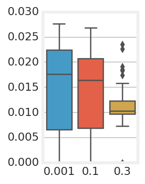
There are two sets of parameters to initialize: the set of weights and the variational parameters of the rank-1 distributions and . The weights are initialized just as in deterministic networks. For the variational posterior distributions, we initialize the mean following BatchEnsemble: random sign flips of or a draw from a normal centered at 1. This encourages each sampled vector to be roughly orthogonal from one another (thus inducing different directions for diverse solutions as one takes gradient steps); unit mean encourages the identity.
For the variational standard deviation parameters , we explore two approaches (Figure 8). The first is a “deterministic initialization,” where is set close to zero such that—when combined with KL annealing—the initial optimization trajectory resembles a deterministic network’s. This is commonly used for variational inference (e.g., Kucukelbir et al. 2017). Though this aids optimization and aims to prevent underfitting, one potential reason for why BNNs still underperform is that a deterministic initialization encourages poorly estimated uncertainties: the distribution of weights may be less prone to expand as the annealed KL penalizes deviations from the prior (the cost tradeoff under the likelihood may be too high). Alternatively, we also try a “dropout initialization”, where standard deviations are reparameterized with a dropout rate: where is the binary dropout probability.33 3 To derive this, observe that dropout’s Bernoulli noise, which takes the value with probability and otherwise, has mean and variance (Srivastava et al. 2014). Dropout rates between 0.1 and 0.3 (common in modern architectures) imply a standard deviation of 0.3-0.65. Figure 8 shows accuracy and calibration both decrease as a function of initialized dropout rate; NLL stays roughly the same. We recommend deterministic initialization as the accuracy gains justify the minor cost in calibration.
C.2 Real-valued Scale Parameterization
As shown in Equation 3, the hierarchical prior over and induces a prior over the scale parameters of the layer’s weights. A natural question that arises is: should the and priors be constrained to be positive-valued, or left unconstrained as real-valued priors? Intuitively, real-valued priors are preferable because they can modulate the sign of the layer’s inputs and outputs. To determine whether this is beneficial and necessary, we perform an ablation under our CIFAR-10 setup (Section 4). In this experiment, we compare a global mixture of Gaussians for the real-valued prior, and a global mixture of log-Gaussian distributions for the positive-valued prior. For each, we tune over the initialization of the prior’s standard deviation, and the L2 regularization for the point-wise estimated . For the Gaussians, we also tune over the initialization of the prior’s mean.
Figure 9 displays our findings. Similar to study of priors over , , or both, we compare results across NLL, accuracy, and ECE on the test set and CIFAR-10-C corruptions dataset. We find that both setups are comparable on test accuracy, and that the real-valued setup outperforms the other on test NLL and ECE. For the corruptions task, the two setups compare equally on NLL, and differ on accuracy and ECE.

C.3 Number of Evaluation Samples
In Table 8, we experiment with using multiple weight samples, per mixture component, per example, at evaluation time for our Wide ResNet-28-10 model trained on CIFAR-10. In all cases, we use the same model that was trained using only a single weight sample (per mixture component, per example). As expected, an increased number of samples improves metric performance, with a significant improvement across all corrupted metrics. This demonstrates one of the benefits to incorporating local distributions over each mixture component, namely that given an increased computational budget, one can improve upon the metric performance at prediction time.
| Method | NLL() | Accuracy() | ECE() | cNLL / cA / cECE | |
| Rank-1 BNN - Gaussian | 1 sample | 0.128 | 96.3 | 0.008 | 0.84 / 76.7 / 0.080 |
| 4 samples | 0.126 | 96.3 | 0.008 | 0.80 / 77.3 / 0.074 | |
| 25 samples | 0.125 | 96.3 | 0.007 | 0.77 / 77.8 / 0.070 | |
| Rank-1 BNN - Cauchy | 4 samples | 0.120 | 96.5 | 0.009 | 0.74 / 80.5 / 0.090 |
| Deep Ensembles | WRN-28-5 | 0.115 | 96.3 | 0.008 | 0.84 / 77.2 / 0.089 |
| WRN-28-10 | 0.114 | 96.6 | 0.010 | 0.81 / 77.9 / 0.087 | |
Appendix D Additional Discussion and Future Directions
For future work, we’d like to push further on our results by scaling to larger ImageNet models to achieve state-of-the-art in test accuracy alongside other metrics. Although we focus on variational inference in this paper, applying this parameterization in MCMC is a promising parameter-efficient strategy for scalable BNNs. As an alternative to using mixtures trained with the average per-component log-likelihood, one can use multiple independent chains over the rank-1 factors. Another direction for future work is the straightforward extension to higher rank factors. However, prior work (Swiatkowski et al. 2019; Izmailov et al. 2019) has demonstrated diminishing returns that practically stop at ranks 3 or 5.
One surprising finding in our experimental results is that heavy-tailed priors, on a low-dimensional subspace, can significantly improve robustness and uncertainty calibration while maintaining or improving accuracy. This is likely due to the heavier tails allowing for more points in loss landscape valleys to be covered, whereas a mixture of lighter tails could place multiple modes that are nearly identical. However, with deeper or recurrent architectures, samples from the heavy-tailed posteriors seem to affect the stability of the training dynamics, leading to slightly worse predictive performance. One additional direction for future work is to explore ways to stabilize automatic differentiation through such approximate posteriors or to pair heavy-tailed priors with sub-Gaussian posteriors.
Appendix E Choices of Loss Functions
E.1 Definitions
E.2 Negative log-likelihood of marginalized logits
| (11) |
E.3 Negative log-likelihood of marginalized probs
| (12) |
E.4 Marginal Negative log-likelihood (i.e., average NLL or Gibbs cross-entropy)
| (13) |
E.5 Negative log marginal likelihood (i.e., mixture NLL)
| (14) |
As we saw in Section 3, due to Jensen’s inequality, (14) (13). However, we find that minimizing the upper bound (i.e. Eq. 13) to be easier while allowing for improved generalization performance. Note that for classification problems (i.e., Bernoulli or Categorical predictive distributions), Eq. 12 is equivalent to Eq. 14, though more generally, marginalizing the parameters of the predictive distribution before computing the negative log likelihood (Eq. 12) is different from marginalizing the likelihood before taking the negative log (Eq. 14), and from marginalizing the negative log likelihood (Eq. 13). Also note that though they are mathematically equivalent for classification, the formulation of Eq. 14 is more numerically stable than Eq. 12.
Appendix F Out-of-distribution Performance
F.1 CIFAR-10-C Results


F.2 CIFAR-100-C Results


F.3 ImageNet-C Results


