PENNI: Pruned Kernel Sharing for Efficient CNN Inference
Abstract
Although state-of-the-art (SOTA) CNNs achieve outstanding performance on various tasks, their high computation demand and massive number of parameters make it difficult to deploy these SOTA CNNs onto resource-constrained devices. Previous works on CNN acceleration utilize low-rank approximation of the original convolution layers to reduce computation cost. However, these methods are very difficult to conduct upon sparse models, which limits execution speedup since redundancies within the CNN model are not fully exploited. We argue that kernel granularity decomposition can be conducted with low-rank assumption while exploiting the redundancy within the remaining compact coefficients. Based on this observation, we propose PENNI, a CNN model compression framework that is able to achieve model compactness and hardware efficiency simultaneously by (1) implementing kernel sharing in convolution layers via a small number of basis kernels and (2) alternately adjusting bases and coefficients with sparse constraints. Experiments show that we can prune 97% parameters and 92% FLOPs on ResNet18 CIFAR10 with no accuracy loss, and achieve 44% reduction in run-time memory consumption and a 53% reduction in inference latency.
Keywords:
Network Pruning, Model Compression and Acceleration, CNN1 Introduction
One of the greatest strengths of Deep Neural Networks (DNNs), specifically Convolutional Neural Networks (CNNs), is their large design space, which innately heightens flexibility and potential for accuracy. Improving model accuracy conventionally involves increasing its size, given sufficient training data. This increase in size can come in the form of more layers (He et al. 2016), more channels per layer (Zagoruyko & Komodakis 2016), or more branches (Szegedy et al. 2015). A major drawback of naïvely increasing model size is the substantial computational power and memory bandwidth required to train and run inference tasks. To address this issue, multiple methods have been introduced to compress CNN models and increase sparsity (Han et al. 2015; Wen et al. 2016). Model compression can come in the form of weight quantization (Ullrich et al. 2017) or Low Rank Approximation (LRA) (Denton et al. 2014).
LRA utilizes matrix factorization to decompose weight matrices into the product of two low rank matrices, thus reducing computation cost. Some works (Lebedev et al. 2014; Tai et al. 2016) use tensor decomposition to represent the original weight with the outer product of one-dimensional tensors (i.e., vectors) . The speedup and parameter reduction of these methods are notable; however, current approaches are limited because they do not consider redundancies in CNN parameters.
Model sparsity can be induced via various pruning techniques, most of which are categorized under structured or unstructured. On one hand, unstructured pruning aims to remove unimportant weights of a network, irrespective of its location. By targeting the least important weights in a model, unstructured pruning has minimal impact on overall accuracy while achieving a high sparsity level. However, the undefined distribution of pruned weights makes it challenging to compress the model’s representation in memory. On the other hand, structured pruning achieves sparsity by removing entire DNN structures (e.g. filter-channels, filters, layers, etc.) that are deemed unimportant, which may impact a model’s performance by inadvertently removing sensitive parameters. Such predictable pruning patterns open the avenue for efficient model storage and computation. It is important to note that merely applying structured pruning is not enough to fully reap hardware efficiency benefits. Without additional changes to the underlying representation in memory or the model’s training or inference stage algorithms, conventional DNN platforms still fall victim to inefficient memory transfers and computations.
In this paper, we propose Pruned kernel sharing for Efficient CNN Inference (PENNI), a CNN model compression framework that overcomes these challenges by decomposing layer parameters into tiny sets of basis kernels and accompanying coefficient matrices. This method can benefit inference efficiency by organizing the involved coefficients and computation flow in a hardware-friendly manner. High compression rate is achieved by applying -regularization to the coefficients. The structural redundancies are further explored in a model shrinkage procedure. We evaluate our method on CIFAR10 and ImageNet with VGG16, ResNet and AlexNet. Results show that we can achieve a 98.3% reduction on parameters and a 93.3% reduction on FLOPs with less than 0.4% accuracy drop. PENNI outperforms state-of-the-art (SOTA) pruning schemes in addition to being more efficient for hardware implementation. Our code is avaliable at: https://github.com/timlee0212/PENNI.
Our main contributions are listed as follows:
- •
We propose a hardware-friendly CNN model compression framework, PENNI. We apply filter decomposition to generate a limited set of basis kernels and corresponding coefficient matrix. Sparsity is achieved by applying -regularization to coefficient matrices in the retraining process. Structural redundancies are then explored via a model shrinking procedure.
- •
Hardware inference efficiency is directly benefited through model shrinking with no modifications to inference algorithm. Further speedup can be brought by computation reorganization of convolutional layers. To avoid restoring original filter tensors, we can separate basis kernel convolutions from their weighted sum computation. Keeping the two computation steps distinct opens the avenue for exposing all pruned coefficients, thus leveraging coefficient sparsity and avoiding wasteful zero-computations.
- •
Evaluation on CIFAR-10 and ImageNet with various network architectures proves the effectiveness of the proposed method with significant reduction in both FLOPs and number of parameters with negligible accuracy loss.
2 Related Work
Various methods have been proposed to accelerate CNN inference. These methods either exploit redundancies of CNN models to reduce the number of parameters and computations or introduce lightweight model structures for a given task.
Compact Model Design
Previous works aim to develop resource-efficient model structures to reduce computation requirements and improve latency. Lin et al. (Lin et al. 2013) propose global average pooling and 1x1 convolution, which are widely adopted in the later compact architectures. SqueezeNet (Iandola et al. 2016) utilizes both structures to reduce the number of channels and remove fully-connected layers. A similar idea appears in InceptionNet (Szegedy et al. 2015), while a later version (Szegedy et al. 2016) extends the idea by spatially separating the convolutional layers. MobileNet (Howard et al. 2017) uses depthwise separable convolution to reduce the computation cost by splitting the original convolutional layer channel-wise. Its following version, MobileNet V2 (Sandler et al. 2018), adopts residual connections and introduces the inverted bottleneck module to improve efficiency. Xie et al. (Xie et al. 2017) enhance the expressiveness of the depthwise convolution by allowing limited connectivity within groups, while later ShuffleNet (Zhang et al. 2018b) adopts the grouped convolution. In addition to the manually designed compact architectures listed above, Neural Architecture Search (NAS) methods aim to automatically find architectures with optimal balances of compactness and performance. Multiple such works (Tan et al. 2019; Cai et al. 2019; Liu et al. 2019a; Tan & Le 2019) generate architectures that outperform manually designed ones.
Low Rank Approximation
Low Rank Approximation (LRA) method decomposes the original weights into several low rank matrices (Denton et al. 2014; Zhang et al. 2015) or low dimension tensors (Lebedev et al. 2014; Kim et al. 2015). Denton et al. (Denton et al. 2014) utilize Singular Value Decomposition (SVD) to conduct the decomposition, whereas Zhang et al. (Zhang et al. 2015) take nonlinear activations into account to obtain the decomposition while minimizing error of the response. Kim et al. (Kim et al. 2015) adopt Tucker Decomposition to compress the kernel tensor. Lebedev et al. (Lebedev et al. 2014) use canonical polyadic (CP) decomposition. In addition, Learning Structured Sparsity (Wen et al. 2016) and Centripetal-SGD (Ding et al. 2019a) directly train the DNN with low rank constraints. These tensor decomposition methods rely on the rank selection, which is an ill-posed problem, while the matrix factorization methods have limited speedup since redundancies in the standalone weight values are not considered.
Model Pruning
The idea of weight pruning dates back to the last century. Optimal Brain Damage (LeCun et al. 1990) proposes pruning weight based on their impact on the loss function. A later work, Optimal Brain Surgeon (Hassibi & Stork 1993) improves this method by replacing the diagonal Hessian Matrix with an approximated full covariance matrix. However, due to the giant size of the modern DNNs, these methods incur unacceptable computation cost. Han et al. (Han et al. 2015) propose pruning weights by comparing the magnitude with a threshold, and achieve the optimal result by iterative pruning and fine-tuning. Guo et al. (Guo et al. 2016) further improve the sparsity level by maintaining a mask instead of directly pruning the redundant weights. Beyond conventional unstructured pruning methods, various structured pruning methodologies have been proposed to ease translation from sparsity to inference speedup. Wen et al. (Wen et al. 2016) and Yang et al. (Yang et al. 2019) apply group regularizer in the training process to obtain structured sparsity. Liu et al. (Liu et al. 2017) apply -regularization to the scaling factors of batch normalization layers to identify insignificant channels. ThiNet (Luo et al. 2017) utilizes a data-driven method to prune the channel with the smallest impact on the following layer. In recent works (He et al. 2018a; Zhang et al. 2018a; He et al. 2019; Ding et al. 2019b), different criteria are adopted to rank the importance of the filter. Louizos et al. (Louizos et al. 2017) use stochastic gates to apply -regularization to the filters. NAS methods also incorporate filter pruning (He et al. 2018b; Liu et al. 2019b). Although structured pruning can directly benefit the inference efficiency, its pruning granularity limits the compression rate or accuracy of CNN models.
3 Proposed Method
3.1 Overview
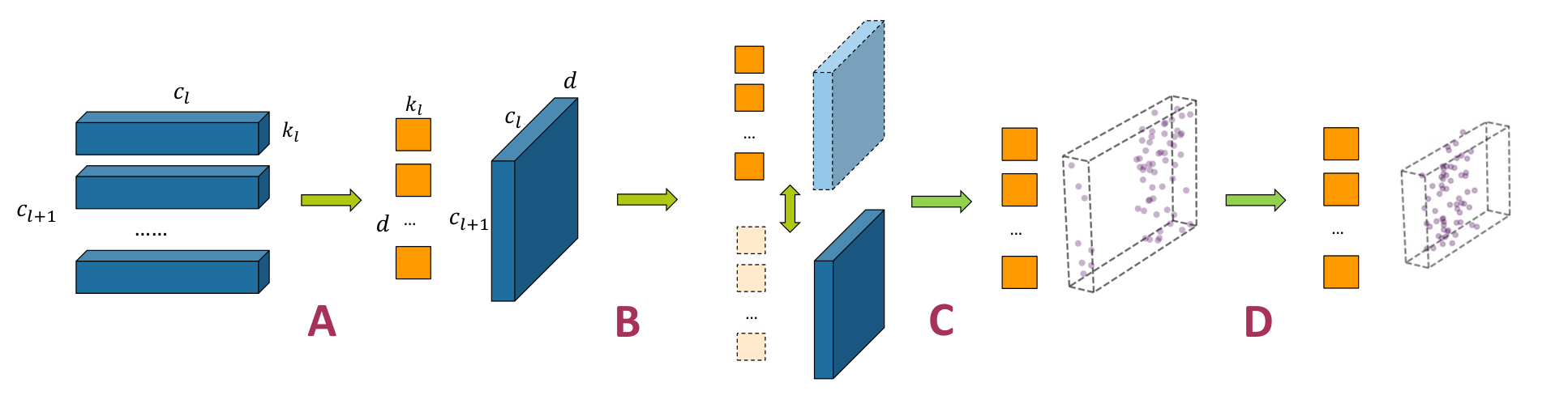
Fig.1 presents the overview of PENNI framework. We first decompose each layer’s convolution filters into a few basis kernels and a coefficient matrix. Then, we retrain the decomposed network with sparsity regularization applied to coefficient matrix to recover any lost accuracy. Finally, we prune the redundant coefficients based on magnitude and obtain a compact CNN model.
Before the discussion on the method, we first define the notations that will be used in this paper. We denote the parameters of convolutional layer as , where is the number of the input channels, is the number of the output channels, and and are the kernel dimensions. Since most CNN architectures implement a square kernel shape, i.e., , we denote the kernel shape as for simplicity; the shape of the kernel does not affect this framework. is the set of all parameters of convolutional layers of a CNN model. We denote the output features of layer as , and the input features as . represents the data pairs, while is the given label or unknown ground-truth. represents the network model’s prediction. With these notations, the -th channel of a layer’s output feature map can be computed by:
| (1) |
where is the -th kernel of the -th filter, is the bias term of the -th filter and the is the non-linear function of the layer .
3.2 Filter Decomposition
The convolution operation dominates computation cost of CNN inference. Irregular data access and compute patterns make it extremely difficult to efficiently map the operation onto parallel hardware and further improve inference efficiency. We address this issue by reducing the number of convolution operations and offloading the irregular computation to a sequential and simple pattern.
Previous work (Zhang et al. 2015) on accelerating CNN inference utilizes a low rank assumption of output feature subspace to represent the original weight matrix with the multiplication of two low rank matrices, thus reducing the computation required. Low rank assumption is reasonable in this case because the number of output features is comparable with the dimension of the feature space. Recent work (Ding et al. 2019a) indicates that in most CNNs, regularization on convolutional kernels can push the kernels to be alike one another. Based on this observation, we argue that the low rank assumption can also be applied to the subspace that each convolutional kernel lies in. With this assumption, we approximate the original convolutional layer by sharing a tiny set of basis kernels and representing original kernels with coefficients.
Decomposition at a kernel granularity is done to obtain an approximated layer. This process applies to a single layer a time, so the superscript is omitted for readability. We first reshape the original weight tensor into a 2D matrix ; thus, each kernel can be seen as its row vector . Suppose is a subspace with basis where . The objective of decomposition process is to find the subspace that minimizes the error between the projected and original vectors, shown in Equation 2.
| (2) |
is the basis matrix where each column vector is a basis of the subspace and is the coefficient vector corresponding to the row vector . With this decomposition, the output of each layer is computed by:
| (3) |
where is the row vector in the coefficient matrix corresponding to the -th kernel of the -th filter.
The decomposition problem can be formulated as best approximation and is perfectly solved using singular value decomposition (SVD). We first obtain by subtracting each row vector with the mean vector, and then compute the covariance matrix . Conducting SVD on , and organizing the singular value by their magnitude, we’ll have:
| (4) |
The basis matrix is then derived by selecting the first columns from matrix and obtaining the corresponding coefficients by multiplying the by the projection matrix . Normally, and parameter matrices of a pretrained model are dense, so is a full rank matrix with the rank . Thus, the low rank approximation on kernel space makes the SVD computation faster than conducting decomposition at the filter granularity. A singular value may represent the portion of the basis vector contributing to the original vectors; but, rather than selecting based on it, we leave it as a hyper-parameter providing a trade-off between computational cost and model accuracy.
3.3 Retraining
Although the discussed filter decomposition scheme gives the best approximation of the original parameters in low-rank subspace, the model accuracy may greatly degrade due to varying sensitivity of affected weights. Zhang et al. (Zhang et al. 2015) address this issue by considering the non-linear block and minimizing response of the layer. However, innate redundancies in the models are not exploited, which limits the compression rate and the speedup. Thus, we incorporate a retraining process for twofold benefits: recover the model accuracy and exploit redundancy within the CNN structure through coefficient sparsity regularization. The objective of retraining phase is to minimize the loss:
| (5) |
where the first term is the original loss of the model (i.e., cross entropy loss), the second term is the sum of the coefficients magnitude and is the strength of the sparsity regularization.
If we visualize these two parameter sets as separate layers, it conceptually increases the depth of the model and makes it harder to converge. Thus, in the training process, we generate the reconstructed parameter from the basis and coefficients and compute the gradients as the original convolutional layer. The chain rule can then be applied to derive the gradients of the basis and the coefficients from the original convolutional layer’s gradients. Specifically,
| (6) |
where the and is the coefficient matrix. Again, we omit the superscript for readability.
The gradient of coefficient matrix consists of two terms. The first term pushes the coefficient towards the direction that decreases the error, while the second term coerces the reconstructed kernels to be close to the basis kernels. If we jointly train the basis and coefficients, the coefficients will be updated based on the old basis and vice versa. Jointly training both makes it very difficult for the model to converge, producing further accuracy drop. We avoid this issue by conducting retraining in an alternating fashion, i.e., freezing the coefficients and train the basis for several epochs and then freezing the basis and train coefficients.
The decomposed manner can also benefit the sparsity regularization. Since -regularizer is non-smooth, it equates to adding a constant to the gradient, which dominates the gradient in the later stage of training. This causes the training process to be very unstable or unable to converge. Regularization on the decomposed filter state avoids this issue. Examining the gradient from the original weight’s perspective, the regularization constant is essentially scaled as a consequence of being applied only to the coefficients. This scaling factor decreases the constant proportional to the diminishing gradients. The constant is still within the same magnitude of the gradient of the loss term, thus stabilizing the process of converging to a sparse parameter set.
3.4 Model Shrinking
Retraining the filter-decomposed model with sparsity regularization results in predominantly near-zero coefficients. As shown in (Han et al. 2015), we can select a threshold based on the standard deviation of each coefficient matrix and prune all weight values with a magnitude lower than the threshold. Only a few epochs of coefficient fine-tuning is required to recover accuracy lost by pruning. A combination of high sparsity level and low accuracy loss can be achieved without any additional iterations.

The sparse coefficients expose redundancies in CNN structures that can be utilized to shrink the model. Model shrinkage begins with reshaping the coefficient matrix into the shape . By selecting the first dimension (i.e., the input channels) and summing the number of the non-zero elements of the remaining two dimensions, we can obtain a vector with elements. Zeros in indicate that corresponding input channels are redundant since no output channels are connected. Indices of these channels can be represented by the set . Selecting the second dimension (i.e., the output channels) and conducting the same procedure, we can get and , which indicate redundant output channels. The redundancies in basis kernels can also be derived with the same procedure.
Note that it is possible for redundancies of a layer’s input and output channels to not match. We can exploit this feature by considering the connections between input channels and redundant output channels of the same layer. If some input channels only have connections to redundant output channels, these inputs consequentially become redundant. Thus, we iteratively update the redundancy sets by applying the following steps. First, we take the union of the current layer’s output channels with the next layer’s input channels, i.e., . Then, we update by setting all corresponding coefficients in and to zero and deriving new redundancy vectors and sets. This procedure, depicted in Fig. 2, is repeated until no modification is made in an iteration.
A potential problem with the iterative update procedure is when it is applied to CNN architectures with skip connections, such as ResNet (He et al. 2016). Specifically, dimensions of pruned output feature maps might be inconsistent with corresponding skip connections. The solution to this issue is straightforward. If the shortcut path has a dimension-matching operation (i.e., 11 convolution), we update the output channel of the 11 convolution and the current layer by taking the intersection of their redundancy sets. If the shortcut path has no such operation, we will need to update the redundancy sets of the start and the end of the skip connection before updating the coefficients.


3.5 Hardware Benefit
The decisive advantage of PENNI over previous CNN pruning, compression, or filter decomposition methods is its potential for synergistic reduction of memory and computational footprints. PENNI directly leverages filter decomposition by enabling a partition of the convolution step into two distinct stages.
The first stage involves channel-by-channel convolutions with each of the two-dimensional basis kernels, producing intermediate feature maps; this stage is analogous to to depthwise separable convolution (Chollet 2017) with branches. Each branch duplicates one of the basis kernels across the input channels. Applying such a technique greatly reduces the number of multiply-and-accumulates (MACs) in the convolution step, which is the bottleneck in convolutional layers.
The second stage is a weighted sum to produce the convolutional layer’s output feature map. Specifically, intermediate feature maps are multiplied element-wise with the coefficient matrix and then accumulated at the output. As described in Section 3.4, the coefficient matrices are incredibly sparse; therefore, we reduce the model’s memory footprint and prevent redundant zero-multiply computations by representing the coefficients through a sparse matrix format. Although this stage introduces additional computations that offset the reduction in MACs from the first stage, the overall number of computations is dramatically reduced, thus improving inference latency.
Beyond the aforementioned straightforward benefits of the proposed two-stage convolutional layer scheme, PENNI also offers a unique attribute that can be leveraged for current and future hardware accelerator designs. The deterministic convolutional kernel structure means that the number of basis kernels can be altered to fit nicely with the number of processing elements (PEs) in accelerators such as DaDianNao (Chen et al. 2014) without forcing the model to conform to the hardware (e.g. reducing layer width). Meanwhile, the weighted sum stage can be computed in a streaming manner, much favored by single-instruction, multiple-data (SIMD) processors. Also, because data access patterns of convolutional layers conventionally require hardware-specific data-reuse algorithms to minimize costly cache evictions, removing interactions of the input channels at the convolution step via depthwise separation alleviates hardware complexity. Lastly, partitioning the convolution step to two stages opens the avenue for further accelerator-based throughput optimizations such as pipelining.
| Arch | Method | Base Acc. | Pruned Acc. | Param. | FLOPs | |||
|---|---|---|---|---|---|---|---|---|
| VGG16 | Baseline | 93.49% | - | - | 14.71M | - | 314.26M | - |
| PFEC | 93.25% | 93.40% | -0.15% | 5.4M | 64% | 206M | 34.2% | |
| Slimming | 93.62% | 93.56% | -0.06% | 1.77M | 87.97% | 127M | 43.50% | |
| AOFP | 93.38% | 93.28% | -0.10% | - | - | 77M | 75.27% | |
| Ours-D | 93.49% | 93.14% | -0.35% | 183.4M | 44.44% | 183.4M | 41.65% | |
| Ours-P | 93.49% | 93.12% | -0.37% | 0.135M | 98.33% | 21.19M | 93.26% | |
| ResNet18 | Baseline | 93.77% | - | - | 11.16M | - | 555.43M | - |
| Ours-D | 93.77% | 93.89% | +0.12% | 6.28M | 56.27% | 332.34M | 40.17% | |
| Ours-P | 93.77% | 94.01% | +0.24% | 0.341M | 96.94% | 44.98M | 91.90% | |
| ResNet56 | Baseline | 93.57% | - | - | 0.848M | - | 125.49M | - |
| PFEC | 93.04% | 93.06% | +0.02% | 0.73M | 13.7% | 90.9M | 27.6% | |
| SFP | 93.59% | 93.35% | -0.24% | - | - | 59.4M | 52.67% | |
| C-SGD | 93.39% | 93.44% | +0.05% | - | - | - | 60.85% | |
| FPGM | 93.59% | 93.49% | -0.10% | - | - | 59.4M | 52.67% | |
| Group-HS | 93.14% | 93.45% | +0.31% | - | - | - | 68.43% | |
| Ours-D | 93.57% | 94.00% | +0.43% | 0.471M | 44.46% | 92.80M | 26.15% | |
| Ours-P | 93.57% | 93.38% | -0.19% | 39.37K | 95.36% | 28.98M | 79.40% |
4 Experiments
In this section, we demonstrate the effectiveness of the proposed framework. Experiments were held on CIFAR10 (Krizhevsky et al. 2009) and ImageNet (Deng et al. 2009) datasets. Experiment settings are detailed before comparing compression results between PENNI and both state-of-the-art channel pruning and weight pruning methods. Finally, we conduct an ablation study to show the contribution of each component in the framework.
4.1 Experiment Settings
CIFAR10
On CIFAR-10, we chose VGG16 (Simonyan & Zisserman 2014), ResNet18 and ResNet56 (He et al. 2016) for experimentation. VGG16 is a small version tailored for CIFAR10. We use ResNet56 to test the performance on compact models. Model training involved the following data preprocessing steps: random flipping, random cropping with 4 pixels padding, and normalization. The VGG16 and ResNet18 models were first pretrained for 100 epochs with 0.1 initial learning rate; then, the learning rate was multiplied by 0.1 at 50% and 75% epochs, while ResNet56 was pretrained for 250 epochs with the same learning rate scheduling. All pretraining, retraining and fine-tuning procedures implemented Stochastic Gradient Descent (SGD) as the optimizer with weight decay, 0.9 momentum, and batch size set to 128. We selected for the decomposition stage and retrained for 100 epochs with 0.01 initial learning rate and the same scheduling. Regularization strength was set to . The interval between training basis and coefficients was set to 5 epochs. The final fine-tuning procedure took 30 epochs with 0.01 initial learning rate and the same scheduling scheme.
ImageNet
On ImageNet, we used AlexNet (Krizhevsky et al. 2012) and ResNet50 for the experiment, incorporating the pretrained models provided by PyTorch (PyTorch 2019). Since AlexNet has different kernel sizes across layers, we selected and for the first two convolutional layers, and for the rest 33 convolutional layers. For ResNet50, we use 4 sets of parameter settings, with and regularization strength set to and . The retraining procedure lasted 50 epochs with the same hyper-parameters as CIFAR10 but set batch size to 256 and cosine annealing. For AlexNet, we warmed up with a learning rate of for five epochs; then, the learning rate was set to for the remaining 45 epochs. The fine-tune procedure took 30 epochs with learning rate set to 0.01 for ResNet50 and 0.0001 for AlexNet.
4.2 CIFAR10 Results
We selected channel pruning methods PFEC (Li et al. 2016), Slimming (Liu et al. 2017), SFP (He et al. 2018a), AOFP (Ding et al. 2019b), C-SGD (Ding et al. 2019a), FPGM (He et al. 2019) and Group-HoyerSquare (Yang et al. 2019) for comparison. For the works providing parameter trade-offs, we use results with similar accuracy drop. The results are shown in Table 1. ‘Ours-D’ denotes the compression result with only decomposition and retraining phases, while ‘Ours-P’ incorporates all four phases. We only consider the parameters of the convolutional and linear layers, and the FLOP count is taken by calculating the number of Multiply-Accumulation (MAC) operations. Based on the computation flow described in Section 3.5, we consider that the sparsity of coefficient matrix can be converted to reduction in FLOPs. Thus, we ignore the zeros in the coefficient matrices when counting FLOPs. On VGG16, we outperformed channel pruning methods by achieving a reduction over 98% on parameters and 93.26% on FLOPs. Although there is a slightly higher accuracy drop, it is only 0.15% behind AOFP with 10% extra reduction on FLOPs and 0.42% behind Slimming with almost double reduction on FLOPs, which is acceptable. Since ResNet18 is originally designed for the ImageNet dataset, no previous work has provided result for comparison. We include it in this paper to show that PENNI is able to shrink over-parameterized models and may improve accuracy. On ResNet56, which is a compact model specially tailored for CIFAR10, we can still prune 94.52% parameters and 76.9% FLOPS with 0.2% accuracy drop. Our method outperformed previous channel pruning methods by a nearly 20% extra FLOPs reduction, and a 10% extra reduction over the group regularization method.
4.3 ImageNet Results
| Method | Top-1 | Top-5 | FLOPs | |
|---|---|---|---|---|
| Baseline | 56.51% | 79.07% | 773M | - |
| AOFP | 56.17% | 79.53% | 492M | 41.33% |
| Ours-D | 55.41% | 78.30% | 573M | 25.88% |
| Ours-P | 55.57% | 78.32% | 232M | 70.04% |
| Method | Top-1 | Top-5 | FLOPs | |
| Baseline | 76.13% | 92.86% | 4.09G | - |
| Ours-D | 76.20% | 92.85% | 3.23G | 21.10% |
| ThiNet-70 | 72.02% | 90.67% | 2.58G11 1 Computed based on the reduction percentage reported by original paper. | 36.80% |
| Ours-R1 | 73.87% | 91.79% | 220M | 94.73% |
| SFP | 74.61% | 92.06% | 2.38G1 | 41.80% |
| C-SGD-50 | 74.54% | 92.09% | 1.81G1 | 55.76% |
| Ours-R2 | 74.74% | 92.27% | 527M | 87.12% |
| C-SGD-60 | 74.93% | 92.27% | 2.20G1 | 46.24% |
| FPGM-40% | 74.83% | 92.32% | 1.90G1 | 53.50% |
| Ours-R3 | 75.00% | 92.21% | 576M | 85.92% |
| AOFP-C1 | 75.63% | 92.69% | 2.58G | 32.88% |
| AOFP-C2 | 75.11% | 92.28% | 1.66G | 56.73% |
| C-SGD-70 | 75.27% | 92.46% | 2.59G1 | 36.75% |
| FPGM-30% | 75.59% | 92.63% | 2.36G1 | 42.20% |
| Ours-R4 | 75.66% | 92.79% | 768M | 81.23% |
On ImageNet, we chose Slimming, ThiNet (Luo et al. 2017), SFP, AOFP, C-SGD and FPGM for comparison. The result of AlexNet compression is shown in Table 2. We can prune 70.04% FLOPs with 1% loss on top-1 accuracy. For ResNet50, we observe the 11 convolutional layer of the bottleneck block as the coefficient matrix with 1-D basis and apply regularization to it. Table 3 shows the result on ResNet50 compression. We use multiple parameter settings to justify the trade-off between accuracy and compression rate. ‘Ours-D’ only involves decomposition and retraining step with , while ‘R1’ and ‘R2’ incorprate pruning and shrinking phases with regularization strength set to and . ‘R3’ and ‘R4’ has the same parameter apart from setting in the decomposition phase. The results show that the decomposition step can reduce more than 20% of the FLOPs with no accuracy drop. With the pruning and shrinking procedures, 94.73% of the FLOPS can be pruned with 2.4% top-1 accuracy loss. When we relax the regularization, we can still prune 81.23% of the FLOPs with only 0.5% accuracy loss. The FLOPs reduction is nearly two times the reduction of previous channel pruning methods. A even larger compression rate can be achieved by combining the 11 convolutional layer with the coefficient matrices.
4.4 Inference Acceleration
| Device | Variation | Latency(ms) | Memory(MB) |
|---|---|---|---|
| CPU | Baseline | 12.9 | 137 |
| PENNI | 5.96 | 77.6 | |
| GPU | Baseline | 10.8 | 487 |
| PENNI | 7.26 | 424 |
Hardware Settings
We used Intel Xeon Gold 6136 to test the inference performance for CPU platform and NVIDIA Titan X for the GPU platform. For software, we used PyTorch 1.4 (Paszke et al. 2019) to implement the inference test. Batch size was set to 128 (1) for inference testing on the GPU (CPU). GPU inference batch size is higher than CPU to increase utilization and emphasize the latency impact of our method on the highly parallel platform. We indicate these settings as latency and peak memory consumption values vary across platforms or library versions.
Table 4 displays inference latencies and memory consumption recorded for the baseline and PENNI framework. As mentioned in 3.5, one of PENNI’s defining strengths is its impact on computational and memory footprints. Results shown in Table 4 reveal a 1.5 (2.2) reduction in measured inference latency on the GPU (CPU). Peak memory consumption also benefited from a 1.1 (1.8) reduction. It is important to note that these metrics were taken without applying the convolution computation reorganization described in 3.5; this is done intentionally to reveal the effectiveness of our model shrinkage with zero changes to the hardware and inference-time computation. The reduction in memory is a straightforward consequence of the decomposition and shrinking stages of the PENNI framework. Although our method is successful at dramatically decreasing model size in memory, intermediate feature maps seems to dominate on-device memory consumption, especially with a batch size of 128 on the GPU.
4.5 Subspace Dimension
To justify the selection of the parameter , we conduct an experiment with different decompose dimensions. We used the same VGG16 baseline model and hyper-parameters as 4.2. The result is shown in Fig.4 indicates that the remaining FLOPs scales linearly with the number of basis kernels. This is expected since the number of convolutional operations is determined by . The parameters scale linearly before 6-D basis and have minor difference with the increasing dimension. This is because even though more basis vector requires more coefficients, it also adds flexibility and thus leads to sparser coefficients. The test accuracy reveals the same trend, with , minor improvement on the accuracy can be brought by increasing . Thus, we select for the balance between parameter and FLOPs reduction and accuracy drops.
4.6 Model Shrinking
We show the effectiveness of model shrinking by comparing layer widths. As shown in Figure 5, on VGG16, the model shrinking procedure effectively removes redundant channels in the second half of all layers. Meanwhile, on ResNet56, the shrinking is limited by the dimension matching requirement of the skip connections. The oscillation pattern of the layer width indicates that redundancies of the inner-block layer can be effectively exploited. These results show that PENNI can benefit unmodified inference software and hardware by exploiting structural redundancies.
5 Conclusion
This work proposes the PENNI framework for hardware-friendly CNN model compression. Our method improves inference latency with no changes to inference algorithms and hardware via model shrinking, thus translating model sparsity to speedup. A low rank assumption is used to decompose CNN filters into basis kernels and prune the resulting coefficient matrices, which results in structured sparsity. A novel alternating fine-tuning method is used to further increase sparsity and improve model performance. Unique characteristics generated by the decomposition step may be leveraged for hardware efficiency via convolution computation reorganization, directly benefiting modern DNN platforms.
Acknowledgment
This work was supported in part by NSF-1937435, NSF-1822085, NSF-1725456, ARO W911NF-19-2-0107, and NSF IUCRC for ASIC memberships from Cadence etc.
References
- Cai et al. (2019) Cai, H., Zhu, L., and Han, S. ProxylessNAS: Direct neural architecture search on target task and hardware. In International Conference on Learning Representations, 2019. URL https://openreview.net/forum?id=HylVB3AqYm.
- Chen et al. (2014) Chen, Y., Luo, T., Liu, S., Zhang, S., He, L., Wang, J., Li, L., Chen, T., Xu, Z., Sun, N., et al. Dadiannao: A machine-learning supercomputer. In 2014 47th Annual IEEE/ACM International Symposium on Microarchitecture, pp. 609–622. IEEE, 2014.
- Chollet (2017) Chollet, F. Xception: Deep learning with depthwise separable convolutions. In Proceedings of the IEEE conference on computer vision and pattern recognition, pp. 1251–1258, 2017.
- Deng et al. (2009) Deng, J., Dong, W., Socher, R., Li, L.-J., Li, K., and Fei-Fei, L. Imagenet: A large-scale hierarchical image database. In 2009 IEEE conference on computer vision and pattern recognition, pp. 248–255. Ieee, 2009.
- Denton et al. (2014) Denton, E. L., Zaremba, W., Bruna, J., LeCun, Y., and Fergus, R. Exploiting linear structure within convolutional networks for efficient evaluation. In Advances in neural information processing systems, pp. 1269–1277, 2014.
- Ding et al. (2019a) Ding, X., Ding, G., Guo, Y., and Han, J. Centripetal sgd for pruning very deep convolutional networks with complicated structure. In Proceedings of the IEEE Conference on Computer Vision and Pattern Recognition, pp. 4943–4953, 2019a.
- Ding et al. (2019b) Ding, X., Ding, G., Guo, Y., Han, J., and Yan, C. Approximated oracle filter pruning for destructive cnn width optimization. In International Conference on Machine Learning, pp. 1607–1616, 2019b.
- Guo et al. (2016) Guo, Y., Yao, A., and Chen, Y. Dynamic network surgery for efficient dnns. In Advances in neural information processing systems, pp. 1379–1387, 2016.
- Han et al. (2015) Han, S., Mao, H., and Dally, W. J. Deep compression: Compressing deep neural networks with pruning, trained quantization and huffman coding. arXiv preprint arXiv:1510.00149, 2015.
- Hassibi & Stork (1993) Hassibi, B. and Stork, D. G. Second order derivatives for network pruning: Optimal brain surgeon. In Advances in neural information processing systems, pp. 164–171, 1993.
- He et al. (2016) He, K., Zhang, X., Ren, S., and Sun, J. Deep residual learning for image recognition. In Proceedings of the IEEE conference on computer vision and pattern recognition, pp. 770–778, 2016.
- He et al. (2018a) He, Y., Kang, G., Dong, X., Fu, Y., and Yang, Y. Soft filter pruning for accelerating deep convolutional neural networks. arXiv preprint arXiv:1808.06866, 2018a.
- He et al. (2018b) He, Y., Lin, J., Liu, Z., Wang, H., Li, L.-J., and Han, S. Amc: Automl for model compression and acceleration on mobile devices. In Proceedings of the European Conference on Computer Vision (ECCV), pp. 784–800, 2018b.
- He et al. (2019) He, Y., Liu, P., Wang, Z., Hu, Z., and Yang, Y. Filter pruning via geometric median for deep convolutional neural networks acceleration. In Proceedings of the IEEE Conference on Computer Vision and Pattern Recognition, pp. 4340–4349, 2019.
- Howard et al. (2017) Howard, A. G., Zhu, M., Chen, B., Kalenichenko, D., Wang, W., Weyand, T., Andreetto, M., and Adam, H. Mobilenets: Efficient convolutional neural networks for mobile vision applications. arXiv preprint arXiv:1704.04861, 2017.
- Iandola et al. (2016) Iandola, F. N., Han, S., Moskewicz, M. W., Ashraf, K., Dally, W. J., and Keutzer, K. Squeezenet: Alexnet-level accuracy with 50x fewer parameters and¡ 0.5 mb model size. arXiv preprint arXiv:1602.07360, 2016.
- Kim et al. (2015) Kim, Y.-D., Park, E., Yoo, S., Choi, T., Yang, L., and Shin, D. Compression of deep convolutional neural networks for fast and low power mobile applications. arXiv preprint arXiv:1511.06530, 2015.
- Krizhevsky et al. (2009) Krizhevsky, A., Hinton, G., et al. Learning multiple layers of features from tiny images. 2009.
- Krizhevsky et al. (2012) Krizhevsky, A., Sutskever, I., and Hinton, G. E. Imagenet classification with deep convolutional neural networks. In Advances in neural information processing systems, pp. 1097–1105, 2012.
- Lebedev et al. (2014) Lebedev, V., Ganin, Y., Rakhuba, M., Oseledets, I., and Lempitsky, V. Speeding-up convolutional neural networks using fine-tuned cp-decomposition. arXiv preprint arXiv:1412.6553, 2014.
- LeCun et al. (1990) LeCun, Y., Denker, J. S., and Solla, S. A. Optimal brain damage. In Advances in neural information processing systems, pp. 598–605, 1990.
- Li et al. (2016) Li, H., Kadav, A., Durdanovic, I., Samet, H., and Graf, H. P. Pruning filters for efficient convnets. arXiv preprint arXiv:1608.08710, 2016.
- Lin et al. (2013) Lin, M., Chen, Q., and Yan, S. Network in network. arXiv preprint arXiv:1312.4400, 2013.
- Liu et al. (2019a) Liu, H., Simonyan, K., and Yang, Y. DARTS: Differentiable architecture search. In International Conference on Learning Representations, 2019a. URL https://openreview.net/forum?id=S1eYHoC5FX.
- Liu et al. (2017) Liu, Z., Li, J., Shen, Z., Huang, G., Yan, S., and Zhang, C. Learning efficient convolutional networks through network slimming. In Proceedings of the IEEE International Conference on Computer Vision, pp. 2736–2744, 2017.
- Liu et al. (2019b) Liu, Z., Mu, H., Zhang, X., Guo, Z., Yang, X., Cheng, K.-T., and Sun, J. Metapruning: Meta learning for automatic neural network channel pruning. In Proceedings of the IEEE International Conference on Computer Vision, pp. 3296–3305, 2019b.
- Louizos et al. (2017) Louizos, C., Welling, M., and Kingma, D. P. Learning sparse neural networks through regularization. arXiv preprint arXiv:1712.01312, 2017.
- Luo et al. (2017) Luo, J.-H., Wu, J., and Lin, W. Thinet: A filter level pruning method for deep neural network compression. In Proceedings of the IEEE international conference on computer vision, pp. 5058–5066, 2017.
- Paszke et al. (2019) Paszke, A., Gross, S., Massa, F., Lerer, A., Bradbury, J., Chanan, G., Killeen, T., Lin, Z., Gimelshein, N., Antiga, L., et al. Pytorch: An imperative style, high-performance deep learning library. In Advances in Neural Information Processing Systems, pp. 8024–8035, 2019.
- PyTorch (2019) PyTorch. Torchvision models, 2019. URL https://github.com/pytorch/vision/tree/master/torchvision/models.
- Sandler et al. (2018) Sandler, M., Howard, A., Zhu, M., Zhmoginov, A., and Chen, L.-C. Mobilenetv2: Inverted residuals and linear bottlenecks. In Proceedings of the IEEE conference on computer vision and pattern recognition, pp. 4510–4520, 2018.
- Simonyan & Zisserman (2014) Simonyan, K. and Zisserman, A. Very deep convolutional networks for large-scale image recognition. arXiv preprint arXiv:1409.1556, 2014.
- Szegedy et al. (2015) Szegedy, C., Liu, W., Jia, Y., Sermanet, P., Reed, S., Anguelov, D., Erhan, D., Vanhoucke, V., and Rabinovich, A. Going deeper with convolutions. In Proceedings of the IEEE conference on computer vision and pattern recognition, pp. 1–9, 2015.
- Szegedy et al. (2016) Szegedy, C., Vanhoucke, V., Ioffe, S., Shlens, J., and Wojna, Z. Rethinking the inception architecture for computer vision. In Proceedings of the IEEE conference on computer vision and pattern recognition, pp. 2818–2826, 2016.
- Tai et al. (2016) Tai, C., Xiao, T., Zhang, Y., Wang, X., and Weinan, E. Convolutional neural networks with low-rank regularization. In 4th International Conference on Learning Representations, ICLR 2016, 2016.
- Tan & Le (2019) Tan, M. and Le, Q. Efficientnet: Rethinking model scaling for convolutional neural networks. In International Conference on Machine Learning, pp. 6105–6114, 2019.
- Tan et al. (2019) Tan, M., Chen, B., Pang, R., Vasudevan, V., Sandler, M., Howard, A., and Le, Q. V. Mnasnet: Platform-aware neural architecture search for mobile. In Proceedings of the IEEE Conference on Computer Vision and Pattern Recognition, pp. 2820–2828, 2019.
- Ullrich et al. (2017) Ullrich, K., Meeds, E., and Welling, M. Soft weight-sharing for neural network compression. arXiv preprint arXiv:1702.04008, 2017.
- Wen et al. (2016) Wen, W., Wu, C., Wang, Y., Chen, Y., and Li, H. Learning structured sparsity in deep neural networks. In Advances in neural information processing systems, pp. 2074–2082, 2016.
- Xie et al. (2017) Xie, S., Girshick, R., Dollár, P., Tu, Z., and He, K. Aggregated residual transformations for deep neural networks. In Proceedings of the IEEE conference on computer vision and pattern recognition, pp. 1492–1500, 2017.
- Yang et al. (2019) Yang, H., Wen, W., and Li, H. Deephoyer: Learning sparser neural network with differentiable scale-invariant sparsity measures. arXiv preprint arXiv:1908.09979, 2019.
- Zagoruyko & Komodakis (2016) Zagoruyko, S. and Komodakis, N. Wide residual networks. arXiv preprint arXiv:1605.07146, 2016.
- Zhang et al. (2018a) Zhang, D., Wang, H., Figueiredo, M., and Balzano, L. Learning to Share: Simultaneous Parameter Tying and Sparsification in Deep Learning. In International Conference on Learning Representations, 2018a. URL https://openreview.net/forum?id=rypT3fb0b.
- Zhang et al. (2015) Zhang, X., Zou, J., He, K., and Sun, J. Accelerating very deep convolutional networks for classification and detection. IEEE transactions on pattern analysis and machine intelligence, 38(10):1943–1955, 2015.
- Zhang et al. (2018b) Zhang, X., Zhou, X., Lin, M., and Sun, J. Shufflenet: An extremely efficient convolutional neural network for mobile devices. In Proceedings of the IEEE conference on computer vision and pattern recognition, pp. 6848–6856, 2018b.
Appendix
Visualization of coefficient matrix
The coefficient matrix is shown in Fig.6. By conducting retraining, pruning and fine-tuning process, both weight and structured redundancies are explored.


To compare with the baseline model, we reconstruct the weight matrix by multiplying the coefficient matrix with the basis. The reconstructed weight matrix is shown in Fig.7. Although the sparsity is also shown in the reconstructed weight, more computation can be saved by using the decomposed convolution.


Pruned Model Structure
In this section, we list the detailed structure of the pruned model, including the number of basis kernels, the layer width before/after the shrinking process and the sparsity level of the coefficient matrix. We only consider the convolutional layers.
VGG16 on CIFAR10
We list the detailed structure of the VGG16 before and after the shrinking process on Table.5. We only consider all the convolutional layers. The first index of the name represents the downsampling stage. The width represents the number of the filters (i.e., the number of output channels).
| Name | Size | Before shrinking | After shrinking | ||||||||
| Width | Basis |
|
Sparsity/% | Width | basis |
|
Sparsity/% | ||||
| conv1_1 | 3 | 64 | 5 | 196/960 | 79.58 | 55 | 5 | 196/825 | 76.24 | ||
| conv1_2 | 3 | 64 | 5 | 2313/20480 | 88.71 | 64 | 5 | 2238/17600 | 87.28 | ||
| conv2_1 | 3 | 128 | 5 | 5862/40960 | 85.69 | 128 | 5 | 5862/40960 | 85.68 | ||
| conv2_2 | 3 | 128 | 5 | 12052/81920 | 85.29 | 128 | 5 | 12052/81920 | 85.28 | ||
| conv3_1 | 3 | 256 | 5 | 23169/163840 | 85.86 | 256 | 5 | 23169/163840 | 85.85 | ||
| conv3_2 | 3 | 256 | 5 | 36870/327680 | 88.75 | 256 | 5 | 36870/327680 | 88.74 | ||
| conv3_3 | 3 | 256 | 5 | 27719/327680 | 91.54 | 237 | 5 | 27716/303360 | 90.86 | ||
| conv4_1 | 3 | 512 | 5 | 15688/65536 | 97.61 | 158 | 5 | 15665/187230 | 91.63 | ||
| conv4_2 | 3 | 512 | 5 | 4534/1310720 | 99.65 | 62 | 5 | 4530/48980 | 90.75 | ||
| conv4_3 | 3 | 512 | 5 | 2668/1310720 | 99.79 | 48 | 5 | 2666/14880 | 82.08 | ||
| conv5_1 | 3 | 512 | 5 | 1318/1310720 | 99.89 | 36 | 5 | 1315/8640 | 84.78 | ||
| conv5_2 | 3 | 512 | 5 | 874/1310720 | 99.93 | 26 | 5 | 874/4680 | 81.32 | ||
| conv5_3 | 3 | 512 | 5 | 2554/1310720 | 99.80 | 486 | 5 | 2554/63180 | 95.95 | ||
| Total | 135817/8172480 | 98.34 | 135707/1263775 | 89.26 | |||||||
ResNet50 on ImageNet
We list the detailed structure of ResNet50-R1 after shrinking process in Table.6. We only consider all the convolutional layers including the 11 convolution. ’L’ represents the downsampling stages while the ’B’ stands for the residual blocks. This table reveals that, although for some layer the reduction of the layer width is not significant, the model can still benefit from pruning basis kernels.
| Name | Size | width | # of basis |
|
sparsity/% | ||
|---|---|---|---|---|---|---|---|
| conv1 | 7 | 59 | 5 | 128/885 | 85.53 | ||
| L1B1.conv1 | 1 | 22 | - | 500/1289 | 61.48 | ||
| L1B1.conv2 | 3 | 29 | 4 | 125/2552 | 95.1 | ||
| L1B1.conv3 | 1 | 256 | - | 2223/7424 | 70.06 | ||
| L1B1.downsample | 1 | 256 | - | 2589/15104 | 82.86 | ||
| L1B2.conv1 | 1 | 32 | - | 2636/8192 | 67.82 | ||
| L1B2.conv2 | 3 | 34 | 5 | 349/5440 | 93.58 | ||
| L1B2.con3 | 1 | 256 | - | 2301/8704 | 73.56 | ||
| L1B3.conv1 | 1 | 31 | - | 2978/7936 | 62.47 | ||
| L1B3.conv2 | 3 | 63 | 5 | 807/9756 | 91.74 | ||
| L1B3.conv3 | 1 | 256 | - | 3395/16128 | 78.95 | ||
| L2B1.conv1 | 1 | 88 | - | 5973/22528 | 73.49 | ||
| L2B1.conv2 | 3 | 115 | 3 | 581/30360 | 98.09 | ||
| L2B1.conv3 | 1 | 512 | - | 11939/58880 | 79.72 | ||
| L2B1.downsample | 1 | 512 | - | 23134/131072 | 82.35 | ||
| L2B2.conv1 | 1 | 20 | - | 3778/10240 | 63.11 | ||
| L2B2.conv2 | 3 | 76 | 4 | 334/6080 | 94.51 | ||
| L2B2.conv3 | 1 | 512 | - | 8154/38912 | 79.05 | ||
| L2B3.conv1 | 1 | 66 | - | 9898/33792 | 70.71 | ||
| L2B3.conv2 | 3 | 98 | 4 | 497/25872 | 98.08 | ||
| L2B3.conv3 | 1 | 512 | - | 10702/50176 | 78.67 | ||
| L2B4.conv1 | 1 | 78 | - | 12508/39936 | 68.68 | ||
| L2B4.conv2 | 3 | 95 | 4 | 1006/29640 | 96.61 | ||
| L2B4.conv3 | 1 | 512 | - | 12680/48640 | 73.93 | ||
| L3B1.conv1 | 1 | 240 | - | 29283/122880 | 76.17 | ||
| L3B1.conv2 | 3 | 229 | 2 | 712/100920 | 99.35 | ||
| L3B1.conv3 | 1 | 1024 | - | 57763/234496 | 75.37 | ||
| L3B1.downsample | 1 | 1024 | - | 117775/524288 | 77.54 | ||
| L3B2.conv1 | 1 | 103 | - | 29283/122880 | 76.17 | ||
| L3B2.conv2 | 3 | 182 | 5 | 866/93730 | 99.08 | ||
| L3B2.conv3 | 1 | 1024 | - | 57763/234496 | 75.37 | ||
| L3B3.conv1 | 1 | 94 | - | 35956/96256 | 62.65 | ||
| L3B3.conv2 | 3 | 180 | 5 | 1222/84600 | 98.56 | ||
| L3B3.conv3 | 1 | 1024 | - | 53268/184320 | 71.1 | ||
| L3B4.conv1 | 1 | 135 | - | 49843/138240 | 63.94 | ||
| L3B4.conv2 | 3 | 193 | 5 | 925/130275 | 99.29 | ||
| L3B4.conv3 | 1 | 1024 | - | 58240/197632 | 70.53 | ||
| L3B5.conv1 | 1 | 155 | - | 56279/158720 | 64.54 | ||
| L3B5.conv2 | 3 | 197 | 4 | 1138/122140 | 99.07 | ||
| L3B5.conv3 | 1 | 1024 | - | 60387/201728 | 70.07 | ||
| L3B6.conv1 | 1 | 206 | - | 65496/210944 | 68.95 | ||
| L3B6.conv2 | 3 | 217 | 4 | 1156/178808 | 99.35 | ||
| L3B6.conv3 | 1 | 2024 | - | 65842/222208 | 70.37 | ||
| L4B1.conv1 | 1 | 495 | - | 148203/506880 | 70.76 | ||
| L4B1.conv2 | 3 | 484 | 1 | 546/239580 | 99.77 | ||
| L4B1.conv3 | 1 | 2048 | - | 279619/991232 | 91.79 | ||
| L4B1.downsample | 1 | 2048 | - | 580155/2097152 | 72.34 | ||
| L4B2.conv1 | 1 | 411 | - | 276731/841728 | 67.12 | ||
| L4B2.conv2 | 3 | 445 | 4 | 1334/731580 | 99.82 | ||
| L4B2.conv3 | 1 | 2048 | - | 275688/911360 | 69.75 | ||
| L4B3.conv1 | 1 | 501 | - | 307600/1026048 | 70.02 | ||
| L4B3.conv2 | 3 | 484 | 3 | 1076/727452 | 99.85 | ||
| L4B3.conv3 | 1 | 2048 | - | 245290/991232 | 75.25 | ||
| total | 2.98M/12.98M | 77.0 |
Learning Curves
We show the learning curve of both the retraining and fine-tuning phase of the ResNet-50 model on ImageNet dataset. The curve here belongs to the ‘R4’ setting, which is and regularization strength