TUM-HEP-1260/20
Renormalization
of Higher-Dimensional Operators
from On-shell Amplitudes
Pietro Baratellaa, Clara Fernandezb and Alex Pomarolb,c
aTechnische Universität München, Physik-Department, 85748 Garching
bIFAE and BIST, Universitat Autònoma de Barcelona, 08193 Bellaterra, Barcelona
cDepartament de Física, Universitat Autònoma de Barcelona, 08193 Bellaterra, Barcelona
On-shell amplitude methods allow to derive one-loop renormalization effects from just tree-level amplitudes, with no need of loop calculations. We derive a simple formula to obtain the anomalous dimensions of higher-dimensional operators from a product of tree-level amplitudes. We show how this works for dimension-6 operators of the Standard Model, providing explicit examples of the simplicity, elegance and efficiency of the method. Many anomalous dimensions can be calculated from the same Standard Model tree-level amplitude, displaying the attractive recycling aspect of the on-shell method. With this method, it is possible to relate anomalous dimensions that in the Feynman approach arise from very different diagrams, and obtain non-trivial checks of their relative coefficients. We compare our results to those in the literature, where ordinary methods have been applied.
1 Introduction
Effective Field Theories (EFT) are useful tools to describe the relevant physics emerging at some given low-energy scale. EFTs are usually defined via Lagrangians, whose terms or local operators are organized according to an expansion in derivatives and fields over a mass scale . This scale is believed to be associated with some new physics scale, above which new degrees of freedom must be incorporated into the theory. The virtue of an EFT is that, for low-energy experiments, with , only a few operators are relevant, those with the lowest possible dimension, with higher-dimensional operators bringing only small corrections, as they are suppressed by powers of .
Although small, the effects from higher-dimensional operators are of crucial interest. In the Standard Model (SM), for instance, higher-dimensional operators provide indirect imprints of new physics. For this reason, a lot of effort has been devoted to understand their impact in low-energy experiments.
At the quantum level, operators of equal dimension mix with each other. This mixing is encoded in the anomalous dimensions of the corresponding Wilson coefficients , which are defined through . The anomalous dimensions are given by
| (1) |
where is the renormalization scale. The calculation of in the SM EFT is important to understand how experiments can determine or constrain the different Wilson coefficients, especially when the energy scale of the experiment is much smaller than .
We would like to follow here an alternative approach based on on-shell amplitude methods. In this approach, a theory is defined by its particle content and certain “building-block” on-shell amplitudes, with no need of Lagrangians. As in the standard EFT procedure, we can also organize these building-block amplitudes in an expansion in , and study their mixing via quantum loops. By requiring the amplitudes to be independent of the renormalization scale, one can obtain the analogue of the anomalous dimensions of Eq. (1). In this case, the role of the Wilson coefficients is played by the coefficients in front of the buiding-block amplitudes, as we will describe below in detail.
One important advantage of working with on-shell amplitudes is that this set-up naturally allows us to implement generalized unitarity methods, extensively developed in the literature in recent years [1], to obtain without the need of performing loop calculations. Indeed, the divergencies of one-loop amplitudes can be obtained from products of tree-level amplitudes (integrated over some phase space), making the determination of the anomalous dimension quite simple.
We will mainly concentrate here in amplitudes at order and consider only massless states. Moreover, we will restrict to cases in which IR divergencies are absent, and show how their cancellation allows to extract anomalous dimensions from double unitarity cuts of the one-loop amplitude, with no need of any further cut. This provides a simpler way to calculate anomalous dimensions than previously reported in Refs. [3, 2].
One of the main purposes of this article is to analyze the advantages or disadvantages of the on-shell method versus the ordinary Feynman approach, especially in cases of phenomenological interest. For this reason, we will present in detail the calculation of the anomalous dimensions of certain dimension-6 operators of the SM. In particular, we will look at the dipole SU(2)L operator of the electron, and calculate all contributions to its anomalous dimension.
We will see that the method is quite efficient, as it essentially only requires the calculation of a few SM amplitudes, apart from some trivial angular integration. Moreover, we will see that the same SM amplitudes allow to calculate many other anomalous dimensions of the SM EFT. This will show the “recycling” advantage of on-shell methods, where new calculations are obtained from previous ones, with no need to start the calculation from the beginning, as it is usual in the Feynman diagrammatic approach. This will also allow to relate that originate from very different Feynman diagrams, providing non-trivial checks of previous results in the literature.
The article is organized in the following way. In Section 2 we present what we call the building-block amplitudes of effective theories at order . In Section 3 we derive a formula to calculate one-loop UV divergencies from tree-level amplitudes, and relate it to previous ones obtained in the literature. In Section 4 we use the formula to calculate the anomalous dimensions of the dimension-6 dipole operator of the SM. We also show the correlation with the anomalous dimensions of operators. In Section 5 we provide some conclusions. We implement the article with four Appendices. In Appendix A we show how the cancellation of IR divergencies leads to the absence of triangle and box contributions in the sum over the double cuts of an amplitude, at least at the order we are interested in. In Appendix B we provide our conventions, and derive some SM amplitudes that are used in the calculation of the anomalous dimensions. In Appendix C we relate our building-block amplitudes to operators in the SM EFT Lagrangian and provide a dictionary between them. Finally, in Appendix D we briefly extend our analysis to dimension-5 operators.
2 Effective Theories via on-shell amplitudes
In the on-shell amplitude approach, a theory is defined from its particle content and scattering amplitudes. All amplitudes can be constructed from lower-point ones, and the lowest-point amplitudes play the role of building-blocks of the theory.
As anticipated, we will consider theories with only massless states, and classify the scattering amplitudes by their number of external legs and total helicity , with all scattering states chosen to be incoming. To write down amplitudes, we will use the spinor-helicity notation [1], where momenta and polarizations are written as product of spinors and , of helicity and respectively. Our conventions are found in Appendix B. The purpose of spinor-helicity variables is to efficiently implement Poincaré covariance of scattering amplitudes. The most important property, which is enforced by the little group, is that amplitudes involving a state of helicity must contain the spinors and in such a way that the power of minus the power of equals . Lorentz invariance imposes that spinors must appear in contractions or . This makes the determination of amplitudes quite straightforward.
When the theory is also invariant under some internal symmetry group, amplitudes behave as invariant tensors under its action on particle multiplets. In this section we will not bother to specify the form of group-tensors, reducing to the so-called “color-stripped” amplitudes [1]. In Section 4 we will however consider explicit examples for SM amplitudes, and the invariant tensors will be provided. Several SM examples can also be found in Refs. [4, 5, 6].
Similarly as it is done for operators, we can consider the building-block amplitudes that define the theory as organized according to an expansion in , which means an expansion in powers of and . When we go beyond the ordinary interactions arising from dimensionless couplings (the equivalent of dimension-4 operators), we find now extra interactions at any order in . Since we will pay special attention to applications in the SM, we will concentrate here in terms, which are the leading corrections to the SM when lepton number is conserved. We leave for Appendix D the discussion on terms of order .
For a generic theory of (i) vector bosons with helicity , (ii) Weyl fermions with , and (iii) scalars , we have the following building-block amplitudes at order (up to complex conjugation):
- •
n=3:
(2) that has . It is quite straightforward to see that this is the only amplitude at . Since amplitudes have mass dimension one, they must contain 3 powers of either brackets or squares in the numerator. Moreover, we have the condition (), that forces the vanishing of either all , in which case we can only have Eq. (2), or all , that leaves its complex-conjugated version as the only possibility. It is important to notice that Eq. (2) is antisymmetric under , and can only arise for non-abelian gauge bosons, in which case the full amplitude is proportional to the structure constants.
- •
n=4: These amplitudes are dimensionless, so they must contain 2 powers of brackets or squares. We have the following possibilities, with total helicity :
(3) (4) (5) With , we have:
(6) (7) (8) - •
n=5: On dimensional grounds, these amplitudes must have one power of brackets (or squares). We have only one possibility, with :
(9) - •
n=6: This has dimension mass-2, so it cannot carry any power of momentum. The only possibility is a 6-scalar amplitude, with :
(10)
The corresponding complex-conjugated amplitudes are obtained by the exchange , and have opposite helicities, . We notice that these amplitudes can be unambiguously specified by assigning (, , ), where labels the fermion content.
As we said, the approach followed here is equivalent to that with operators. In fact, if we choose a basis of higher-dimensional operators written in Weyl spinor notation (see for instance [7] for the case of the SM), the correspondence between dimension-6 operators and the above amplitudes is one-to-one. For example, the amplitudes of Eq. (2) and Eq. (4) correspond to the tree-level amplitudes with the lowest number of legs that can be made, respectively, from the dimension-6 operators and , and similarly for all the others. In Appendix C we give the explicit relation of some dimension-6 operators, written in the more usual Dirac notation [8], with the on-shell amplitudes. An advantage of on-shell amplitudes versus operators is that we do not need to bother in specifying the operator basis, nor to eliminate redundancies by field redefinitions.
We will generically refer to the amplitudes (2)–(10) as , and their corresponding coefficients as . These last play a similar role as the Wilson coefficients. At the loop level, they can mix and lead to an anomalous-dimension matrix equivalent to that in Eq. (1). Below, we discuss how to calculate using unitarity methods.
3 Anomalous dimensions from on-shell methods
At the one-loop level, any amplitude can have a Passarino-Veltman decomposition, given by
| (11) |
where are master scalar integrals with propagators11 1 Tadpole contributions cancel for massless theories, when using dimensional regularization. () and are kinematic-dependent coefficients, rational functions of and . The master integrals are given by
| (12) |
where are sums of external momenta. We will be using dimensional regularization, , and always assume massless states. The first three contributions to Eq. (11) are called respectively bubbles, triangles and boxes, according to the topology of the scalar integral. Terms collected under are rational functions of the kinematical invariants. They will not play a relevant role in our analysis.
The expression Eq. (11) is completely generic. Therefore it is perfectly suited to discuss universal properties of loop amplitudes. The anomalous dimensions, in particular, are related to the logarithmically UV divergent part of the amplitude. This means that they receive contributions only from bubble integrals , since and are both UV convergent. More explicitly, using dimensional regularization, we have
| (13) |
where is the sum of external 4-momenta that enters the bubble.
These UV divergencies must be proportional to tree-level amplitudes, due to the locality of the counterterms. Here, we are interested in UV divergencies that appear at order and renormalize the coefficients discussed in the previous section. We must then consider one-loop amplitudes with the same external legs as the amplitude that we want to renormalize, , and involving one (and only one) in each loop. In this case, the sum of the UV divergencies of is expected to be proportional to :
| (14) |
where we have used Eq. (11) and Eq. (13). For the brevity of the discussion, we are only considering here the case where a unique appears on the RHS of Eq. (14). We will come back to this point at the end of the section, where we discuss the more general situation.
One could be tempted to associate the proportionality constant in Eq. (14) to the anomalous dimension of the coefficient . Unfortunately, this is not so simple. To understand why, we must follow the fate of so-called “massles” bubbles, those for which .
Massless bubbles do not contribute in Eq. (11) because, for , we have that is dimensionless and vanishes. This can be understood as an “unwanted” cancellation between UV and IR divergencies, that happens for terms proportional to , which vanish when using dimensional regularization where . Then, in order to obtain the full contribution to , we have to calculate separately the IR divergencies of the amplitude and subtract them off. IR divergencies are proportional to the tree-level amplitude, and so the anomalous dimension can be expressed as
| (15) |
Fortunately, is zero in many cases. For instance, IR divergencies are absent when calculating the renormalization of from another amplitude with different number of legs, helicities or species. Also, they do not appear in renormalizations that only involve 4-vertices, as can be the case for scalars (this is because massless topologies are automatically absent in these theories). In this article, we will consider only those cases with . We leave for a future work the case that includes, for example, certain self-renormalization of the coefficients .
When IR divergencies are not present, we can calculate the anomalous dimensions from only knowing the associated to “massive” bubbles. These bubble coefficients can be obtained by using generalized unitarity methods, as described for instance in Refs. [1, 3]. The coefficients are obtained by performing all possible double cuts (2-cuts) of the loop amplitude, Eq. (11). A 2-cut is defined operationally through the Cutkosky rule of putting two loop propagators on-shell, reducing to a phase space integral of two tree-level amplitudes. The most relevant property of 2-cuts is that they are in one-to-one correspondence with the bubble coefficients. In other words, each 2-cut picks up a unique . The problem is that, in general, 2-cuts can also contain terms coming from triangles and boxes.
One way to disentangle from the rest is to first determine and by calculating quadruple and triple cuts, and then properly subtract them off from the 2-cut. But this is a lengthy procedure.
We will show below, however, that at the one-loop order and for amplitudes at order , the anomalous dimension of can be simply obtained as a sum over 2-cuts of the one-loop amplitude, giving
| (16) |
without summation over . Here, are tree-level amplitudes containing an order amplitude , that we classified in Eqs. (2)–(10), and are tree-level amplitudes made from marginal couplings of the theory (dimension-4 operators), with . The dots in the arguments of and stand for the external legs (), that are distributed among the two amplitudes.22 2 When the order of the external legs on the RHS of Eq. (16) differs from the one of the LHS, i.e. , a minus sign must be included for each fermion exchanged. A summation is included over the possible distributions of external legs (corresponding to the different 2-cuts). See Figs. 4–8 for examples that we will be considering soon. The absence of amplitudes in Eq. (16) is due to the fact that they can only lead to massless bubbles that, as we said, vanish in dimensional regularization. This fact helps in reducing the terms contributing to Eq. (16), simplifying enormously the calculations.
The integral in Eq. (16) is over the Lorentz-Invariant Phase Space (LIPS) associated with the two cut momenta, and :
| (17) |
where is the sum of the momentum of the external legs appearing in . The integration measure is normalized as , which is the reason why Eq. (16) carries an extra factor of besides the expected . Eq. (16) also includes a sum over all possible internal states with momentum and . The term is defined by , where counts the number of fermions in the list (internal fermions). This factor arises from the convention in Eq. (77), as explained in Appendix B.1. The internal states in carry momentum, helicity and all other quantum numbers with opposite sign with respect to those in . For how to treat spinors with negative momenta, see also Appendix B.1. A factor must be included when the internal particles are indistinguishable.
As we said, triangle and box contributions, that can be nonzero and pollute the 2-cuts, surprisingly cancel out in Eq. (16) at the order we are working. In Appendix A we give a direct proof of this for the cases with . We explicitly show how the cancellation of the loop IR divergencies, which arise precisely from boxes and triangles, guarantees that their total contribution to 2-cuts is zero.

For a generic , the proof of Eq. (16) goes as follows. In [2], the following relation was derived, rewritten here for our particular case (see also [10]):
| (18) |
where is the anomalous dimension matrix element of the form-factor associated to the dimension-6 operator :
| (19) |
The total momentum is not assumed here to be zero: . By we again refer to form-factors containing the “elementary” form-factor . Notice that can be a form-factor (as for example the contribution of Fig. 1), since we have and therefore these contributions are not 2-cuts of massless bubbles. Now, taking the limit , we have
| (20) |
and the terms in Eq. (18) must match to those of Eq. (16), with the exception of the terms in Eq. (18) containing form-factors. These latter, in the limit , lead to amplitudes that are absent in Eq. (16) as we already explained.33 3 We remark that these terms can only contain contributions from triangles or boxes, because the terms in Eq. (16), that arise from 2-cuts, already grasp all possible contributions from bubbles. For our particular case where are dimension-6 operators, it is easy to realize that the only contributions of this type to Eq. (18) are those shown in Fig. 1. We must show that these contributions are zero in order to guarantee that the limit brings Eq. (18) to Eq. (16).
The contributions of Fig. 1 correspond to the renormalizations of to and , having both . But for contributions, we already proved (with the use of Appendix A) the validity of Eq. (16). Therefore the limit Eq. (20) must indeed bring Eq. (18) to Eq. (16). In other words, the contributions of Fig. 1 must go to zero for .44 4 This is not in general true, as can be seen from the examples in [2] where the anomalous dimension of marginal operators is calculated. We have checked this explicitly in the example of Section 4.2. This completes the proof of Eq. (16).

Let us also comment here on an alternative method, proposed in Refs. [3, 11], to obtain each individually, using only 2-cuts (for other ways to extract bubble coefficients, see e.g. [12]). This is based on a BCFW deformation [13] of the cut legs, sending and , that promotes the integrand of Eq. (16) to a complex function of . Using the standard ‘Cauchy trick’, we can rewrite the integrand as a contour integral in (see Fig. 2) along contour :
| (21) |
The complex integrand is a product of tree amplitudes. Because of this, its singularities can only be poles coming from propagators going on-shell. By deforming the contour as in Fig. 2, we have . The poles that are picked up by must be associated to triangles and boxes, since they are the only scalar diagrams that remain with uncut propagators (after the 2-cut). If we drop these, we are left with the integral over , that selects the pole at infinity. As explained in [3], this is precisely due to the presence of bubbles. We then have [3]
| (22) |
The integral over can be equivalently obtained by extracting the constant term in a Laurent series around of the -dependent product of amplitudes. Although Eq. (22) looks more involved than Eq. (16), in those cases in which contributions from boxes are nonzero in the individual 2-cuts, the calculation of the anomalous dimension from Eq. (22) is in practice much easier. While for renormalizations with triangle and box contributions are not present (see Appendix A), and then it is pointless to use Eq. (22), for processes, instead, triangles and boxes can appear, and it turns very useful to project them out with Eq. (22). We will see an explicit example in Section 4.2.
We close this chapter with a few additional remarks. Although the derivation of Eq. (16) came from performing 2-cuts of one-loop Feynman diagrams, we do not need to refer anymore to loop diagrams when calculating anomalous dimensions. Indeed, Eq. (16) tells us that we just need to sum over all possible products of two tree-level amplitudes, one made with and the other with SM vertices, with the following conditions satisfied: () the two amplitudes must share two legs (identical up to a conjugation), the so-called internal legs, () the rest of their legs (the external ones) must match those of . We will see many explicit examples in the next section.
Another thing worth mentioning about Eq. (16) are the following obvious rules that it fulfills:
| (23) | |||||
| (24) |
where () is the number of legs of () and the number of legs of , and similarly for the helicities. Since and , we derive from Eq. (23):
| (25) |
that tells us that can contribute to the anomalous dimensions of only if has equal or less number of legs than (see Ref. [10] for an extension of this rule to higher loop orders). Furthermore, since almost all amplitudes made from marginal couplings have , we have that , when built from these amplitudes, will fulfill . This allows to derive, together with Eqs. (23)–(24) the selection rule [14]55 5 Selection rules can also be derived using supersymmetry [7] or angular momentum conservation [15]. See also Ref. [16] for an alternative derivation.
| (26) |
The only exceptions to Eq. (26) come from one-loop amplitudes involving the only that has : this is the 4-fermion amplitude, that has and can for example be generated in the SM by the exchange of the Higgs. Nevertheless, one-loop contributions from can only violate the rule Eq. (26) in the renormalization between amplitudes with very specific properties, fulfilling and . That is, only between and or between and . We will see applications of the above selection rules in the next section.
There is also another very useful selection rule which will allow us to derive new non-renormalization theorems. As Eq. (16) shows, symmetries of the external legs of or must also be symmetries of the renormalized . This is of course true whenever the symmetry property is shared by all the contributions to a given renormalization. This implies, as we will see in the next examples, that not only global symmetries, but also (anti)symmetries under the exchange of external spinors can lead to interesting non-renormalization properties.
Up to now, we have considered Eq. (16) for the cases in which, for a given amplitude, which is determined by the external states, there is a unique contributing at tree-level. Nevertheless, there are certain cases where there can be more than one contributing, and Eq. (16) must be modified. These cases are
- •
where contributes as a contact-interaction, but also as a sub-amplitude, with one of the propagating to end up in a .
- •
where contributes as a contact-interaction, but also , and can enter as sub-amplitudes.
- •
where contributes as a contact-interaction, but also , and as sub-amplitudes.
Since each enters with different and dependence in the corresponding amplitude, we can easily disentangle the contributions to the anomalous dimension of each of them. For example, the contributions to from and are respectively given by Eq. (3) and Eq. (42) below. When calculating the RHS of Eq. (16) for this amplitude, we will get some terms proportional to Eq. (3), and some others to Eq. (42). Only the first ones correspond to the anomalous dimension of . We will present examples of this type in a future work.
Similarly, when different “flavors” are added, like in the SM, there can be several independent coefficients contributing to the same process. Nevertheless, by projecting Eq. (16) on a basis of invariant tensors under Lorentz and the global symmetries, it is easy to identify the anomalous contribution to each . We will see an example in the next section.
4 One-loop anomalous dimensions of the SM dipole
operators
As an example of the use, reach and simplicity of Eq. (16), we present in this section the calculation of all one-loop anomalous dimensions of the SU(2)L dipole operator of the electron (up to self-renormalization). This is equivalent to calculate the anomalous dimension of the coefficient , defined in Eq. (4), for the particular case of the SM.

The amplitude to consider is , where is an SU(2)L gauge boson with , is the Higgs of hypercharge , and , are respectively the SM SU(2)L-doublet and singlet leptons, with and hypercharges and . At tree-level, following the notation of Fig. 3, the only contribution to this amplitude is given by
| (27) |
with here. We recall that, for amplitudes involving fermions, respecting the order of labels is crucial for getting the signs correct (see Appendix B.1 and references therein). At the loop level, the coefficient receives an anomalous dimension, that we will denote by . Using Eq. (26) we can easily see that only a few can contribute to this anomalous dimension. Indeed, since Eq. (27) has and , only with or , can contribute. This leaves only the coefficients of Eq. (2) and Eqs. (3)–(5) as potential candidates to contribute to the anomalous dimension of . We already see the usefulness of the amplitude method approach, allowing here to easily understand that there are many vanishing contributions to the dipole operators. In working within the usual Feynman diagram approach, these zeros appear as mysterious cancellations between different one-loop diagrams.
We also notice that Eq. (27) is symmetric under the interchange of spinors and . As we will see, this property also provides useful selection rules for non-renormalizations, that are often not apparent when using higher-dimensional operators in Dirac notation [8].
4.1 One-loop contribution from , and
Let us start with the contributions from amplitudes. We first consider . We require at least two SM leptons in order to contribute to . This leaves, as the only possible set of negative-helicity fermions forming a SM singlet, the set , where and are respectively the SM SU(2)L-doublet and singlet quark, with and hypercharges and . We have then two possible amplitudes66 6 A third possibility can be reduced to the given ones by the Schouten identity, Eq. (76).
| (28) |
and
| (29) |
Since Eq. (29) is antisymmetric under , it cannot contribute to Eq. (27), that is symmetric. We are then left with only Eq. (28).

Following Eq. (16), we can easily calculate the contribution to the anomalous dimension of arising from . We find that the only possible contribution is the one that is diagrammatically pictured in Fig. 4, which gives (from now on we drop the SU(2)L indices)
| (30) | |||||
where , the LIPS integration is taken over the primed spinors with , and we have used Eq. (28) and Eq. (93). A very convenient way to simplify this integral is to relate the spinors and with the external spinors and , as explained in Ref. [2]:
| (31) |
where and . By complex conjugating Eq. (31), we can get similar relations for and , and easily show that , identically for any . Using Eq. (31), the LIPS integration is simplified to a solid angle integration [2]:
| (32) |
The integration over the angle projects the RHS of Eq. (30) into , leading to
| (33) |
It is important to notice that we did not have to use momentum conservation in the on-shell amplitude . Therefore, our calculation would have proceeded in the same way, if we had used Eq. (18) with , taking the limit at the end of the calculation. This provides a check that Eq. (18) and Eq. (16) agree at this order.

In the same simple way, we can proceed with the contribution from coefficients of type . The contribution from an internal is shown diagrammatically in Fig. 5, and gives
| (34) | |||||
where we have used Eq. (31), adapted for relating and with and . Similarly to Eq. (34), we have, for the case of an internal :
| (35) | |||||
At this point, it is worth noticing several interesting features of this procedure. First, we can see how the two contributions of Fig. 4 and 5, that from the Feynman diagrammatic viewpoint look so different, are very similar in the on-shell amplitude method, Eq. (30) and Eq. (34), due to similar helicity structure. This universality in one-loop corrections helps to avoid mistakes. Furthermore, once one is armed with the SM amplitude , one can easily calculate all non-diagonal terms between the different amplitudes, those of Eqs. (3)–(5). This is because we can go from one to the other by just multiplying them with the same amplitude , but taking different sets of internal legs in each case. This is an example of the “recycling” power of the on-shell method, in which new calculations nurture from previous ones, without the need of starting from scratch, as it is usually the case in the Feynman diagram approach. Another example is the one-loop mixing between the amplitudes of Eqs. (6)–(8), that can be calculated from the same SM amplitude: .

As an illustration of this recycling aspect, we consider here the “inverse” of Eq. (30), that is the contribution of the dipole coefficient to 4-fermion amplitudes, Eq. (28) and Eq. (29). The contribution is shown in Fig. 6, and it gives
| (36) | |||||
where we have used . Notice that the fact that Eq. (27) is symmetric under assures the form of Eq. (36), i.e. it can only renormalize a combination that is symmetric under . This selection rule is non-trivial from Feynman diagrams, since there are in principle loops in which the leptons of the dipole operator are in the internal lines. Using the Schouten identity to project Eq. (36) into the 4-fermion amplitudes Eq. (28) and Eq. (29), we obtain
| (37) |

Finally, for completeness, we also show the calculation of the only contribution to coming from another dipole operator, that involving a . There are two contributions, as shown in Fig. 7. The contribution from gives
| (38) | |||||
where we have used Eq. (95). The contribution from of Fig. 7 gives
| (39) | |||||
where we have used Eq. (96). Taking into account that , the total contribution from Eq. (38) and Eq. (39) gives
| (40) |
4.2 One-loop contribution from
The only amplitude at order is given in Eq. (2). In order to contribute to , it must involve bosons:
| (41) |
where are the SU(2) structure constants. Its potential contributions to are given by the two diagrams of Fig. 8. Although the contribution from Fig. 9 should not be considered in Eq. (16) (it involves an amplitude), it would contribute if we were using Eq. (18). We have calculated this contribution to to check that, as expected, it smoothly goes to zero as , so that both Eq. (18) and Eq. (16) give the same result in this limit.


The LHS amplitudes of Fig. 8 appear for the first time, and must be calculated. Interestingly, they can be fully determined by just demanding proper factorization and crossing . We obtain
| (42) | |||||
| (43) |
With the above formulas and Eq. (93), and after using a couple of times the Schouten identity Eq. (76) to reorder the indices inside the brackets, we can write the RHS of Eq. (16) as
| (44) | |||||
| (45) |
where , and we have used for SU(N) groups. We now relate the internal primed spinors to the external ones. Specifically, to and in , and to and in . We use relations similar to Eq. (31), and get
| (46) | |||||
| (47) |
The second term of Eqs. (46)–(47) can be calculated using Cauchy’s residue theorem:
| (48) |
where the contour travels along the unit circle counterclockwise. This leads to logarithmic terms, like
| (49) |
indicating the presence of box and triangle contributions (see Appendix A). Nevertheless, when adding and , the logarithms cancel out, as expected. Surprisingly, also the constant terms, the first terms of Eqs. (46)–(47), cancel out, giving , as found previously in the literature [17].
The above calculation of can be greatly simplified by using Eq. (22) instead of Eq. (16). The reason is that, as we explained, in Eq. (22) triangle and box contributions are projected out with the integration. Indeed, by performing the BCFW shifts and respectively in Eqs. (44)–(45), and taking the constant term of the Laurent series at , the last terms of Eqs. (44)–(45) go to zero, and only the constant terms of Eqs. (46)–(47) remain. This shows the usefulness of Eq. (22).
The above result can also be used for the contribution of a 3 Gluon () amplitude (similar to Eq. (41), but with ) to the chromodynamic down-quark dipole, that is, to the amplitude . In this case, only the diagram of Fig. 8 contributes, with , and , in addition to a similar diagram obtained from the interchange . The SM amplitude to use in this case is Eq. (92). We find that, while the logarithmic terms cancel as expected, the constant term remains, giving
| (50) |
4.3 Comparison with the literature
We can compare our results for the anomalous dimensions with those reported in the literature, mainly done using the Feynman diagrammatic approach (see for example [18, 19, 21]). For this purpose, we need to relate the dimension-6 operators of the SM EFT to our amplitudes. This is presented in Appendix C, in the basis of Ref. [8]. Using these relations, we have checked that our calculations reproduce the anomalous dimensions of the Wilson coefficient of the SU(2)L dipole operator found in the literature (see for instance [19] and [22])77 7 For Eq. (50) we agree with [20] and the errata of [19].. For the 4-fermion operators, using the relations in Appendix C together with , where , we can relate the anomalous dimensions of Eq. (37) with those in Ref. [19]. We find also agreement. We would like again to emphasize the similar origin of the anomalous dimensions of and , made evident via the on-shell method discussed here, that allowed for non-trivial checks of contributions arising from very different Feynman diagrams.
5 Conclusion
We have initiated here a systematic treatment of effective theories via on-shell amplitudes, where the presence of new physics at some scale is encoded in new “elementary” amplitudes , suppressed by powers of . This approach is an alternative to the usual operator expansion performed using Lagrangians. Here, it is the coefficients in front of the amplitudes that play the role of the Wilson coefficients.
The on-shell approach has several advantages. For instance, it avoids the usual problems with redundancies present in the Lagrangian approach, and also makes it much easier to understand the physical implications of the theory. Furthermore, it allows the use of generalized unitarity methods to obtain information about the quantum structure of the theory, without the need of explicitly performing one-loop calculations.
The main purpose of this article has been to show the effectiveness of on-shell techniques in computing the anomalous dimensions of . We have done this by considering many examples in the SM at order .88 8 Of course, the use of these techniques is not limited to the SM. The same authors have used them for example to investigate some properties of the chiral theory for pions at the one-loop order [23]. In particular, we have calculated all anomalous dimensions (except for the self-renormalization) of the dipole coefficient defined in Eq. (27). We have shown how one can calculate anomalous dimensions from Eq. (16), that corresponds to just sewing together two tree-level on-shell amplitudes via an integration over a two-particle phase-space. This integral can be reduced to an angular integration that in most cases reveals to be trivial. Apart from the unavoidable intricacies coming from the fact that there are many different species of particles in the SM, the on-shell method shows a remarkable simplicity. In particular, several simple selection rules [14, 10] such as Eq. (26), but also new ones derived in this paper (see Eq. (36)), help to understand certain non-renormalizations.
Moreover, we have seen that the method is quite efficient, as it requires the calculation of only a few SM amplitudes, from which one can deduce many different anomalous dimensions. This recycling advantage has allowed to relate ’s that in the Feynman approach originate from very different diagrams. In particular, the renormalization of from and can be related to its inverse: the renormalization of and from . This has provided non-trivial checks of previous results in the literature.
In some cases (), we have seen that the phase-space integral is less trivial and leads to logarithms of ratios of Mandelstam invariants. Nevertheless, these logarithmic terms, which appear in the individual contributions to but cancel in the total sum, can be easily avoided through a refined sewing procedure, Eq. (22), that includes a simple contour integral (which essentially amounts to performing a trivial Taylor expansion around complex infinity). In Appendix A, we have explored what is behind the emergence of these logs. We show that they are due to the presence of box topologies in the loop amplitude. We have also found that the cancellation of the logarithms in the anomalous dimensions is guaranteed by the absence of IR divergencies in the process.
Here, we have worked under a couple of assumptions: that no IR divergencies are involved and that in the renormalization of an amplitude, only one type of amplitude appears at tree-level. We hope to report soon on the more general situation.
Acknowledgments
We would like to thank Benedict von Harling for discussions. We also thank Aneesh Manohar and Rodrigo Alonso for correspondence concerning the SM EFT anomalous dimensions. P.B. has been partially supported by the DFG Cluster of Excellence 2094 ORIGINS, the Collaborative Research Center SFB1258, the BMBF grant 05H18WOCA1, and thanks for the hospitality the Munich Institute for Astro- and Particle Physics (MIAPP), which is funded by the Deutsche Forschungsgemeinschaft (DFG, German Research Foundation) under Germany’s Excellence Strategy - EXC-2094 - 390783311. C.F. is supported by the fellowship FPU18/04733 from the Spanish Ministry of Science, Innovation and Universities. A.P. is supported by the Catalan ICREA Academia Program and grants FPA2017-88915-P, 2017-SGR-1069 and SEV-2016-0588.
Appendix A Cancellation of IR divergencies and absence of triangle and box contributions in the sum over 2-cuts

In this Appendix, we consider one-loop mixings having . By exploiting the properties of Eq. (11), we show that triangles and boxes do not contribute to Eq. (16). The proof relies in the absence of IR divergencies, so it is only valid when .
Let us start by considering the case . Apart from bubble integrals, which are IR safe, we can also have triangles, as shown in Fig. 10. The reason why boxes are absent is topological: there are simply not enough external legs to make them. The relevant triangle integrals are of the following form [26]:
| (51) |
where and
| (52) |
We use here indices for particle labels to help avoiding confusion. In dimensional regularization, the pole in Eq. (51) signals that the integral is IR divergent. In fact, on dimensional grounds, we know that it is convergent in the UV. Expanding for , we have
| (53) |
Since the IR divergence of the full amplitude is zero by assumption, we have the following conditions:
| (54) |
where we sum over all the distinct triangle topologies. The two conditions come, respectively, from the cancellation of the and poles. Even though the first condition could be satisfied for a nontrivial configuration of the triangle coefficients, the second one requires for all . The reason is that the logarithms cannot be canceling among themselves, unless trivially some of the are equal (see below for the case ). Technically, this is because the ’s are rational functions of the kinematical variables, while the logarithms are transcendental.
The cases are special. For three particles, for each , implying that all triangle integrals are scaleless and vanish. On the other hand, in the 4-particle case we have , and , and we cannot exclude the nontrivial configuration , and . Nevertheless, all the triangle contributions, including the finite parts, cancel in pairs. For example
| (55) |
Either way, we see that the total triangle contribution is required to be zero in order to have an IR-safe amplitude. This means in particular that no triangle (nor box) contribution can appear in Eq. (16).

We now move to the case . With one additional external leg, we can build new one-loop topologies, as displayed in Fig. 11 (we show only those topologies which are associated to IR divergent integrals). We have triangles, like and -, and boxes as well . The corresponding integrals [26] are given, respectively, by Eq. (53) and
| (56) | |||||
| (57) |
where and
| (58) |
We refer to Fig. 11 for the notation.
In this case, the cancellation of IR divergencies could be nontrivial, occurring between triangles and boxes and thus implying a relation among their coefficients, and . In other words, triangles and boxes could appear in combinations free from IR divergencies, as for example
| (59) |
which is proportional to . Imposing this condition, reduces to
| (60) |
that shows that a finite contribution from boxes remains in the one-loop amplitude. Nevertheless, as we now prove, this second term of Eq. (60) does not contribute to the sum over 2-cuts.
A 2-cut of an amplitude is computed with the Cutkosky rule, that consists in substituting the loop propagators and with respectively and . We normalize the 2-cuts in such a way that the 2-cut of a bubble gives
| (61) |
Summing over all possible 2-cuts of Eq. (60), and using Eq. (15) with , we obtain
| (62) |
We want to prove that the second term in Eq. (62) vanishes. For the box contribution of Fig. 11, we have three possible nonzero 2-cuts, corresponding to cutting out either , or from the rest of states. By applying the Cutkosky rule to the IR-safe combination in Eq. (59), we can deduce that these three 2-cuts give, respectively,
| (63) | |||||
| (64) | |||||
| (65) |
Crucially, these three terms add up to zero. This completes the proof that, for IR-finite processes with , triangle and box contributions vanish in the total sum over 2-cuts.
We stress that box contributions to individual 2-cuts do not have to be zero, and therefore logarithms (those of Eqs. (63)–(65)) can be present before the total sum is performed. An example of this phenomenon is Eq. (49). Next, we check that it is precisely that fixes the coefficient of the logarithm in Eq. (49).
As a final comment, we observe that, for , the third cut Eq. (65) vanishes, since . In fact, in this case the 2-cut is massless.
A.1 Box contributions from quadruple cuts

Here, we calculate the (unique) box contribution to the one-loop renormalization , discussed in Section 4.2. Due to the presence of logarithms in Eq. (49), and according to the results presented just before, we expect indeed a nonzero coefficient .
We will follow Ref. [3], where the box contribution is calculated from a quadruple cut (4-cut). Since the relevant amplitude has four external states, after a 4-cut it reduces to a product of four amplitudes (see Fig. 12), which are completely fixed by the little group. We have
| (66) |
where defines the momentum that goes from vertex to vertex and, as explained in [3], we have two possible sets, labelled by the . The two are related by complex conjugation, that is , and can be elegantly written in terms of spinor-helicity variables, as found in Ref. [27]. For example, we have
| (67) |
with similar expressions for the other cut momenta , obtained by cyclic permutation of the labels. One can check that they satisfy the on-shell condition , and relations like (which explain the choices in Eq. (66)).
Let us now move to compute the 4-cut in the process , as represented in Fig. 12. The relevant amplitudes are given in Eq. (41) and Eqs. (88)–(91):
| (68) |
| (69) |
The product can be manipulated in order to reduce the number of spinors. We find
| (70) |
Then, by making use of Eq. (67) we get (notice that only contributes to Eq. (70))
| (71) |
where we also multiplied by due to the internal fermion line in Fig. 12, as explained in B.1. We now want to use the above result to obtain Eq. (49), which corresponds to taking a 2-cut in the -channel (see Fig. 8, ). Using Eq. (63) with and , we get
| (72) |
After dividing by and using Eq. (71), we find that Eq. (72) agrees with Eq. (49).
Appendix B SM on-shell amplitudes
B.1 Conventions
We start with the conventions taken in this article. We choose the metric , and the 2-component spinors with to be denoted respectively by and . The momentum is given by , and the contractions are
| (73) |
where we follow the conventions of Ref. [28] for raising and lowering indices. We also define , that fulfill the property . We also have
| (74) |
the Fierz relation
| (75) |
and the Schouten identity
| (76) |
We are considering amplitudes with all states incomming. Outgoing states can be related to incomming states with opposite momentum and helicity, replacing particle antiparticle. When we encounter spinors with negative momenta, it is convenient to write them back with positive momenta. Following the appendix of Ref. [29], we define
| (77) |
that consistently leads to .

The convention Eq. (77) fixes the factorization of an amplitude into a product of lower-point amplitudes. For the case of a 4-point amplitude with a pole in the -channel (see Fig. 13), this is given by
| (78) |
where and counts the number of fermions or antifermions in the list . In case the amplitude has a pole in another channel, one has to reorder the particles, which may lead to an additional minus sign if there is an odd number of fermion exchanges. For example, if the pole is in the -channel, we have
| (79) |
where if both particles 2 and 3 are fermions or antifermions, and 0 otherwise.
The need of the factor in Eq. (78) can be understood by looking at the internal propagator. Amplitudes with fermions contain the following spinors
| (80) |
respectively for incoming fermions and antifermions, where . When factorizing an amplitude with an internal fermion, there is a factor in one of the subamplitudes and a factor in the other one. Summing over all possible helicities, we have
| (81) |
that leads to an extra from the expected / . This is compensated with the factor in Eq. (78) (up to a minus sign that has to do with the fermion ordering in Eq. (78)). For vectors, however, the situation is different. The polarizations for incoming vectors with momentum are given by
| (82) |
where is a reference momentum [1]. When considering an internal vector in Eq. (78), the polarizations come with opposite sign for the momentum in each subamplitude and . Therefore we have
| (83) |
where we have used Eq. (77) and Eq. (82). Eq. (83) gives the proper sum over vector polarizations that we expect in a propagator, without having to add extra factors.
It is important to notice that the sign of the internal momenta is fixed as shown in Fig. 13. If we take the opposite momentum, the factor has to be replaced by . We can see this with an explicit example. Let us consider the amplitude in a Yukawa theory, , where and are Weyl spinors of . Using Eq. (78), the 4-point amplitude can be computed as a product of two 3-point amplitudes, namely
| (84) |
that leads to
| (85) |
Nevertheless, if we choose the momentum with an opposite sign, , we have to use to obtain the same result:
| (86) |
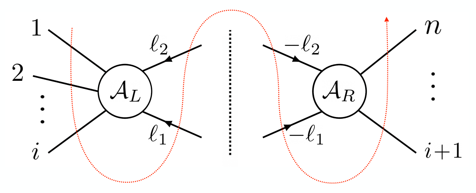
The generalization of Eq. (78) to loop amplitudes is straightforward. When the internal lines go on-shell, we need to add a factor per each fermion line. For example, let us consider the 2-cut of the loop amplitude of Fig. 14. We have
| (87) |
that leads to Eq. (16). Notice that the order of the states is important for fermions, that must follow the red dotted line as in Fig. 14.
B.2 SM Amplitudes
The on-shell amplitude approach is based on building higher-point amplitudes from already existing ones of lower . The basic “blocks” are the amplitudes, which are totally fixed by their helicities. For the SM gauge boson interactions, using the indices for the adjoint representation of the non-abelian groups, and indices for the fundamental representation, we have
| (88) | |||
| (89) |
For the abelian U(1)Y hypercharge we have similar expressions, with . We fix our normalization as , with and real . Let us comment that, in fact, only one of the amplitudes in Eqs. (88)–(89) is enough to fix the definition of the SM gauge coupling. For instance, once the gauge interaction to a fundamental fermion is defined, the gauge interaction to scalars can be determined by the consistency condition that amplitudes must factorize into products of amplitudes (this is the equivalent to gauge invariance in the Lagrangian approach – see for example [30]). Also, the second amplitudes in Eqs. (88)–(89) can be determined from the first using CPT invariance and unitarity.99 9 Unitarity , where and can be treated as a small perturbation around the identity, is needed to derive and therefore .
We also have Yukawa interactions, that for one family are given by (showing only the SU(2)L indices)
| (90) |
These amplitudes fix our definitions of the SM Yukawa couplings , that for one family can be taken to be real. The generalization to 3 families is straightforward. By CPT invariance and unitarity, we obtain
| (91) |
The relation between our gauge and Yukawa couplings, defined via amplitudes, and the usual definitions arising from Lagrangians is provided in Appendix C.
From the above amplitudes, we can build amplitudes. Here, we quote the ones that are needed for this work. These are amplitudes:
| (92) |
for ;
| (93) |
for ;
| (94) |
for . We also use and amplitudes, that are given by
| (95) |
| (96) |
All these amplitudes can be determined by just demanding proper transformation under the little group and factorization into amplitudes. Amplitudes for the opposite helicity, with particle interchanged with antiparticle, can be obtained by complex-conjugating the above ones.
Appendix C From the SM EFT Lagrangian to amplitudes
In this Appendix, we provide the relation between our on-shell amplitudes and operators used in the common Lagrangian approach for the SM EFT [8].
Let us start with the dimension-4 operators of the SM EFT. From our definition of the SM gauge couplings, given in Eqs. (88)–(89), we find that this corresponds to take the covariant derivative of a field transforming under the fundamental representation of the SM group as
| (97) |
where the generators are normalized as , and the hypercharge for the Higgs is . Notice that, as is usual in amplitude methods [1], our gauge couplings carry an extra , different from the more common definition of the SM gauge couplings. One can easily check that, indeed, the gauge vertices arising from Eq. (97) lead, by using Eq. (80) and Eq. (82), to Eqs. (88)–(89).
On the other hand, our Yukawa coupling defined in Eq. (90) corresponds to that arising from a Lagrangian term
| (98) |
where , and , being and Weyl spinors of , and similarly for the quarks.
At the dimension-6 level, we have
| (99) | |||||
| (100) | |||||
| (101) | |||||
| (102) | |||||
| (103) | |||||
| (104) | |||||
| (105) | |||||
| (106) | |||||
| (107) | |||||
| (108) | |||||
| (109) | |||||
| (110) | |||||
| (111) | |||||
| (112) |
The above formulas allow to relate the Wilson coefficients with the coefficients of the on-shell amplitudes that were used in this article.
Appendix D Dimension-5 operators and their corresponding on-shell amplitudes
Similarly as with the amplitudes at order (associated to dimension-6 operators), we can determine the extra contributions to amplitudes at order . These are given by
- •
n=3, h=-2:
(113) - •
n=4, h=-1:
(114) - •
n=5, h=0:
(115)
In the SM, only Eq. (114) is allowed by the gauge symmetry for , and it violates lepton number by two units.
One can show that Eq. (16) can also be applied to calculate the anomalous dimensions of the coefficients of these amplitudes. The proof goes as for the case: we know that Eq. (18) applies to any operator, so we can use it in the limit to get Eq. (16). We only have to be careful with potential extra contributions present in Eq. (18) that are not considered in Eq. (16). These are the ones involving amplitudes. In particular, they could be relevant in the renormalizations and . However, one can check that, in these one-loop renormalizations, all triangles and boxes lead to the same integrals as those discussed in Fig. 11, and so we can use the conclusions of Appendix A also here, to claim that the absence of IR divergencies imposes a cancellation of boxes and triangles in Eq. (16). Therefore Eq. (16) must coincide with Eq. (18) in the limit .
References
- [1] L. J. Dixon, “A brief introduction to modern amplitude methods,” arXiv:1310.5353 [hep-ph].
- [2] S. Caron-Huot and M. Wilhelm, JHEP 1612 (2016) 010 [arXiv:1607.06448 [hep-th]].
- [3] N. Arkani-Hamed, F. Cachazo and J. Kaplan, JHEP 1009 (2010) 016 [arXiv:0808.1446 [hep-th]].
- [4] N. Christensen and B. Field, Phys. Rev. D 98 (2018) no.1, 016014 [arXiv:1802.00448 [hep-ph]].
- [5] Y. Shadmi and Y. Weiss, JHEP 02 (2019), 165 [arXiv:1809.09644 [hep-ph]].
- [6] T. Ma, J. Shu and M. L. Xiao, [arXiv:1902.06752 [hep-ph]]; R. Aoude and C. S. Machado, JHEP 12 (2019), 058 [arXiv:1905.11433 [hep-ph]]; G. Durieux, T. Kitahara, Y. Shadmi and Y. Weiss, JHEP 01 (2020), 119 [arXiv:1909.10551 [hep-ph]]; G. Durieux and C. S. Machado, [arXiv:1912.08827 [hep-ph]];
- [7] J. Elias-Miro, J. R. Espinosa and A. Pomarol, Phys. Lett. B 747 (2015) 272 [arXiv:1412.7151 [hep-ph]].
- [8] B. Grzadkowski, M. Iskrzynski, M. Misiak and J. Rosiek, JHEP 10 (2010), 085 [arXiv:1008.4884 [hep-ph]].
- [9] T. Becher and M. Neubert, Phys. Rev. Lett. 102, 162001 (2009) doi:10.1103/PhysRevLett.102.162001 [arXiv:0901.0722 [hep-ph]].
- [10] Z. Bern, J. Parra-Martinez and E. Sawyer, Phys. Rev. Lett. 124 (2020) no.5, 051601 [arXiv:1910.05831 [hep-ph]].
- [11] Y. -t. Huang, D. A. McGady and C. Peng, Phys. Rev. D 87 (2013) no.8, 085028 [arXiv:1205.5606 [hep-th]].
- [12] D. Forde, Phys. Rev. D 75 (2007), 125019 doi:10.1103/PhysRevD.75.125019 [arXiv:0704.1835 [hep-ph]]. P. Mastrolia, Phys. Lett. B 678 (2009), 246-249 doi:10.1016/j.physletb.2009.06.033 [arXiv:0905.2909 [hep-ph]].
- [13] R. Britto, F. Cachazo, B. Feng and E. Witten, Phys. Rev. Lett. 94 (2005), 181602 doi:10.1103/PhysRevLett.94.181602 [arXiv:hep-th/0501052 [hep-th]].
- [14] C. Cheung and C. Shen, Phys. Rev. Lett. 115 (2015) no.7, 071601 [arXiv:1505.01844 [hep-ph]].
- [15] M. Jiang, J. Shu, M. L. Xiao and Y. H. Zheng, [arXiv:2001.04481 [hep-ph]].
- [16] N. Craig, M. Jiang, Y. Y. Li and D. Sutherland, [arXiv:2001.00017 [hep-ph]].
- [17] F. Boudjema, K. Hagiwara, C. Hamzaoui and K. Numata, Phys. Rev. D 43 (1991) 2223; B. Gripaios and D. Sutherland, Phys. Rev. D 89 (2014) no.7, 076004 [arXiv:1309.7822 [hep-ph]].
- [18] J. Elias-Miró, J. R. Espinosa, E. Masso and A. Pomarol, JHEP 1308 (2013) 033 [arXiv:1302.5661 [hep-ph]]; JHEP 11 (2013), 066 [arXiv:1308.1879 [hep-ph]].
- [19] E. E. Jenkins, A. V. Manohar and M. Trott, JHEP 1401 (2014) 035 [arXiv:1310.4838 [hep-ph]]. R. Alonso, E. E. Jenkins, A. V. Manohar and M. Trott, JHEP 1404 (2014) 159 [arXiv:1312.2014 [hep-ph]]; Errata: https://einstein.ucsd.edu/smeft/.
- [20] E. Braaten, C. S. Li and T. C. Yuan, Phys. Rev. Lett. 64 (1990), 1709.
- [21] G. Buchalla, A. Celis, C. Krause and J. N. Toelstede, [arXiv:1904.07840 [hep-ph]].
- [22] G. Panico, A. Pomarol and M. Riembau, JHEP 04 (2019), 090 [arXiv:1810.09413 [hep-ph]].
- [23] A. Pomarol, “Amplitudes meet BSM”, talk at Scalar 2019, Warsaw, September 2019. P. Baratella, “Aspects of Chiral Perturbation Theory from an on-shell perspective”, talk at COST Workshop: Probing BSM physics at different scales, Berlin, January 2020.
- [24] J. Elias Miro, J. Ingoldby and M. Riembau, [arXiv:2005.06983 [hep-ph]].
- [25] P. Baratella, C. Fernandez, B. von Harling and A. Pomarol, JHEP 03 (2021), 287 [arXiv:2010.13809 [hep-ph]].
- [26] R. Britto, J. Phys. A 44 (2011) 454006 [arXiv:1012.4493 [hep-th]].
- [27] H. Johansson, D. A. Kosower and K. J. Larsen, PoS LL 2012 (2012) 066 [arXiv:1212.2132 [hep-th]].
- [28] H. K. Dreiner, H. E. Haber and S. P. Martin, Phys. Rept. 494 (2010), 1-196 [arXiv:0812.1594 [hep-ph]].
- [29] M. L. Mangano and S. J. Parke, Phys. Rept. 200 (1991), 301-367 [arXiv:hep-th/0509223 [hep-th]].
- [30] N. Arkani-Hamed, T. Huang and Y. Huang, [arXiv:1709.04891 [hep-th]].