Reinforced Coloring for End-to-End
Instance Segmentation
Abstract
Instance segmentation is one of the actively studied research topics in computer vision in which many objects of interest should be separated individually. While many feed-forward networks produce high-quality segmentation on different types of images, their results often suffer from topological errors (merging or splitting) for segmentation of many objects, requiring post-processing. Existing iterative methods, on the other hand, extract a single object at a time using discriminative knowledge-based properties (shapes, boundaries, etc.) without relying on post-processing, but they do not scale well. To exploit the advantages of conventional single-object-per-step segmentation methods without impairing the scalability, we propose a novel iterative deep reinforcement learning agent that learns how to differentiate multiple objects in parallel. Our reward function for the trainable agent is designed to favor grouping pixels belonging to the same object using a graph coloring algorithm. We demonstrate that the proposed method can efficiently perform instance segmentation of many objects without heavy post-processing.
Keywords:
Image segmentation, deep reinforcement learning1 Introduction
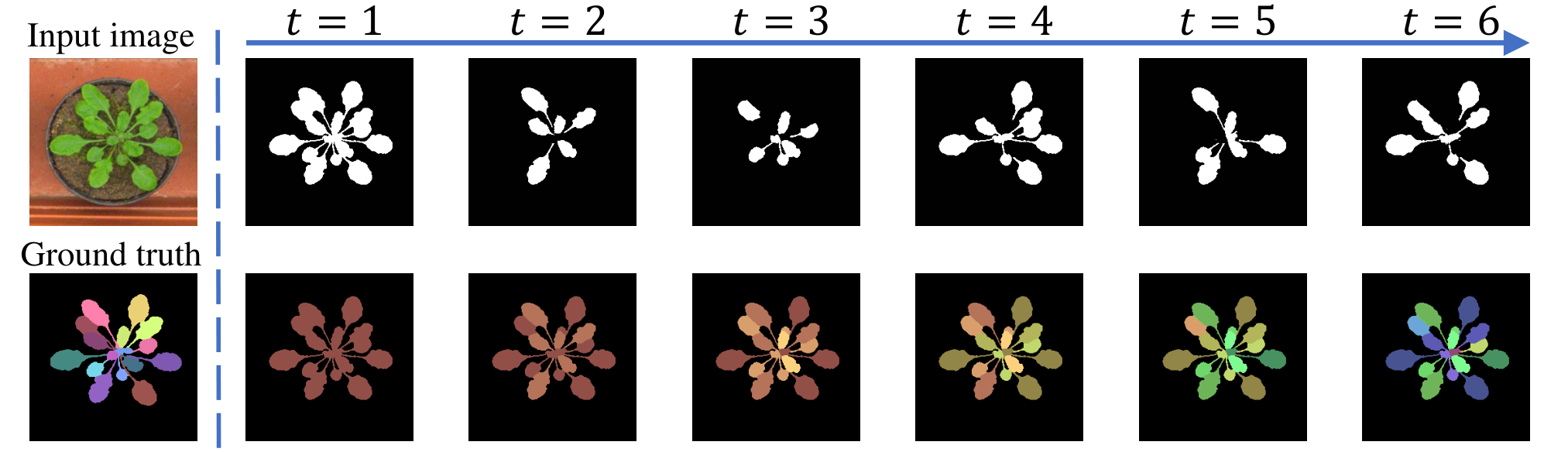
Recent advances in deep reinforcement learning (DRL) has archived human-level performance on complicated tasks that previously required human control and decision making [21, 17, 30]. Given that the training reinforcement learning agent learns tasks in a human-like way (from experience via trial and error), the early success of DRL mainly focused on mimicking human tasks, such as playing games. More recently, there have also been successful attempts to apply DRL in conventional computer vision tasks, such as image processing [8, 16].
Instance segmentation is a challenging computer vision problem that assigns instance labels to pixels to separate objects, which is crucial for understanding a complex scene. Many existing instance segmentation methods arebased on complicated graphical models with deep neural networks (e.g., convolutional neural network [CNN] or recurrent neural network [RNN])) [34, 33, 26]. However, instance segmentation also involves decision tasks (i.e., how to assign labels to pixels), which is more complicated than conventional (semantic) object segmentation. Recent work by Araslanov et al. aimed to addressed this issue by employing reinforcement learning for the sequential object detection and segmentation task [2].
While sequential object segmentation methods like those of Araslanov et al. and Ren et al. [26] have shown promising results on image with a small number of objects, their sequential methods, which segments one object at a time, are not efficient when the number of objects is large. To address this problem, we propose a novel end-to-end instance segmentation method using reinforcement learning. Unlike the method where a single agent handles an object as seen in Araslanov et al., our coloring agent consists of multiple pixel-level agents (as in Furuta et al. [8]) working concurrently to differentiate multiple objects in a sequential, end-to-end fashion (fig. 1). To enable multiple instances to be labeled concurrently, we formulate and solve an iterative graph binary coloring problem. Using the asynchronous advantage actor-critic (A3C) algorithm, our agents are trained to choose the -th bit value in binary representation of the label at the step of the coloring process. Pixel-label agents try to take actions (0 or 1) that are either matching or different at one point throughout the coloring process, depending on whether the instances are same or different.
To the best of our knowledge, this is the first end-to-end instance segmentation that uses reinforcement learning. We demonstrate the performance and scalability of the proposed method on several open source datasets, such as KITTI [9], CREMI [6], and CVPPP [19] and compare our results with the other iterative methods. We demonstrate that our method can efficiently handle images with many objects of various shapes while still maintaining a competitive segmentation quality.
2 Related Work
In this section, we briefly overview the recent advances in image segmentation methods, which are closely related to the instance segmentation problem.
Knowledge-based segmentation approaches: Conventionally, prior knowledge can be used to incorporate to a representation (e.g., a computational graph where pixels become nodes and the quantitative relationship between them form edges). Solving the min-cut and max-flow in this relationship can partition an image into discriminative regions (or segmentation) [3]. The key idea in these approaches is to construct a proper distance metric between pixels so that they can be grouped into segments where the total number of partitions can be either deterministic or not [1]. However, hand-crafted prior knowledge from those clusters is not always aligned to the goal of segmentation and left a room for improvement.
Supervised learning approaches: The invention of Fully Convolutional Neural Network (FCN) [18] and its variations, such as U-net [28] with different backbones [12, 13] and different types of skip-connection [25, 14], have achieved a big success in segmentation tasks. Moreover, one can focus on the loss function design that makes it possible for a cluster to collapse by itself into one region and push other clusters far away [7]. Another direction for solving the instance segmentation task is to produce segmentation in a sequential prediction manner. Ren et al. [26] utilize a recurrent neural network to perform step-by-step performing attention then segmentation the mask of a single object. This approach returns a good segmentation map for the image and also accurately returns the number of object, but does not scale well for many objects. The advantage of supervised learning approaches is that the level of hierarchical order of segmentation can be obtained directly from the data without complicated hand-crafted rules, but most methods are still sequential.
Reinforcement learning approaches: Since Mnih et al. [21] introduced their seminal work, an increasing number of complex tasks that are challenged by machine intelligence due to its complex sequences of decision making processes have been solved by reinforcement learning [30, 15, 17]. It is natural for one to seek to make use of the recent advancements in reinforcement learning and apply them to solve the problem in the computer vision domain. For example, Furuta et al. presented an efficient way to train an asynchronous actor critic agent (A3C), which is called PixelRL [8], that uses the decision making per pixel for the denoising problem. To investigate how those sequential steps can form the segmentation solution pipeline, people have constructed the segmentation procedure as a Markov Decision Process (MDP) and attempted to solve it by leveraging several state-of-the-art algorithms in reinforcement learning. Araslanov et al. [2] formulated the instance-aware segmentation problem into a sequential object detection-segmentation action decision making process. Gwangmo et al. [31] made an agent that uses the random walk segmentation algorithm [11] with human interaction input to sequentially extract the region of interest. However, it is still lacking a method that can segment multiple objects at a time in a sequential manner.
3 Graph Coloring Approach
3.1 Problem Formulation
In this work, we formulate the instance segmentation problem into a multi-step graph coloring problem, similar to D. Gómez et al. [10]. Given that image I consists of the set of pixels . A segmentation of I partitions into , where each belongs to exactly one for and . By constructing the set of edges and graph from , we can formulate the instance segmentation problem into a graph coloring problem. For each image I, we want to find a color (label) mapping that assigns a color to every pixel, , that satisfies the following constraints. Given a graph and a ground truth partitioning of : if s.t and and ; if s.t and and . Then, the image segmentation problem is finding a proper function that maps a set of graphs to the set of color mapping that satisfies the above constrains.
Since the task of finding an optimal is an NP-Hard problem [5], so we find the approximation of using an iterative binary coloring process. We begin by letting be the color mapping of at time step ; and defining coloring action , where maps to , and is the size of . Each of is mapped to or though . denotes the mapped value of , and the color of at time step is computed as follows (we illustrate this function in Figure 2):
| (1) |
Here returns the color mapping of a single vertex in . If T is the maximum number of coloring steps, then we have a -step approximation function of , which maps to . It can be seen that is assigned to the -th digit in the binary representation of color of .
3.2 A3C and PixelRL
For the coloring problem, we can naturally think of a multi-agent system where each agent is in charge of taking action that changes for a single vertex of . Asynchronous actor critic (A3C) is one of the policy gradient algorithms that has demonstrated high performance for discrete action space decision-making problems [20]. In this work, we employed the method introduced by Furuta et al. [8] which uses an efficient technique for a multi-agent system (PixelRL) which works well with A3C.
An image I has a set of pixels in PixelRL problem setting. Each has a corresponding state at time step . A pixel-level agent with policy is assigned to each pixel . State and reward are obtained from the environment by taking action , . In our work, has only two values, and , which represent the binary digit value of label color. The agents try to maximize the mean of their total expected reward:
| (2) |
| (3) |
where is the mean rewards . At each time step , with state , PixelRL agent computes the value function and policy function . estimates the expected reward an agent can get from the state , which implies how good the state is. Loss functions of and of for a single agent at pixel are computed as follows:
| (4) |
| (5) |
where is the advantage function, which shows how good the action at step is compared to the expected return. At each time step , gradients for value loss and policy loss are computed and used to update the parameters of and . In PixelRL, a convolutional neural network is used to compute and ; and have the same dimensions as the input image . For more information, see Furuta et al. [8].
3.3 Coloring Agent

Our coloring agent processes the state at time step to produce a binary map of actions, and each action makes a change for a single pixel label.
The action map is also a binary mask of multiple-object segmentation.
We formulate the Markov Decision Process for the instance segmentation problem with the tuple of state, action, and reward.
Figure 3 shows an overview of the agent architecture.
This section will explain these three terms in detail.
State:
Function takes the input, which is a set of vertices (the image I), and its color map .
Given image I of size , the representation of input and for here are the image I and its binary encoded -channels color map.
Thus, the state of an agent is an image of size , where T is the number of coloring steps.
Here, is the channels of image I and is the number of binary digits of color map.
Actions:
Action map that resulted from is a binary image of size as defined in Section 3.1. The action map at the time step can be seen as a segmentation map of several objects at that time step.
Rewards:
For each pixel, to get the reward map , we need to construct the set of edges between pixels from the ground truth label and .
The goal of the reward function for each action is to give reasonable feedback for the actions that cause pixels to have different colors (splitting actions) and the actions that keep pixels having the same colors (merging actions).
We divide the reward function into three major components, one that encourages the splitting actions, another that encourages merging actions, and the third one that classifies between foreground and background labels.
Figure 4 illustrates the edges construction phase for the computation of reward function.
To make the reward function more instance-focused, the edges are constructed only between foreground pixels while the separation between foreground and background is done specially at first step with a designated reward component.
We denote be the ground truth label of pixel , and when of the background only.
is the ground truth segment that contains (ie. ).
Reward for predicting background-foreground:
We design a reward function just to segmenting between background region and foreground region.
By doing this, the background pixels do not need to compare with each other (especially when the image has complex background structures like in electron microscope (EM) images).
The reward function for separating foreground and background is defined as follows:
| (6) |
Here, we set and to be the percentage of the foreground and background areas to the entire area, respectively.
In the first step, we made the problem to be only differentiating between foreground and background.
After that, our agent separates objects while maintaining the background prediction.
Thus, the foreground components ( and ) are given only in the first step (at ).
Reward for spliting actions:
By constructing edges between pixels of different ground truth (GT) segments, we wish to compare their color and give feedback to the actions that return the color mapping.
Given the positive integer , the edge list constructed using is denoted as .
A directed edge originating from to is defined as a tuple ().
Then if and and and s.t where is the Manhattan distance between and .
can be considered as the radius of segments, so we call a splitting radius.
Figure 4a illustrates how edges originating from are constructed using a given splitting radius .
We then define the set
and for a pixel at time step as follows:
| (7) |
| (8) |
As outlined above, and can be represented as the set of neighborhoods of that are correctly split and incorrectly merged.
For a pixel with radius , at time step , the splitting reward is computed as follows:
| (9) |
| (10) |
| (11) |
| (a) Edge construction for splitting | (b) Edge construction for merging |
Reward for merging actions: We construct edges between pixels in the same ground truth segment for the merging reward function. The reward function guides the pixel-level agents from the same ground truth segment to take the same actions. For an object, it is more important for the pixels of the inner region to have the same color with each other than for a pixels of the outer region to have the same color with other pixels inside the object. We give a higher priority for matching color between pixels in the inner region. Given a shrinking factor (), the inner region of a ground truth segment containing is generated by shrinking to such that or . The directed edge list is constructed as follows (illustration of the graph construction is in Figure. 4): if and . We then define the set and for a pixel at time step as follow:
| (12) |
| (13) |
and are the set of neighborhoods of that are wrongly split from and correctly merged with . For a pixel with shrinking factor at time step (), the merging reward is computed as follows:
| (14) |
| (15) |
| (16) |
Reward for pixel at time step :
Our reward function for a vertex is described as follow:
When :
| (17) |
and when :
| (18) |
where and are weights for merging and splitting, respectively. and are the sets of (s) and (s) for different values of and , respectively. The higher the value for compared to , the higher the chance that actions that keep the merged area intact will be chosen, and vice versa.
4 Experiments and Results
In this work, we used Attention U-Net architecture (AttU) [22] for the core network of our agent. Due to the difference between input image space and label color space, we let input image I and the binary color map go though two different paths before merging them by concatenation as input for AttU, as shown in the overview structure (Fig. 3). For pre-processing modules, we use astrous spatial pooling layers. We set the discount factor with the default value of and shrinking factor in all the experiments.

 |
|
| (a) | (b) |

4.1 Ablation Study
Splitting radius setting:
Separating objects within close proximity is more important and challenging.
By exploiting different levels of splitting radius (s), the agent can learn to do segmentation better. Here, we analyze the behavior of our agent with two levels of splitting radii and . The environment setting becomes simpler as we let the agent to only learn to segment a single training image (no augmentation and also).
We observed that and gave the best result among the trials (Fig. 5).
While a small radii setting gives the agent enough information to differentiate close and small objects, there is no feedback for the agent to separate large and far apart instances ().
A large radii setting, on the other hand, gives long-distance information but also makes the task harder as the pixels have to process more ().
Too small () or too big radius () components can also guide the agent poorly as too small radii often contribute almost no useful information and too large radii make the task much harder.
Weights for splitting and merging rewards: We analyzed how the reward functions affect the agent by testing different sets of weights for splitting and merging rewards.
We used 103 training images and 25 validation images of CVPPP, and fixed the sum of and to a constant of 2 in this experiment. The results using different weight settings are shown in Table 1 and Figure 7. We see that the low merge-split weight ratio does affect the segmentation quality of our reinforced coloring agent (RC) as much high merge-split weight ratio.
| Model | SBD | DiC | ||||
|---|---|---|---|---|---|---|
| 0.00 | 2.00 | 21.2 | 15.6 | |||
| 0.25 | 1.75 | 21.2 | 9.44 | |||
| 0.50 | 1.50 | 70.7 | 2.72 | |||
| RC | 1.00 | 1.00 | 12 | 28 | 85.2 | 1.40 |
| 1.50 | 0.50 | 87.3 | 1.34 | |||
| 1.7 | 0.25 | 81.4 | 1.44 | |||
| 2.00 | 0.00 | 5.60 | 92.8 |
We observed that during the training and exploration for better decision making, our agent reaches the easier stage first (maximization of merging reward) then gradually finds actions that differentiate objects (maximization of splitting reward) (Fig. 6a). During the latter stages, maximizing splitting rewards may come with the cost of merging reward at some point (Fig. 6b). Thus, it is necessary that for the trade-off of splitting and merging rewards. Based on this result, for all the experiments discussed in the following sections, we choose and for a little higher incentive to the agent for exploring splitting actions. While is always set to to relax the learning difficulty of instance border areas, we use different splitting radius for different datasets.
4.2 CVPPP Dataset
| Model | SBD | DiC |
|---|---|---|
| RIS [27] | 66.6 | 1.1 |
| MSU [29] | 66.7 | 2.3 |
| Nottingham [29] | 68.3 | 3.8 |
| IPK [24] | 74.4 | 2.6 |
| DLoss [7] | 84.2 | 1.0 |
| E2E [26] | 84.9 | 0.8 |
| AC-Dice [2] | 79.1 | 1.12 |
| Ours (RC) | 80.0 | 1.36 |
The Computer Vision Problems in Plants Phenotyping (CVPPP) dataset is one of the popular datasets used for assessing the performance of instance segmentation algorithms. We used the A1 dataset, which consists of 128 training images and 33 testing images. We resized the images down to pixels (the original size was pixels) and used two levels of splitting radius and as discussed in Section 4.1.

We allow our agent to use the same label color for objects that are far apart from each other. For the sake of the evaluation, for all the data sets, before the evaluation of segmentation accuracy, the predicted label map is further post-processed with resizing (upscaling to the original size), removing small segments, and re-indexing labels. The evaluation is done on the original size of the data. The quality of the segmentation is measured in the Symmetric Best Dice (SBD) and the absolute Difference in Counting (DiC) measurements. The checkpoint used for the evaluation is selected from the one that has the best DiC score. Comparing our results with Ren et al. (E2E) and Araslanov et al. (AC-Dice), while our DiC score is slightly lag behind, our agent produces segmentation quality on par with their methods (see Table 2). Figure 8 shows that our agent can segment the leaves also handle occlusions well.
4.3 KITTI Dataset
| Model | MWCov | MUCov | AvgFP | AvgFN |
|---|---|---|---|---|
| DepthOrder [34] | 70.9 | 52.2 | 0.597 | 0.736 |
| DenseCRF [33] | 74.1 | 55.2 | 0.417 | 0.833 |
| AngleFCN+D [32] | 79.7 | 75.8 | 0.201 | 0.159 |
| E2E [26] | 80.0 | 66.9 | 0.764 | 0.201 |
| AC-BL-Trunc [2] | 72.2 | 50.7 | 0.393 | 0.432 |
| AC-IoU [2] | 75.6 | 57.3 | 0.338 | 0.309 |
| Ours (RC) | 77.0 | 68.5 | 0.249 | 0.128 |
We also assess the performance of our method on the KITTI car segmentation dataset. We use the same 3712 images for training, 144 images for validation and 120 images for testing as in [2, 26]. In KITTI dataset, the training labels generated from [23] are in a coarse resolution but the testing and validation images are in a high resolution, which makes the problem challenging [23, 4]. We downsampled the training images to (originally pixels). Since vehicles in KITTIS are often distributed sparsely in the images and their number is also small, we set our agent to do 4-step coloring. In this data, we use two levels of the radius ( and ). The post-processing setting for evaluation is the same as the setting we used with CVPPP.
The metrics used for evaluation of this data are the mean weighted coverage (MWCow), the mean unweighted coverage loss (MWCow), the average false positive rate (AvgFP), and the average false negative rate (AvgFN). MUCow measures the instance-wise IoU for each GT instance averaged over the image, while MWCow is the average of IoUs of predicted labels matched with GT instances weighted by the size of GT instances [26]. AvgFP is the fraction of predicted label segments that do not have matched GT segments. AvgFN is the fraction of GT label segments that do not have a matched label prediction. Our result is shown in Table 3, which illustrates that our AvgAP and AvgFN scores are better than Ren et al. and Araslanov et al.’s single-object-per-step approaches. Previous comparison with result from Figure 8 demonstrate that our method can learn and generalize well from the incomplete annotation.
4.4 CREMI Dataset

| Model | Data type | avg. time(ms) | VOI-split | VOI-merge | ARand |
|---|---|---|---|---|---|
| E2E [26] | Type I | 514.83 | 0.772 | 0.544 | 0.276 |
| Ours | 171.76 | 0.412 | 0.113 | 0.07 | |
| E2E [26] | Type II | 910.46 | 1.178 | 3.082 | 0.660 |
| Ours | 186.97 | 0.379 | 0.230 | 0.095 |
CREMI is an electron microscope image dataset in which many cell objects are densely packed. We chose this dataset to demonstrate both the segmentation quality and the scalability of our method. We used a padded version of CREMI dataset A, which has 125 sections of images of pixels. We prepared two versions of the dataset from the original one: type I and type II. Dataset type I has patches of size pixels and each patch has 24 cells on average (maximum is 40). Dataset type II has patches of size , and each patch has on average 65 cells (80 at most). For each type, we randomly extract 103 patches from the first 100 sections for the training set and 25 patches from the last 25 sections for the test set. Training images were downsampled to .
Quality metrics used in this experiment are a Variation of Information (VOI-split, VOI-merge), adapted RAND error (ARAND), and mean inference time per patches (.avg time). Figure 9 and Table 4 show that our agent can capture better shape and size of cells. While E2E can find and segment densely packed cells (although not perfect) in type I images, the method easily loses its tracking of cells (large regions are classified as background) in type II images. CREMI images contain many cells of complex structures and varying sizes as well as noise and occlusions, which makes the problem more challenging for the attention-then-segmentation approach like E2E. Our method, on the other hand, can effectively handle densely packed many objects by separating multiple objects in parallel via iterative binary segmentation (i.e., graph coloring). The average inference time (Avg.time) is also measured (post-processing time is included). While the inference time of E2E linearly increases with the number of objects, our average inference time stayed constant, which shows the superior scalability of our method.
5 Conclusion
In this paper, we introduced a novel per-pixel label assignment method for end-to-end instance segmentation based on a graph coloring approach. We proposed a reward function that gives meaningful feedback for each pixel to decide its label index iteratively. Based on the evaluation of three datasets (KITTI, CVPPP, and CREMI), we demonstrated that the proposed method is effective for instance segmentation of many objects. In the future, we plan to conduct rigorous performance the evaluation on large-scale multiple-object segmentation.
References
- [1] Achanta, R., Shaji, A., Smith, K., Lucchi, A., Fua, P., Süsstrunk, S.: Slic superpixels. Tech. rep. (2010)
- [2] Araslanov, N., Rothkopf, C.A., Roth, S.: Actor-critic instance segmentation. In: Proceedings of the IEEE Conference on Computer Vision and Pattern Recognition. pp. 8237–8246 (2019)
- [3] Boykov, Y., Funka-Lea, G.: Graph cuts and efficient nd image segmentation. International journal of computer vision 70(2), 109–131 (2006)
- [4] Chen, X., Kundu, K., Zhang, Z., Ma, H., Fidler, S., Urtasun, R.: Monocular 3d object detection for autonomous driving. In: Proceedings of the IEEE Conference on Computer Vision and Pattern Recognition. pp. 2147–2156 (2016)
- [5] Cormen, T.H., Leiserson, C.E., Rivest, R.L., Stein, C.: Introduction to algorithms (2009)
- [6] CREMI: Miccai challenge on circuit reconstruction from electron microscopy images (2016), https://cremi.org/
- [7] De Brabandere, B., Neven, D., Van Gool, L.: Semantic instance segmentation with a discriminative loss function. arXiv preprint arXiv:1708.02551 (2017)
- [8] Furuta, R., Inoue, N., Yamasaki, T.: Fully convolutional network with multi-step reinforcement learning for image processing. In: Proceedings of the AAAI Conference on Artificial Intelligence. vol. 33, pp. 3598–3605 (2019)
- [9] Geiger, A., Lenz, P., Urtasun, R.: Are we ready for autonomous driving? the kitti vision benchmark suite. In: 2012 IEEE Conference on Computer Vision and Pattern Recognition. pp. 3354–3361. IEEE (2012)
- [10] Gómez, D., Montero, J., Yáñez, J., Poidomani, C.: A graph coloring approach for image segmentation. Omega 35(2), 173–183 (2007)
- [11] Grady, L.: Random walks for image segmentation. IEEE Transactions on Pattern Analysis & Machine Intelligence (11), 1768–1783 (2006)
- [12] He, K., Zhang, X., Ren, S., Sun, J.: Deep residual learning for image recognition. In: Proceedings of the IEEE conference on computer vision and pattern recognition. pp. 770–778 (2016)
- [13] Huang, G., Liu, Z., Van Der Maaten, L., Weinberger, K.Q.: Densely connected convolutional networks. In: Proceedings of the IEEE conference on computer vision and pattern recognition. pp. 4700–4708 (2017)
- [14] Jégou, S., Drozdzal, M., Vazquez, D., Romero, A., Bengio, Y.: The one hundred layers tiramisu: Fully convolutional densenets for semantic segmentation. In: Proceedings of the IEEE Conference on Computer Vision and Pattern Recognition Workshops. pp. 11–19 (2017)
- [15] Kempka, M., Wydmuch, M., Runc, G., Toczek, J., Jaśkowski, W.: Vizdoom: A doom-based ai research platform for visual reinforcement learning. In: 2016 IEEE Conference on Computational Intelligence and Games (CIG). pp. 1–8. IEEE (2016)
- [16] Li, D., Wu, H., Zhang, J., Huang, K.: A2-rl: Aesthetics aware reinforcement learning for image cropping. In: Proceedings of the IEEE Conference on Computer Vision and Pattern Recognition. pp. 8193–8201 (2018)
- [17] Lillicrap, T.P., Hunt, J.J., Pritzel, A., Heess, N., Erez, T., Tassa, Y., Silver, D., Wierstra, D.: Continuous control with deep reinforcement learning. arXiv preprint arXiv:1509.02971 (2015)
- [18] Long, J., Shelhamer, E., Darrell, T.: Fully convolutional networks for semantic segmentation. In: Proceedings of the IEEE conference on computer vision and pattern recognition. pp. 3431–3440 (2015)
- [19] Minervini, M., Fischbach, A., Scharr, H., Tsaftaris, S.A.: Finely-grained annotated datasets for image-based plant phenotyping. Pattern recognition letters 81, 80–89 (2016)
- [20] Mnih, V., Badia, A.P., Mirza, M., Graves, A., Lillicrap, T., Harley, T., Silver, D., Kavukcuoglu, K.: Asynchronous methods for deep reinforcement learning. In: International conference on machine learning. pp. 1928–1937 (2016)
- [21] Mnih, V., Kavukcuoglu, K., Silver, D., Rusu, A.A., Veness, J., Bellemare, M.G., Graves, A., Riedmiller, M., Fidjeland, A.K., Ostrovski, G., et al.: Human-level control through deep reinforcement learning. Nature 518(7540), 529–533 (2015)
- [22] Oktay, O., Schlemper, J., Folgoc, L.L., Lee, M., Heinrich, M., Misawa, K., Mori, K., McDonagh, S., Hammerla, N.Y., Kainz, B., et al.: Attention u-net: Learning where to look for the pancreas. arXiv preprint arXiv:1804.03999 (2018)
- [23] Papandreou, G., Chen, L.C., Murphy, K.P., Yuille, A.L.: Weakly-and semi-supervised learning of a deep convolutional network for semantic image segmentation. In: Proceedings of the IEEE international conference on computer vision. pp. 1742–1750 (2015)
- [24] Pape, J.M., Klukas, C.: 3-d histogram-based segmentation and leaf detection for rosette plants. In: European Conference on Computer Vision. pp. 61–74. Springer (2014)
- [25] Quan, T.M., Hildebrand, D.G., Jeong, W.K.: Fusionnet: A deep fully residual convolutional neural network for image segmentation in connectomics. arXiv preprint arXiv:1612.05360 (2016)
- [26] Ren, M., Zemel, R.S.: End-to-end instance segmentation with recurrent attention. In: CVPR (2017)
- [27] Romera-Paredes, B., Torr, P.H.S.: Recurrent instance segmentation. In: European conference on computer vision. pp. 312–329. Springer (2016)
- [28] Ronneberger, O., Fischer, P., Brox, T.: U-net: Convolutional networks for biomedical image segmentation. In: International Conference on Medical image computing and computer-assisted intervention. pp. 234–241. Springer (2015)
- [29] Scharr, H., Minervini, M., French, A.P., Klukas, C., Kramer, D.M., Liu, X., Luengo, I., Pape, J.M., Polder, G., Vukadinovic, D., et al.: Leaf segmentation in plant phenotyping: a collation study. Machine vision and applications 27(4), 585–606 (2016)
- [30] Silver, D., Huang, A., Maddison, C.J., Guez, A., Sifre, L., Van Den Driessche, G., Schrittwieser, J., Antonoglou, I., Panneershelvam, V., Lanctot, M., et al.: Mastering the game of go with deep neural networks and tree search. nature 529(7587), 484 (2016)
- [31] Song, G., Myeong, H., Mu Lee, K.: Seednet: Automatic seed generation with deep reinforcement learning for robust interactive segmentation. In: Proceedings of the IEEE Conference on Computer Vision and Pattern Recognition. pp. 1760–1768 (2018)
- [32] Uhrig, J., Cordts, M., Franke, U., Brox, T.: Pixel-level encoding and depth layering for instance-level semantic labeling. In: German Conference on Pattern Recognition. pp. 14–25. Springer (2016)
- [33] Zhang, Z., Fidler, S., Urtasun, R.: Instance-level segmentation for autonomous driving with deep densely connected MRFs. In: Proceedings of the IEEE Conference on Computer Vision and Pattern Recognition. pp. 669–677 (2016)
- [34] Zhang, Z., Schwing, A.G., Fidler, S., Urtasun, R.: Monocular object instance segmentation and depth ordering with CNNs. In: Proceedings of the IEEE International Conference on Computer Vision. pp. 2614–2622 (2015)