Abstract
Heavy-heavy-light-light (HHLL) correlators of pairwise identical scalars in CFTs with a large central charge in any number of dimensions admit a double scaling limit where the ratio of the heavy conformal dimension to the central charge becomes large as the separation between the light operators becomes null. In this limit the stress tensor sector of a generic HHLL correlator receives contributions from the multi stress tensor operators with any number of stress tensors, as long as their twist is not increased by index contractions. We show how one can compute this leading twist stress tensor sector when the conformal dimension of the light operators is large and the stress tensor sector approximates the thermal CFT correlator. In this regime the value of the correlator is related to the length of the spacelike geodesic which approaches the boundary of the dual asymptotically AdS spacetime at the points of light operator insertions. We provide a detailed description of the infinite volume limit. In two spacetime dimensions the HHLL Virasoro vacuum block is reproduced, while in four spacetime dimensions the result is written in terms of elliptic integrals.
1. Introduction: In -dimensional CFTs with a large central charge there are multi-stress tensor operators composed out of stress-tensors and derivatives. The contribution of such composite operators to a four-point function forms the stress-tensor sector of this correlator. The case where the correlator includes two pairwise identical operators with conformal dimension of order unity and two identical heavy operators with conformal dimension (with the ratio fixed) has recently been studied in various ways Kulaxizi et al. 2019a; Fitzpatrick and Huang 2019; Karlsson et al. 2019; Li et al. 2019; Kulaxizi et al. 2019b; Fitzpatrick et al. 2019; Karlsson et al. 2020a; Li 2019; Karlsson 2019; Karlsson et al. 2020b; Li and Zhang 2020.
Such heavy-heavy-light-light (HHLL) correlators can be used to determine the OPE coefficients of the two light operators with the multi-stress tensors; with this data one can compute the stress tensor sector of any correlator. In CFTs with holographic duals Maldacena 1999; Witten 1998a; Gubser et al. 1998 we expect generic heavy states created by to thermalize; thermal holographic CFTs are described by asymptotically AdS black holes Witten 1998b. (For recent work on thermalization in CFTs see e.g. Lashkari et al. 2018a; Lashkari et al. 2018b; Dymarsky and Pavlenko 2019.) Hence, the HHLL correlators provide a window into thermal correlators in CFTs.
It will be convenient to place the CFT on a lorentzian cylinder whose base is a ()-dimensional sphere of radius . Consider a kinematical setup where the heavy operators create a heavy state in the infinite past (and annihilate it in the future) while the light operators approach each other’s lightcone from the spatial direction. In the language of conformal cross-ratios , this corresponds to taking () to zero, while keeping fixed. In this case the main contribution to the term in the stress tensor sector comes from the multi stress operators with stress tensors with minimal twist . An interesting double-scaling limit involves taking large, keeping fixed 11 1 As explained in Section 2, is the separation between the insertions of the light operators in the rescaled lightlike direction.. In this limit all minimal twist multi stress tensor operators contribute.
In Fitzpatrick and Huang 2019 it was argued, in a holographic setting, that the OPE coefficients of such operators with two light scalars are universal, i.e. do not depend on the gravitational lagrangian in the bulk. A procedure for computing these OPE coefficients using lightcone conformal bootstrap Fitzpatrick et al. 2013; Komargodski and Zhiboedov 2013 was proposed in Karlsson et al. 2020a. At each twist there are infinitely many multi stress tensors labeled by spin, but one can perform the summation and obtain a simple expression Kulaxizi et al. 2019b. As argued in Karlsson et al. 2020a, the leading twist part of the stress tensor sector exponentiates:
| (1) |
where is a universal function which can be computed order by order in Karlsson et al. 2020a and has a finite limit as , which we denote by . Hence, the situation is very similar to that in two spacetime dimensions, where the HHLL Virasoro vacuum block also has the form (1). The HHLL Virasoro block was computed exactly in a variety of ways (see e.g. Fitzpatrick et al. 2014; Fitzpatrick et al. 2015; Hijano et al. 2015a; Hijano et al. 2015b; Fitzpatrick et al. 2016; Cotler and Jensen 2019; Collier et al. 2018).
The situation in is much more intricate and the function is not known. In this paper we use holography to compute . Note that in the limit the multi-trace operators which include one or more insertion of decouple and the stress tensor sector approximates the full thermal correlator, at least for holographic theories. The value of equals minus the (regularized) length of the spacelike geodesic which propagates in the -dimensional AdS-Schwarzschild background and approaches the positions of the light operator insertions at the boundary. This has recently been used to partially compute the multi stress tensor OPE coefficients Fitzpatrick and Huang 2019; Kulaxizi et al. 2019b (see also Maxfield 2017). We pay particular attention to the large volume limit, where and . In this case the function simplifies and we provide direct comparison (and exact matching) for the first few terms in the expansion.
The rest of the paper is organized as follows. In the next Section we provide a brief review and set up notation along the way. In Section 3 we compute the effective metric where the geodesic, whose length computes the near lightcone correlator, propagates. We also write down expressions which allow the computation of . In Section 4 we consider the large volume limit and reproduce the Virasoro vacuum block in . We also compute in the four-dimensional case and match the first few terms in the expansion in with the known results. We discuss the results in Section 5. Appendix A contains some details related to the case, while Appendix B describes the case.
2. Review: We will consider the stress-tensor sector of the correlator, where the heavy operators are inserted at , and the relative coordinates of the light operators differ by in the time direction and by on the ()-sphere. The contribution of the multi stress-tensors (denoted by the subscript ”MST”) can be written as
| (2) |
The conformal dimension of the heavy operators, , is proportional to the central charge with
| (3) |
fixed. The cross-ratios and are related to the relative spacetime positions of the light operators as (see e.g. Kulaxizi et al. 2019a)
| (4) |
where
| (5) |
In the equations above, and in most of what follows we set . To retain the contributions of all leading twist multi stress tensors we take the double-scaling limit with
| (6) |
fixed. The double scaling limit of the stress-tensor sector of the HHLL correlator, which we denote by , exponentiates,
| (7) |
In (7) receives contributions from the minimal twist multi-stress tensor operators with stress tensors. In the function is -independent,
| (8) |
In higher dimensions it is possible to compute using conformal bootstrap, order by order in . The terms is just the stress tensor contribution, where . The term is a result of the summation of all twist- double stress tensors with varying spin (one can find the explicit expression for in Kulaxizi et al. 2019b). It will be useful to consider the limit of the term,
| (9) |
The next, term in the expansion, was computed using bootstrap in Karlsson et al. 2020a. To take the large volume limit one needs to set the hypergeometric functions in to unity. (This corresponds to keeping only multi stress tensors without derivatives). The result is
| (10) |
where we used (4) to write the result in terms of . The first term in the right hand side of (10) corresponds to the vacuum two-point function.
3. Effective metric and spacelike geodesics: We would like to analyze spacelike geodesics in ()-dimensional AdS-Schwarzschild spacetime:
| (11) |
where
| (12) |
As discussed above, we are interested in the limit . We will consider spacelike geodesics which approach the AdS boundary at points separated in the lightlike direction by with fixed 22 2 In the following we mostly consider , but the limit can also be recovered.. The geodesics can be taken to live in the part of the spacetime. It is natural to write the metric (11) in coordinates , and . In the limit the metric of the three-dimensional spacetime where the geodesics propagate becomes
| (13) |
The two Killing vectors give rise to two conserved quantities,
| (14) |
The geodesic equation becomes
| (15) |
Eq. (15) describes the one-dimensional motion of a particle in an effective potential which can be inferred from (15). An important quantity is the largest (real) solution of the equation
| (16) |
It specifies the turning point of the particle. Now one can compute the length of the geodesic , as well as and , in terms of , :
| (17) |
| (18) |
| (19) |
Rewriting in terms of and yields the value of .
Let us consider the large behavior. The substitution can be used to argue that in this limit the term under the square root in the denominators of (17)- (19) can be dropped. The subsequent integration yields and . Now we see that the large limit corresponds to the limit. We can now compute the length and recover , but the immediate technical difficulty is that the length is divergent. This means we need to regularize it – this corresponds to introducing a UV cutoff in the dual CFT. It will be easier to do this in the large volume limit.
4. Large volume limit: In the following we simplify the setup further and take the large volume limit (CFT on , as opposed to ). This can be achieved in two equivalent ways: either taking the limit , (which corresponds to taking , ) or dropping the unity in the metric component in (13), which describes the asymptotically AdS black hole with a planar horizon.
Either way, in this limit the integrals become
| (20) |
| (21) |
| (22) |
where the subscript has been introduced to signify the cutoff dependence. In the integrals above the lower limit of integration corresponds to the largest root of the expression inside the square root and “” means equality up to terms subleading in . It is useful to rewrite the expressions above as
| (23) |
| (24) |
| (25) |
where and the subscript “” in (25) stands for the regularized value. The appearance of the term in (25) comes from the regularization and the change of variables – this implies that the original cutoff is related to via . In (25) the limit is implied; in this limit the expression for is cutoff-independent.
Here and in what follows we set the regularization-dependent constant term to zero (this corresponds to the canonical normalization of the conformal two point function). Combining everything,
| (26) |
where
| (27) |
determines the correlator with the vacuum part subtracted and is a solution of
| (28) |
The expressions above provide a complete solution in the large volume limit, although one still needs to compute (and invert) a few functions which are determined by simple one-dimensional integrals.
To extract the result, we need to take the limit of (28) keeping fixed. This yields . One can further show and (see Appendix for details)
| (29) |
which agrees with (8) in the large volume limit, .
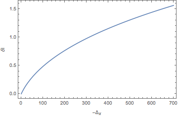
Likewise, we can substitute in the general expressions above and obtain the solution in terms of elliptic integrals (see Appendix for details). The function [see eq. (27)] is plotted in Fig. 1. One can also expand to any desired order in :
| (30) |
Terms up to agree with the previously known result (10). Note that this is the lightcone limit of the small temperature expansion of the correlator (in the large volume limit where is the temperature, is a theory-dependent numerical coefficient, and factors of have explicitly canceled out).
5. Discussion: We have computed the near lightcone behavior of HHLL correlators in CFTs with a large central charge in the large limit. The result provides a close analog of the Virasoro vacuum block in large- two-dimensional CFTs. It would be nice to see if the result could be simplified further (while we do have an expression in terms of the Appell functions/elliptic integrals, it is still a bit involved). Perhaps this would allow understanding of the algebraic structure behind the near-lightcone correlators (see Huang 2019; Huang 2020 for recent work in this direction).
We have explicitly matched the expansion of the length of the near-null geodesic to the near lightcone behavior of the correlator in the large and large limit. Note that one can read off the OPE coefficients from the exponential of . For example, the second term in the right-hand side of (10) determines the OPE coefficient of the two scalars with the stress-tensor and the leading [] behavior of the OPE coefficients of s with the leading twist -stress tensor operator .
One may ask whether the full correlator is well approximated by its stress-tensor sector. Generally we expect the multi trace operators of the form , to contribute. In the case, such contributions vanish in the large limit and the HHLL Virasoro vacuum block agrees with the full thermal correlator in the high temperature limit (in this limit the correlator can be computed by using a conformal transformation from to ). The situation in higher dimensions is more intricate (see e.g. Fitzpatrick and Huang 2019 for a recent discussion) 33 3 Note that multi stress tensor operators with any derivatives in them do not contribute in the large limit.. Nevertheless, in the large limit, multi-trace operators involving become heavy and decouple even for finite . Hence, in the large limit the stress tensor sector is a good approximation to the thermal correlator.
The results of Section 4 make it evident that as approaches a certain critical value, the spacelike geodesic gets closer to the horizon (this corresponds to the limit; similar behavior of geodesics was recently studied in Bianchi et al. 2020). It would be interesting to investigate this limit from the CFT point of view. It would also be interesting to relate our results to the behavior of quasinormal modes in the UV region Brigante et al. 2008a; Brigante et al. 2008b which is relevant for the conformal collider bounds Hofman and Maldacena 2008.
Other natural directions include explicit computations for finite (this would involve keeping the hypergeometric functions in (10) ) and generalization for finite values of . Also note that the universality of the multi stress tensor OPE coefficients may have a wider region of applicability than just the set of holographic theories. In this case the holographic calculation of this paper will have a wider regime of applicability as well.
Acknowledgements: I benefited from discussions with R. Karlsson, M. Kulaxizi, G.S. Ng, K. Sen and P. Tadić. This work was supported in part by an Irish Research Council Consolidator Laureate Award.
References
- Kulaxizi et al. (2019a) M. Kulaxizi, G. S. Ng, and A. Parnachev, SciPost Phys. 6, 065 (2019a), arXiv:1812.03120 [hep-th] .
- Fitzpatrick and Huang (2019) A. L. Fitzpatrick and K.-W. Huang, JHEP 08, 138 (2019), arXiv:1903.05306 [hep-th] .
- Karlsson et al. (2019) R. Karlsson, M. Kulaxizi, A. Parnachev, and P. Tadić, JHEP 10, 046 (2019), arXiv:1904.00060 [hep-th] .
- Li et al. (2019) Y.-Z. Li, Z.-F. Mai, and H. Lu, JHEP 09, 001 (2019), arXiv:1905.09302 [hep-th] .
- Kulaxizi et al. (2019b) M. Kulaxizi, G. S. Ng, and A. Parnachev, JHEP 10, 107 (2019b), arXiv:1907.00867 [hep-th] .
- Fitzpatrick et al. (2019) A. L. Fitzpatrick, K.-W. Huang, and D. Li, JHEP 11, 139 (2019), arXiv:1907.10810 [hep-th] .
- Karlsson et al. (2020a) R. Karlsson, M. Kulaxizi, A. Parnachev, and P. Tadić, JHEP 01, 076 (2020a), arXiv:1909.05775 [hep-th] .
- Li (2019) Y.-Z. Li, (2019), arXiv:1910.06357 [hep-th] .
- Karlsson (2019) R. Karlsson, (2019), arXiv:1912.01577 [hep-th] .
- Karlsson et al. (2020b) R. Karlsson, M. Kulaxizi, A. Parnachev, and P. Tadić, (2020b), arXiv:2002.12254 [hep-th] .
- Li and Zhang (2020) Y.-Z. Li and H.-Y. Zhang, (2020), arXiv:2004.04758 [hep-th] .
- Maldacena (1999) J. M. Maldacena, Int. J. Theor. Phys. 38, 1113 (1999), [Adv. Theor. Math. Phys.2,231(1998)], arXiv:hep-th/9711200 [hep-th] .
- Witten (1998a) E. Witten, Adv. Theor. Math. Phys. 2, 253 (1998a), arXiv:hep-th/9802150 [hep-th] .
- Gubser et al. (1998) S. S. Gubser, I. R. Klebanov, and A. M. Polyakov, Phys. Lett. B428, 105 (1998), arXiv:hep-th/9802109 [hep-th] .
- Witten (1998b) E. Witten, Adv. Theor. Math. Phys. 2, 505 (1998b), arXiv:hep-th/9803131 .
- Lashkari et al. (2018a) N. Lashkari, A. Dymarsky, and H. Liu, J. Stat. Mech. 1803, 033101 (2018a), arXiv:1610.00302 [hep-th] .
- Lashkari et al. (2018b) N. Lashkari, A. Dymarsky, and H. Liu, JHEP 03, 070 (2018b), arXiv:1710.10458 [hep-th] .
- Dymarsky and Pavlenko (2019) A. Dymarsky and K. Pavlenko, Phys. Rev. Lett. 123, 111602 (2019), arXiv:1903.03559 [hep-th] .
- (19) As explained in Section 2, is the separation between the insertions of the light operators in the rescaled lightlike direction.
- Fitzpatrick et al. (2013) A. Fitzpatrick, J. Kaplan, D. Poland, and D. Simmons-Duffin, JHEP 12, 004 (2013), arXiv:1212.3616 [hep-th] .
- Komargodski and Zhiboedov (2013) Z. Komargodski and A. Zhiboedov, JHEP 11, 140 (2013), arXiv:1212.4103 [hep-th] .
- Fitzpatrick et al. (2014) A. L. Fitzpatrick, J. Kaplan, and M. T. Walters, JHEP 08, 145 (2014), arXiv:1403.6829 [hep-th] .
- Fitzpatrick et al. (2015) A. L. Fitzpatrick, J. Kaplan, and M. T. Walters, JHEP 11, 200 (2015), arXiv:1501.05315 [hep-th] .
- Hijano et al. (2015a) E. Hijano, P. Kraus, and R. Snively, JHEP 07, 131 (2015a), arXiv:1501.02260 [hep-th] .
- Hijano et al. (2015b) E. Hijano, P. Kraus, E. Perlmutter, and R. Snively, JHEP 12, 077 (2015b), arXiv:1508.04987 [hep-th] .
- Fitzpatrick et al. (2016) A. L. Fitzpatrick, J. Kaplan, M. T. Walters, and J. Wang, JHEP 05, 069 (2016), arXiv:1510.00014 [hep-th] .
- Cotler and Jensen (2019) J. Cotler and K. Jensen, JHEP 02, 079 (2019), arXiv:1808.03263 [hep-th] .
- Collier et al. (2018) S. Collier, Y. Gobeil, H. Maxfield, and E. Perlmutter, (2018), arXiv:1811.05710 [hep-th] .
- Maxfield (2017) H. Maxfield, (2017), arXiv:1712.00885 [hep-th] .
- (30) In the following we mostly consider , but the limit can also be recovered.
- Huang (2019) K.-W. Huang, Phys. Rev. D 100, 061701 (2019), arXiv:1907.00599 [hep-th] .
- Huang (2020) K.-W. Huang, (2020), arXiv:2002.00110 [hep-th] .
- (33) Note that multi stress tensor operators with any derivatives in them do not contribute in the large limit.
- Bianchi et al. (2020) M. Bianchi, A. Grillo, and J. F. Morales, (2020), arXiv:2002.05574 [hep-th] .
- Brigante et al. (2008a) M. Brigante, H. Liu, R. C. Myers, S. Shenker, and S. Yaida, Phys. Rev. D 77, 126006 (2008a), arXiv:0712.0805 [hep-th] .
- Brigante et al. (2008b) M. Brigante, H. Liu, R. C. Myers, S. Shenker, and S. Yaida, Phys. Rev. Lett. 100, 191601 (2008b), arXiv:0802.3318 [hep-th] .
- Hofman and Maldacena (2008) D. M. Hofman and J. Maldacena, JHEP 05, 012 (2008), arXiv:0803.1467 [hep-th] .
Supplemental Material
Appendix A A. Details of the case
Appendix B B. Details of the case
The integrals can be rewritten in terms of special functions. For example,
| (33) |
where , are the (-dependent) roots of the polynomial in the decreasing order and is the Appel function. Likewise,
| (34) |
It will be convenient to parameterize the solutions in terms of a new variable, . One can derive the following expressions:
| (35) |
Hence, eq. (28) becomes
| (36) |
where . We generally need to invert this, which is a simple exercise perturbatively,
| (37) |
To deal with the divergence, one can differentiate in (25) with respect to . This makes the integral convergent and kills the term, but one would need to integrate back with respect to to recover the result:
| (38) |
where and and are given by (33), (34) and and are related to by (35), while is given by
| (39) |
Eq. (39) can be expanded perturbatively in ,
| (40) |
where we omit a constant term. Substituting eq. (40) into eq. (38) yields eq. (30).