Detection and Isolation of Wheelset Intermittent Over-creeps for Electric Multiple Units Based on a Weighted Moving Average Technique

The creep phenomenon can be defined as a wheel-rail micro-elastic slide through relative deformation [11]. As shown in Fig. 1, since both the wheel and rail are elastic bodies, a normal load $F_{g}$ leads to local micro-elastic deformation at their contact point. Then, an area of contact (i.e., the contact patch) is formed. As a result, when a tractive torque $T_{w}$ or braking torque is applied, pure rolling rarely takes place and a slight slide arises between the wheel and rail, called creep. The creep causes a small difference between the forward velocity $v_{t}$ and wheel circumference line velocity $v$. This relative difference is called creep velocity $v_{c}$ and is given by

The adhesion coefficient $\eta$, which is defined as the ratio between adhesion force $F_{ad}$ and normal load $F_{g}$ as follows,

has a close relation to $v_{c}$ when the WR surface condition is constant. Generally speaking, a dry, clean WR surface generates a higher $\eta$ compared with a wet surface. $\eta$ can be further reduced on an oily surface. The $\eta-v_{c}$ relationships, i.e., adhesion characteristic curves (ACCs), with various WR surface conditions were shown in [14, 11]. ACCs rise first and then decline. Hence, each ACC has its own peak point $v^{*}_{c}$, where the adhesion force $F_{ad}$ reaches a maximum $F_{ad}(v^{*}_{c})=\eta(v^{*}_{c})F_{g}$. It can be seen that a proper creep velocity is beneficial to generate the adhesion force, and thus, the creep velocity should be controlled within a certain range to track a high adhesion point [11]. While appropriate creep is desired, over-creep has several disadvantages, such as reduction in adhesion force and additional wear to WRs.

There are two kinds of over-creep phenomena, namely, slip and slide. Since tractive torque $T_{w}$ is equivalent to the moment of a couple $F_{w}$, we now use $F_{w}$ instead of $T_{w}$ in Fig. 1. It can be seen that $F_{w}$ acting on the contact patch is resisted by a force of friction called adhesion force $F_{ad}$. When $F_{w}$ is less than the maximum available adhesion force $F_{ad}(v^{*}_{c})$, their resultant is zero and the remained $F_{w}$ acting on the wheelset mass center accelerates the EMU. However, when $F_{w}$ exceeds $F_{ad}(v^{*}_{c})$, their resultant cannot be zero, resulting in a toque $T_{c}=(F_{w}-F_{ad})r$ that rotates the wheelset. In this way, slip takes place and the wheelset accelerates abnormally. Similarly, when the equivalent couple generated by a braking torque exceeds the maximum available adhesion force, slide takes place and the wheelset decelerates abnormally. The result is that the velocity of the slipping (sliding) wheelset becomes greater (lower) than that of other normal wheelsets.

The fact that ACCs rise first and then decline is due to structural changes of the contact patch. When the WRs have smooth surfaces and constant curvature in the vicinity of the contact patch, the contact patch is believed to be elliptical in shape, and divided into adhesion area and slip/slide area [8]. The adhesion area, in which the surfaces are locked together, locates at the front of the contact patch. It reduces progressively as the adhesion force increases. When only the slip/slide area is left, the adhesion between wheel and rail breaks down, leading to the decline in the ACC.

Typically, one EMU car has four wheelsets, each equipped with a speed sensor. Thus, a total of four channels of wheelset velocity $\{v_{i},i=1\thicksim 4\}$ are measured and utilized by the ASS system. Denote the velocity and acceleration of the $i$th wheelset as $v_{i}$ and $a_{i}=\dot{v}_{i}$, respectively. Note that $v_{t}$ is not directly measurable, so currently used ASS strategies are generally based on the wheelset velocity difference and wheelset acceleration as follows.

Velocity information plays an important role in the DI of over-creeps. In practice, speed sensors are equipped on bogies, which are in direct contact with rails. As a result, speed sensors are susceptible to noises and disturbances caused by the harsh working environment (e.g., vibration, shock, electromagnetic interference, severe weather). Therefore, modern EMUs must have robust and advanced ASS systems. Although current strategies fully consider the creep mechanisms and consequently can ensure the safe operation of EMUs, their efficiency for WIOs that have small magnitude and short duration remains to be improved. Therefore, the objective of this paper is to improve the DI performance of WIOs using only the velocity measurements $v_{i}$. The DI of a WIO means that slip and slide should be detected and distinguished from each other. Moreover, its location, namely, which wheelsets it occurs on, should be determined.

Without loss of generality, we assume that there are $p$ channels of measurement available $\{v_{i},i=1\thicksim p\}$. For a sample vector $\mathbf{v}=[v_{1},v_{2},\cdots,v_{p}]^{T}\in{\mathbb{R}}^{p}$, its variable-to-minimum difference (VMD) index for the $i$th variable is defined as

According to (3), the $\textrm{VMD}_{i}(\mathbf{v})$ index can be used to detect and isolate the $i$th wheelset’s slip in traction mode. Moreover, following

we have

Then, according to (4), the $\textrm{VMD}_{i}(\mathbf{-v})$ index can be used to detect and isolate the $i$th wheelset’s slide in braking mode.

The mechanism is readily comprehensible. It can be seen from equation (1) that a wheelset’s absolute velocity equals the train velocity plus its creep velocity. Since all the wheelsets on the same EMU car are controlled by one traction control unit (TCU) and are of the same type and size, they provide almost equal adhesion force under normal conditions. Considering the EMU’s mass is distributed nearly equally on each wheelset whose WR surface conditions are the same, according to (2), the creep velocities and consequently the absolute velocities of these wheelsets should be quite similar. To illustrate this point intuitively, the velocity values of four wheelsets are collected from a practical EMU car under normal conditions and are shown in Fig. 2. For clarity, only a part of the samples are displayed. This EMU, or specifically, this URT, has made two stops in five minutes. A zero wheelset velocity means that the train has arrived at a station. The inter-station run of URTs usually contains three modes, namely, traction, coasting and braking. It can be observed that the wheelset velocities are almost the same throughout the three modes.

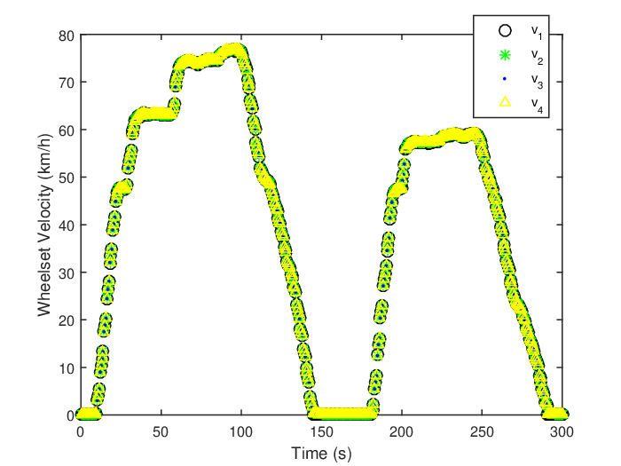
For a sample vector $\mathbf{v}$, the $\textrm{VMD}_{i}$ index measures the degree of difference between its $i$th variable and its minimum variable. Since these variables should be consistent with each other under normal conditions, all $p$ VMD indices of a normal sample vector should be small. A large $\textrm{VMD}_{i}(\mathbf{v})$ indicates potential IOs of the $i$th wheelset. This, combined with the diagnosis logic that slip (slide) can only happen in traction (braking) mode, helps us discriminate slip from slide.

The VMD index is applicable to cases where the measurement variables are similar to each other under normal conditions. Note that this kind of situation holds for many practical systems such as brake cylinder systems [2], air brake systems [29] and bearing systems [30] of EMUs. Moreover, when this application condition is satisfied, the VMD index has several advantages. First, by using the VMD index, a non-stationary process is transformed into a stationary process, which is easier to be monitored. Second, the DI task can be accomplished by the VMD index in one step because of its clear and readily comprehensible diagnosis logic. Third, $\textrm{VMD}_{i}(\mathbf{v})$ is unidimensional and thus easy to be implemented online. Note that it should not be considered as an univariate monitoring strategy because $\textrm{VMD}_{i}(\mathbf{v})$ makes use of multidimensional measurement. To utilize the VMD index, we collect $N$ training samples $\{\mathbf{v}_{k},k=1,2,\cdots,N\}$ under normal conditions. For online DI, we collect new measurement $\mathbf{v}^{f}_{k}$ in real time.

The moving average (MA) is a widely known method to improve the robustness and sensitivity. By employing a sliding time window, disturbance is filtered and detectability is improved [31, 32, 33, 34, 35, 36]. However, the optimality of its equally weighted scheme remains unproven. Take the least squares (LS) technique as an example. Compared with the standard LS technique, the weighted LS technique often achieves better performance when the weights are properly selected. Therefore, in this paper, we construct a weighted moving average VMD (WMA-VMD) index, which is given as follows:

where $\mathbf{a}_{W}=[a_{1},a_{2},\cdots,a_{W}]^{T}$ is a weight vector. For the WMA-VMD index, we put different weights on samples in the time window, as shown in (III-B).

The WMA-VMD index for training data is then

In practice, $\{\textrm{VMD}_{i}(\mathbf{v}_{k}),k=1,2,\cdots,N\}$ can be viewed as a stationary process. That is, for all $k$, ${\mathbb{E}}\left\{\textrm{VMD}_{i}(\mathbf{v}_{k})\right\}=\mu_{i}$ and the autocorrelation function ${\mathbb{C}\rm{ov}}\left\{\textrm{VMD}_{i}(\mathbf{v}_{k}),\textrm{VMD}_{i}(\mathbf{v}_{k-l})\right\}=R_{i,l}$ depends only on the lag $l$. Then, we can derive the statistical properties of the WMA-VMD index as follows:

However, parameters $\mu_{i},R_{i,l},\tilde{S}_{i}(\mathbf{a}_{W})$ are unknown. According to the estimation theory of the mean and the auto-covariance function of the stationary process [37], we can estimate them as follows:

For the WMA-VMD index, the weight vector is a crucial parameter that can directly affect the DI performance of WIOs. It can be seen from (III-B) that the mean of WMA-VMD index is constant while its variance depends on the weight vector. Thus, the OWV should minimize the variance. The problem formulation is given as follows.

Proof. Let $\epsilon_{j}=\textrm{VMD}_{i}(\mathbf{v}_{j})-\hat{\mu}_{i},\ j=1,\cdots,N$. Then, we can rewrite $\hat{\mathbf{\Gamma}}^{k}_{i}=\frac{1}{N}\mathbf{\Upsilon}\mathbf{\Upsilon}^{T}$, where $\mathbf{\Upsilon}\in{\mathbb{R}}^{k\times(N+k-1)}$ and

Thus, $\hat{\mathbf{\Gamma}}^{k}_{i}$ is positive semidefinite. Moreover, $\mathbf{\Upsilon}$ is nonsingular if and only if there is at least one nonzero $\epsilon_{j}$, which is equivalent to $\hat{R}_{i,0}>0$.

Proof. Since this is a constrained optimization problem, we construct a Lagrange function as follows:

where $\lambda$ is a Lagrange multiplier. Note that

where the last inequality is because of Lemma 1. Thus, Problem 1 is a convex optimization. Then, a weight vector $\mathbf{a}^{*}_{W}$ minimizes $\hat{S}_{i}(\mathbf{a}_{W})$ of Problem 1 if and only if it satisfies the Karush-Kuhn-Tucker conditions [38], i.e., $\nabla_{\mathbf{a}_{W}}{\cal L}(\mathbf{a}_{W},\lambda)=\mathbf{0}_{W},\ \nabla_{\lambda}{\cal L}(\mathbf{a}_{W},\lambda)=0$. By setting the derivative of ${\cal L}(\mathbf{a}_{W},\lambda)$ with respect to $\mathbf{a}_{W}$ to zeros, we obtain

Integrating (23) with (14), we derive $\hat{\mathbf{A}}\mathbf{a}^{*}_{W}=\mathbf{b}$.

Now, we prove that $\hat{\mathbf{A}}$ is nonsingular so that the OWV is unique. By following a few reformulations, we can rewrite $\hat{\mathbf{A}}=\hat{\mathbf{J}}\hat{\mathbf{\Gamma}}^{W}_{i}$, where

For $|\hat{\mathbf{J}}|$, adding its $j$th column to its $j\!-\!1$th column in turn, we obtain $|\hat{\mathbf{J}}|=\mathbf{1}^{T}_{W}(\hat{\mathbf{\Gamma}}^{W}_{i})^{-1}\mathbf{1}_{W}>0$. Thus, $\hat{\mathbf{A}}$ is nonsingular and the proof is complete.

Proof. It can be seen from (1) that

Denote $\hat{\mathbf{A}}_{\backslash l\backslash\emptyset}$ and $\hat{\mathbf{A}}_{\backslash\emptyset\backslash j}$ as the matrices obtained from $\hat{\mathbf{A}}$ by deleting the $l$th row and the $j$th column, respectively. Then, $\hat{\mathbf{A}}_{\backslash W\backslash\emptyset}\in{\mathbb{R}}^{(W-1)\times W}$ has the following form:

where $t_{l}=\hat{R}_{i,l}-\hat{R}_{i,l-1}$. Define $\textrm{cen}(\mathbf{A})\in{\mathbb{R}}^{p\times q}$ as the centrosymmetry of a matrix $\mathbf{A}\in{\mathbb{R}}^{p\times q}$, namely, $[\textrm{cen}(\mathbf{A})]_{l,j}\!=\![\mathbf{A}]_{p-l+1,q-j+1}$. It can be easily verified that

Besides, if $\mathbf{A}$ is a square matrix, then we have $|\textrm{cen}(\mathbf{A})|=|\mathbf{A}|$. Moreover, if $\mathbf{A}$ is centrosymmetric, that is to say, $\textrm{cen}(\mathbf{A})=\mathbf{A}$, we have

As for $\hat{\mathbf{A}}$, note that $[\hat{\mathbf{A}}_{\backslash W\backslash\emptyset}]_{l,j}\!=\!-[\hat{\mathbf{A}}_{\backslash W\backslash\emptyset}]_{W-l,W-j+1}$, i.e., $\textrm{cen}(\hat{\mathbf{A}}_{\backslash W\backslash\emptyset})\!=\!-\hat{\mathbf{A}}_{\backslash W\backslash\emptyset}$. According to (25) and (26), we have

Thus,

Note that $\mathbf{a}^{*}_{W}=\hat{\mathbf{A}}^{-1}\mathbf{b}=|\hat{\mathbf{A}}|^{-1}\textrm{adj}(\hat{\mathbf{A}})\mathbf{b}$. Then,

which completes the proof.

Proof. Directly derived from Theorems 1 and 2.

Proof. When the process data are independent, we have $\hat{R}_{i,l}=0$, $\forall l\neq 0$. Thus, in this case, we have

and

According to (28), $a^{*}_{m}=(-1)^{W+m}|\hat{\mathbf{A}}|^{-1}\left|\hat{\mathbf{A}}_{\backslash W\backslash m}\right|=1/W$.

Proof. According to (19) and the Cramer’s rule, we have

where $\hat{\mathbf{B}}^{m}$ is the matrix obtained by replacing the $m$th column of $\hat{\mathbf{A}}$ by $\mathbf{b}$. By following the properties of determinants, we have $|\hat{\mathbf{B}}^{m}|\!=\!|\check{\mathbf{A}}^{m}|$, where $\delta_{mj}$ is the Kronecker function and

Moreover, by following a few reformulations, we can rewrite $\check{\mathbf{A}}^{m}=\check{\mathbf{J}}^{m}\hat{\mathbf{\Gamma}}^{W}_{i}$, where

For $|\check{\mathbf{J}}^{m}|$, adding its $j$th column to its $j\!-\!1$th column in turn, we obtain $|\check{\mathbf{J}}^{m}|=\mathbf{e}^{T}_{Wm}(\hat{\mathbf{\Gamma}}^{W}_{i})^{-1}\mathbf{1}_{W}$. Then,

Recall that $|\hat{\mathbf{J}}|=\mathbf{1}^{T}_{W}(\hat{\mathbf{\Gamma}}^{W}_{i})^{-1}\mathbf{1}_{W}>0$. Thus, we have $a^{*}_{m}>(=,<)0$ if and only if $|\check{\mathbf{J}}^{m}|=\mathbf{e}^{T}_{Wm}(\hat{\mathbf{\Gamma}}^{W}_{i})^{-1}\mathbf{1}_{W}>(=,<)0$, which is further equivalent to

where $\hat{\mathbf{M}}^{W}_{i}$ is the adjoint of $\hat{\mathbf{\Gamma}}^{W}_{i}$. Note that $[\hat{M}^{W}_{i}]_{l,j}$ is the algebraic cofactor of $[\hat{\Gamma}^{W}_{i}]_{j,l}$. Thus, we have

which completes the proof.

In traction mode, the $i$th wheelset’s creep is considered normal at time instance $k$, if $\widetilde{\textrm{VMD}}_{i,k}(\mathbf{a}^{*}_{W},\mathbf{v}^{f})\leq\delta_{i,W}$. Otherwise, the $i$th wheelset is considered to be slipping. The control limit (CL) $\delta_{i,W}$ can be determined based on the historical data as follows:

In braking mode, the procedure is the same except that we should use $-\mathbf{v},-\mathbf{v}^{f}$ instead of $\mathbf{v},\mathbf{v}^{f}$ in all of the above steps. Overall, the DI algorithm of WIOs based on the WMA-VMD index with window length $W$ is summarized as Algorithm 1.

In this subsection, important properties, such as the triangle inequality, of the VMD operator are proven, see Theorem 5. We begin with the proof of some properties of the $\min$ operator.

Proof. Equalities (39) and (40) are obvious. As for inequality (41), its left side has four possible values, i.e.,

As for the right side of inequality (41), we have

Moreover, when $a\leq b,d\leq c$, the right side of inequality (41) has two possible values, i.e.,

It can be easily seen that both of them are no less than $a+d$ since $a\leq b,d\leq c$. Similarly, when $b\leq a,c\leq d$, the right side of inequality (41) also has these two possible values, both of which are no less than $b+c$ since $b\leq a,c\leq d$. Based on the above discussions, we obtain (41). Furthermore, following the above proof, we can conclude that the equality in (41) holds if and only if at least one of the following conditions is satisfied:

The above conditions can be simplified as

References

- [1] H. T. Chen, B. Jiang, N. Y. Lu, and Z. H. Mao, “Deep pca based real-time incipient fault detection and diagnosis methodology for electrical drive in high-speed trains,” IEEE Transactions on Vehicular Technology, vol. 67, no. 6, pp. 4819–4830, 2018.
- [2] D. H. Zhou, H. Q. Ji, X. He, and J. Shang, “Fault detection and isolation of the brake cylinder system for electric multiple units,” IEEE Transactions on Control Systems Technology, vol. 26, no. 5, pp. 1744–1757, 2018.
- [3] H. T. Chen, B. Jiang, and S. X. Ding, “A broad learning aided data-driven framework of fast fault diagnosis for high-speed trains,” IEEE Intelligent Transportation Systems Magazine, Published online, DOI: 10.1109/MITS.2019.2907629.
- [4] S. Kadowaki, K. Ohishi, T. Hata, N. Iida, M. Takagi, T. Sano, and S. Yasukawa, “Antislip readhesion control based on speed-sensorless vector control and disturbance observer for electric commuter train - Series 205-5000 of the East Japan Railway Company,” IEEE Transactions on Industrial Electronics, vol. 54, no. 4, pp. 2001–2008, 2007.
- [5] K. Ohishi, T. Hata, T. Sano, and S. Yasukawa, “Realization of anti-slip/skid re-adhesion control for electric commuter train based on disturbance observer,” IEEJ Transactions on Electrical and Electronic Engineering, vol. 4, no. 2, pp. 199–209, 2009.
- [6] S. Q. Zheng and M. E. Kahn, “China’s bullet trains facilitate market integration and mitigate the cost of megacity growth,” Proceedings of the National Academy of Sciences, vol. 110, no. 14, pp. E1248–E1253, 2013.
- [7] H. T. Chen and B. Jiang, “A review of fault detection and diagnosis for the traction system in high-speed trains,” IEEE Transactions on Intelligent Transportation Systems, Published online, DOI: 10.1109/TITS.2019.2897583.
- [8] A. H. Wickens, Fundamentals of Rail Vehicle Dynamics Guidance and Stability. Lisse, Netherlands: Swets & Zeitlinger, 2003.
- [9] S. Iwnicki, Handbook of Railway Vehicle Dynamics. CRC press, 2006.
- [10] K. Knothe and S. Stichel, Rail Vehicle Dynamics. Springer, 2017.
- [11] L. J. Diao, L. T. Zhao, Z. M. Jin, L. Wang, and S. M. Sharkh, “Taking traction control to task: High-adhesion-point tracking based on a disturbance observer in railway vehicles,” IEEE Industrial Electronics Magazine, vol. 11, no. 1, pp. 51–62, 2017.
- [12] D. H. Zhou, Y. H. Zhao, Z. D. Wang, X. He, and M. Gao, “Review on diagnosis techniques for intermittent faults in dynamic systems,” IEEE Transactions on Industrial Electronics, vol. 67, no. 3, pp. 2337–2347, 2020.
- [13] S. G. Zhang, Fundamental Application Theory and Engineering Technology for Railway High-speed Trains. Beijing, China: Science Press, 2007.
- [14] S. Wang, J. Xiao, J. C. Huang, and H. M. Sheng, “Locomotive wheel slip detection based on multi-rate state identification of motor load torque,” Journal of the Franklin Institute, vol. 353, no. 2, pp. 521–540, 2016.
- [15] T. X. Mei, J. H. Yu, and D. A. Wilson, “A mechatronic approach for effective wheel slip control in railway traction,” Proceedings of the Institution of Mechanical Engineers, Part F: Journal of Rail and Rapid Transit, vol. 223, no. 3, pp. 295–304, 2009.
- [16] K. Kim, S. H. Kong, and S. Y. Jeon, “Slip and slide detection and adaptive information sharing algorithms for high-speed train navigation systems,” IEEE Transactions on Intelligent Transportation Systems, vol. 16, no. 6, pp. 3193–3203, 2015.
- [17] M. Spiryagin, K. S. Lee, and H. H. Yoo, “Control system for maximum use of adhesive forces of a railway vehicle in a tractive mode,” Mechanical systems and signal processing, vol. 22, no. 3, pp. 709–720, 2008.
- [18] P. V. Tu, Q. L. Bao, L. Zhang, H. G. Xu, and Y. D. Du, “A fuzzy adaptive reasoning method for trains slide/slip detection,” in 14th International Computer Conference on Wavelet Active Media Technology and Information Processing (ICCWAMTIP), Chengdu, China, pp. 1–4. IEEE, 2017.
- [19] B. G. Cai, J. Wang, Q. Yin, and J. Liu, “A GNSS based slide and slip detection method for train positioning,” in 2009 Asia-Pacific Conference on Information Processing, vol. 1, pp. 450–453. IEEE, 2009.
- [20] T. Watanabe and M. Yamashita, “Basic study of anti-slip control without speed sensor for multiple motor drive of electric railway vehicles,” in Proceedings of the Power Conversion Conference, Osaka, Japan, vol. 3, pp. 1026–1032, 2002.
- [21] M. Yamashita and T. Watanabe, “Readhesion control method without speed sensors for electric railway vehicles,” Quarterly Report of RTRI, vol. 46, no. 2, pp. 85–89, 2005.
- [22] S. S. Saab, G. E. Nasr, and E. A. Badr, “Compensation of axle-generator errors due to wheel slip and slide,” IEEE Transactions on Vehicular Technology, vol. 51, no. 3, pp. 577–587, 2002.
- [23] M. A. Çimen, Ö. Ararat, and M. T. Söylemez, “A new adaptive slip-slide control system for railway vehicles,” Mechanical Systems and Signal Processing, vol. 111, pp. 265–284, 2018.
- [24] J. Xiao, H. Weiss, and H. Wang, “Locomotive optimal adhesion control by wavelet analysis,” in IEEE International Conference on Industrial Technology, Maribor, Slovenia, vol. 1, pp. 309–314. IEEE, 2003.
- [25] J. C. Huang, J. Xiao, Y. F. Bai, and S. Q. Liao, “Optimized adhesion control of electric locomotives based on wavelet analysis and cloud model,” in International Conference on Transportation Engineering, pp. 3209–3214, 2007.
- [26] I. Yasuoka, T. Henmi, Y. Nakazawa, and I. Aoyama, “Improvement of re-adhesion for commuter trains with vector control traction inverter,” in Proceedings of Power Conversion Conference, Nagaoka, Japan, vol. 1, pp. 51–56. IEEE, 1997.
- [27] G. Niu, L. J. Xiong, X. X. Qin, and M. Pecht, “Fault detection isolation and diagnosis of multi-axle speed sensors for high-speed trains,” Mechanical Systems and Signal Processing, vol. 131, pp. 183–198, 2019.
- [28] Z. H. Mao, X. G. Yan, B. Jiang, and M. Chen, “Adaptive fault-tolerant sliding-mode control for high-speed trains with actuator faults and uncertainties,” IEEE Transactions on Intelligent Transportation Systems, Published online, DOI: 10.1109/TITS.2019.2918543.
- [29] T. X. Guo, D. H. Zhou, J. F. Zhang, M. Y. Chen, and X. H. Tai, “Fault detection based on robust characteristic dimensionality reduction,” Control Engineering Practice, vol. 84, pp. 125–138, 2019.
- [30] T. Fang, Q. Liu, and D. L. Cui, “Multi-direction reconstruction for fault diagnosis of train bearings,” in International Conference on Intelligent Rail Transportation, Singapore, 2018.
- [31] J. H. Chen, C. M. Liao, F. R. J. Lin, and M. J. Lu, “Principle component analysis based control charts with memory effect for process monitoring,” Industrial & Engineering Chemistry Research, vol. 40, no. 6, pp. 1516–1527, 2001.
- [32] H. Q. Ji, X. He, J. Shang, and D. H. Zhou, “Incipient sensor fault diagnosis using moving window reconstruction-based contribution,” Industrial & Engineering Chemistry Research, vol. 55, no. 10, pp. 2746–2759, 2016.
- [33] H. Q. Ji, X. He, J. Shang, and D. H. Zhou, “Incipient fault detection with smoothing techniques in statistical process monitoring,” Control Engineering Practice, vol. 62, pp. 11–21, 2017.
- [34] H. T. Chen, B. Jiang, W. Chen, and H. Yi, “Data-driven detection and diagnosis of incipient faults in electrical drives of high-speed trains,” IEEE Transactions on Industrial Electronics, vol. 66, no. 6, pp. 4716–4725, 2019.
- [35] H. T. Chen, B. Jiang, and N. Y. Lu, “A newly robust fault detection and diagnosis method for high-speed trains,” IEEE Transactions on Intelligent Transportation Systems, vol. 20, no. 6, pp. 2198–2208, 2019.
- [36] J. X. Sang, J. F. Zhang, T. X. Guo, D. H. Zhou, M. Y. Chen, and X. H. Tai, “Detection of incipient faults in emu braking system based on data domain description and variable control limit,” Neurocomputing, vol. 383, pp. 348–358, 2020.
- [37] P. J. Brockwell and R. A. Davis, Time Series: Theory and Methods (2nd edition). Springer Science and Business Media, 1991.
- [38] D. G. Luenberger and Y. Ye, Linear and Nonlinear Programming (3rd edition). Springer Science and Business Media, 2008.
- [39] X. Y. Yang, C. H. Yang, T. Peng, Z. W. Chen, B. Liu, and W. H. Gui, “Hardware-in-the-loop fault injection for traction control system,” IEEE Journal of Emerging and Selected Topics in Power Electronics, vol. 6, no. 2, pp. 696–706, 2018.