跳到论文正文
W Papers独立论文阅读器 arXiv:2005.06372 论文正文 计算阅读时间 · 0%
引用这篇论文根据当前论文元数据生成,正式投稿前建议核对。


License: arXiv.org perpetual non-exclusive license
arXiv:2005.06372v2 [math.PR] 21 Aug 2020
 

Growth-fragmentation process embedded in a planar Brownian excursion

by

Elie Aïdékon11 1 LPSM, Sorbonne Université Paris VI, and Institut Universitaire de France, elie.aidekon@upmc.fr and William Da Silva22 2 LPSM, Sorbonne Université Paris VI, william.da-silva@lpsm.paris

Summary.

The aim of this paper is to present a self-similar growth-fragmentation process linked to a Brownian excursion in the upper half-plane ℍ\mathbb{H}, obtained by cutting the excursion at horizontal levels. We prove that the associated growth-fragmentation is related to one of the growth-fragmentation processes introduced by Bertoin, Budd, Curien and Kortchemski in [6].

Keywords. Growth-fragmentation process, self-similar Markov process, planar Brownian motion, excursion theory.

2010 Mathematics Subject Classification. 60D05.

1 Introduction

We consider a Brownian excursion in the upper half-plane ℍ\mathbb{H} from 00 to a positive real number z0z_{0}. For a>0a>0, if the excursion hits the set {z∈ℂ:ℑ⁡(z)=a}\{z\in\mathbb{C}\,:\,\Im(z)=a\} of points with imaginary part aa, it will make a countable number of excursions above it, that we denote by (eia,+,i≥1)(e_{i}^{a,+},\,i\geq 1). For any such excursion, we let Δ​eia,+\Delta e_{i}^{a,+} be the difference between the endpoint of the excursion and its starting point, which we will refer to as the size or length of the excursion. Since both points have the same imaginary part, the collection (Δ​eia,+,i≥1)(\Delta e_{i}^{a,+},\,i\geq 1) is a collection of real numbers and we suppose that they are ranked in decreasing order of their magnitude. Our main theorem describes the law of the process (Δ​eia,+,i≥1)a≥0(\Delta e_{i}^{a,+},\,i\geq 1)_{a\geq 0} indexed by aa in terms of a self-similar growth-fragmentation. We refer to [5] and [6] for background on growth-fragmentations. Let us describe the growth-fragmentation process involved in our case.

Let Z=(Za)0≤a<ζZ=(Z_{a})_{0\leq a<\zeta} be the positive self-similar Markov process of index 11 whose Lamperti representation is

Za=z0​exp⁡(ξ⁡(τ⁡(z0−1​a))),Z_{a}=z_{0}\exp(\xi(\tau(z_{0}^{-1}a))),

where ξ\xi is the Lévy process with Laplace exponent

Ψ⁡(q)=−4π​q+2π​∫y>−ln⁡(2)(eq​y−1−q⁡(ey−1))​e−y​d​y(ey−1)2,q<3,\Psi(q)=-\frac{4}{\pi}q+\frac{2}{\pi}\int_{y>-\ln(2)}\left(\mathrm{e}^{qy}-1-q(\mathrm{e}^{y}-1)\right)\frac{\mathrm{e}^{-y}\mathrm{d}y}{(\mathrm{e}^{y}-1)^{2}},\quad q<3, (1)

τ\tau is the time change

τ(a)=inf{s≥0,∫0seξ⁡(u)du>a},\tau(a)=\inf\left\{s\geq 0,\;\int_{0}^{s}\mathrm{e}^{\xi(u)}\mathrm{d}u>a\right\},

and ζ=inf{a≥0,Za=0}\zeta=\inf\{a\geq 0,\;Z_{a}=0\}. The cell system driven by ZZ can be roughly constructed as follows. The size of the so-called Eve cell is z0z_{0} at time 00 and evolves according to ZZ. Then, conditionally on ZZ, we start at times aa when a jump Δ​Za=Za−Za−\Delta Z_{a}=Z_{a}-Z_{a-} occurs independent processes starting from −Δ​Za-\Delta Z_{a}, distributed as ZZ when Δ​Za<0\Delta Z_{a}<0 and as −Z-Z when Δ​Za>0\Delta Z_{a}>0. These processes represent the sizes of the daughters of the Eve particle. Then repeat the process for all the daughter cells: at each jump time of the cell process, start an independent copy of the process ZZ if the jump is negative, −Z-Z if the jump is positive, with initial value the negative of the corresponding jump. This defines the sizes of the cells of the next generation and we proceed likewise. We then define, for a≥0a\geq 0, 𝐗¯​(a)\overline{\mathbf{X}}(a) as the collection of sizes of cells alive at time aa, ranked in decreasing order of their magnitude.

Growth-fragmentation processes were introduced in [5]. Beware that the growth-fragmentation process we just defined is not included in the framework of [5] or [6] because we allow cells to be created at times corresponding to positive jumps, giving birth to cells with negative size. Therefore, the process 𝐗¯\overline{\mathbf{X}} is not a true growth-fragmentation process. The formal construction of the process 𝐗¯\overline{\mathbf{X}} is done in Section 4. The following theorem is the main result of the paper.

Theorem 1.1.

The process (Δ​eia,+,i≥1)a≥0(\Delta e_{i}^{a,+},\,i\geq 1)_{a\geq 0} is distributed as 𝐗¯\overline{\mathbf{X}}.

Remarks.

  • •

    The fact that there is no local explosion (in the sense that there is no compact of ℝ\{0}\mathbb{R}\backslash\{0\} with infinitely many elements of 𝐗¯\overline{\mathbf{X}}) can be seen as a consequence of the theorem.

  • •

    From the skew-product representation of planar Brownian motion, this theorem has an analog in the radial setting. It can be stated as follows. Take a Brownian excursion in the unit disc from boundary to boundary, with continuous determination of its argument (i.e., its winding number around the origin) z0>0z_{0}>0. Then, for each a≥0a\geq 0, record for each excursion made in the disc of radius e−a{\rm e}^{-a} the corresponding winding number. The collection of these winding numbers, ranked in decreasing order of their magnitude and indexed by aa is distributed as 𝐗¯\overline{\mathbf{X}}.

  • •

    One could finally look at the growth-fragmentation associated to the Brownian bubble measure in ℍ\mathbb{H}. It would give an infinite measure on the space of (signed) growth-fragmentation processes starting from 00. In the non-critical case (i.e. when the natural martingale associated to the intrinsic area converges in L1L^{1}), a measure on growth-fragmentation processes starting from 00 has been constructed by Bertoin, Curien and Kortchemski [7], see Section 4.3 there.

Related works. A pure fragmentation process was identified by Bertoin [4] in the case of the linear Brownian excursion where the size of an excursion was there its duration. Le Gall and Riera [16] identified a growth-fragmentation process in the Brownian motion indexed by the Brownian tree. We will follow the strategy of this paper, making use of excursion theory to prove our theorem.

When killing in 𝐗¯\overline{\mathbf{X}} all cells with negative size (and their progeny), one recovers a genuine self-similar (positive) growth-fragmentation driven by ZZ, call it 𝐗\mathbf{X}. The process 𝐗\mathbf{X} appears in the work of Bertoin et al. [6], compare Proposition 5.2 in [6] with Proposition 4.2 below. In Section 3.3 of [6], the authors exhibit remarkable martingales associated to growth-fragmentation processes and describe the corresponding changes of measure. In the case of 𝐗\mathbf{X}, the martingale consists in summing the sizes raised to the power 5/25/2 of all cells alive at time aa. Under the change of measure, the process 𝐗\mathbf{X} has a spinal decomposition: the size of the tagged particle is a Cauchy process conditioned on staying positive, while other cells behave normally. In the case of 𝐗¯\overline{\mathbf{X}}, where we also include cells with negative size, a similar martingale appears, substituting 22 for 5/25/2, while the tagged particle will now follow a Cauchy process (with no conditioning). It is the content of Section 3.3. This martingale is related to the one appearing in [2], where a change of measure was also specified. In that paper, the authors exhibit a martingale in the radial case, see Section 7.1 there. The martingale in our setting can be viewed as a limit case, where one conformally maps the unit disc to the upper half-plane, then sends the image of the origin towards infinity.

Connection with random planar maps. In [6], the authors relate a distinguished family of growth-fragmentation processes to the exploration of a Boltzmann planar map, see Proposition 6.6 there. The mass of a particle in the growth-fragmentation represents the perimeter of a region in the planar map which is currently explored, a negative jump the splitting of the region into two smaller regions to be explored, and a positive jump the discovery of a face with large degree. In this setting, only a negative jump is a birth event. The area of the map is identified as the limit of a natural martingale associated to the underlying branching random walk, see Corollary 6.7 there.

On the other hand, a Boltzmann random map can also be seen as the gasket of a O⁡(n)O(n) loop model, see Section 8 of [15]. From this point of view, a positive jump of the growth-fragmentation stands for the discovery of a loop which still has to be explored, so that positive jumps will be birth events too. The signed growth-fragmentation 𝐗¯\overline{\mathbf{X}} of our paper would represent the exploration of a planar map decorated with the O⁡(n)O(n) model with n=2n=2, where the sign depends on the parity of the number of loops which surrounds the explored region. One could wonder whether we would have an intrinsic area as in [6]. Actually, the natural martingale associated to the branching random walk converges to 00: it is the so-called critical martingale in the branching random walk literature. The martingale to consider is then the derivative martingale, see Section 5, whose limit is proved to be twice the duration of the Brownian excursion (i.e. the inverse of an exponential random variable, see (7)). This gives a conjectured limit of the area of a O⁡(2)O(2) decorated planar map properly renormalized, see [10], Theorem 9, for the analogous results in the O⁡(n)O(n) model for n≠2n\neq 2.

The paper is organized as follows. In Section 2, we recall some excursion theory for the planar Brownian motion. Among others, we will define the locally largest fragment, which will be our Eve particle. In Section 3, we show the branching property, identify the law of the Eve particle with that of ZZ and exhibit the martingale in our context. Theorem 1.1 will be proved in Section 4, where we also show the relation with [6]. Finally, we identify the limit of the derivative martingale in Section 5.

Acknowledgements: We are grateful to Jean Bertoin and Bastien Mallein for stimulating discussions, and to Juan Carlos Pardo for a number of helpful discussions regarding self-similar processes. After a first version of this article appeared online, Nicolas Curien pointed to us the connection with random planar maps, and the link between the duration of the excursion and the area of the map. We warmly thank him for his explanations. We also learnt that Timothy Budd in an unpublished note had already predicted the link between growth-fragmentations of [6] and planar excursions.

2 Excursions of Brownian motion in ℍ\mathbb{H}

2.1 The excursion process of Brownian motion in ℍ\mathbb{H}

In this section, we recall some basic facts from excursion theory. Let (X,Y)(X,Y) be a planar Brownian motion defined on the complete probability space (Ω,ℱ,ℙ)(\Omega,\mathscr{F},\mathbb{P}), and (ℱt)t≥0(\mathscr{F}_{t})_{t\geq 0} be the usual augmented filtration.

In addition, we call 𝒳\mathscr{X} the space of real-valued continuous functions ww defined on an interval [0,R⁡(w)]⊂[0,∞)[0,R(w)]\subset[0,\infty), endowed with the usual σ\sigma-fields generated by the coordinate mappings w↦w⁡(t∧R⁡(w))w\mapsto w(t\wedge R(w)). Let also 𝒳0\mathscr{X}_{0} be the subset of functions in 𝒳\mathscr{X} vanishing at their endpoint R⁡(w)R(w). We set U:={u=(x,y)∈𝒳×𝒳0,u(0)=0andR(x)=R(y)}U:=\left\{u=(x,y)\in\mathscr{X}\times\mathscr{X}_{0},\;u(0)=0\;\text{and}\;R(x)=R(y)\right\} and Uδ:=U∪{δ}U_{\delta}:=U\cup\{\delta\}, where δ\delta is a cemetery function and write U±U^{\pm} for the set of such functions in UU with nonnegative and nonpositive imaginary part respectively. These sets are endowed with the product σ−\sigma-field denoted 𝒰δ\mathscr{U}_{\delta} and the filtration (ℱt)t≥0(\mathcal{F}_{t})_{t\geq 0} adapted to the coordinate process on UU. For u∈Uu\in U, we take the obvious notation R⁡(u):=R⁡(x)=R⁡(y)R(u):=R(x)=R(y). Finally, let (Ls)s≥0=(LsY)s≥0(L_{s})_{s\geq 0}=(L^{Y}_{s})_{s\geq 0} denote the local time at 00 of YY and τs=τsY\tau_{s}=\tau^{Y}_{s} its inverse defined by τs:=inf{r>0,Lr>s}\tau_{s}:=\inf\{r>0,\;L_{r}>s\}. Recall that the set of zeros of YY is almost surely equal to the set of τs,τs−\tau_{s},\tau_{s^{-}} ; we refer to [17] for more details on local times.

Definition 2.1.

The excursion process is the process e=(es,s>0)e=(e_{s},s>0) with values in (Uδ,𝒰δ)(U_{\delta},\mathscr{U}_{\delta}) defined on (Ω,ℱ,ℙ)(\Omega,\mathscr{F},\mathbb{P}) by

  • (i)

    if τs−τs−>0\tau_{s}-\tau_{s^{-}}>0, then

    es:r↦(Xr+τs−−Xτs−,Yr+τs−),r≤τs−τs−,e_{s}:r\mapsto\left(X_{r+\tau_{s^{-}}}-X_{\tau_{s^{-}}},Y_{r+\tau_{s^{-}}}\right),\quad r\leq\tau_{s}-\tau_{s^{-}},
  • (ii)

    if τs−τs−=0\tau_{s}-\tau_{s^{-}}=0, then es=δe_{s}=\delta.

Figure 1 is a (naive) drawing of such an excursion.

Refer to caption
Figure 1: Drawing of an excursion in the upper half-plane ℍ\mathbb{H}.

The next proposition follows from the one-dimensional case.

Proposition 2.2.

The excursion process (es)s>0(e_{s})_{s>0} is a (ℱτs)s>0−(\mathscr{F}_{\tau_{s}})_{s>0}-Poisson point process.

We write 𝔫\mathfrak{n} for the intensity measure of this Poisson point process. It is a measure on UU, and we shall denote by 𝔫+\mathfrak{n}_{+} and 𝔫−\mathfrak{n}_{-} its restrictions to U+U^{+} and U−U^{-}. We have the following expression for 𝔫\mathfrak{n}.

Proposition 2.3.

𝔫⁡(d​x,d​y)=n⁡(d​y)​ℙ​(XR⁡(y)∈d​x)\mathfrak{n}(\mathrm{d}x,\mathrm{d}y)=n(\mathrm{d}y)\mathbb{P}(X^{R(y)}\in\mathrm{d}x), where nn denotes the one-dimensional Itô’s measure on 𝒳0\mathscr{X}_{0} and XT:=(Xt,t∈[0,T])X^{T}:=(X_{t},\,t\in[0,T]).

2.2 The Markov property under 𝔫\mathfrak{n}

For any u∈Uu\in U and any a>0a>0, let Ta:=inf{0≤t≤R(u),y(t)=a}T_{a}:=\inf\{0\leq t\leq R(u),\;y(t)=a\} be the hitting time of aa by yy. Then we have the following kind of Markov property under 𝔫+\mathfrak{n}_{+}.

Lemma 2.4.

(Markov property under 𝔫\mathfrak{n})

Under 𝔫+\mathfrak{n}_{+}, on the event {Ta<∞}\{T_{a}<\infty\}, the process (u⁡(Ta+t)−u⁡(Ta))0≤t≤R⁡(u)−Ta\left(u(T_{a}+t)-u(T_{a})\right)_{0\leq t\leq R(u)-T_{a}} is independent of ℱTa\mathcal{F}_{T_{a}} and has the law of a Brownian motion killed at the time ρ\rho when it reaches {ℑ(z)=−a}\{\Im(z)=-a\}.

Proof. This results from the fact that under the one-dimensional Itô’s measure n+n_{+}, the coordinate process t↦y⁡(t)t\mapsto y(t) has the transition of a Brownian motion killed when it reaches 00 (cf. Theorem 4.1, Chap. XII in [17]).

Let f,g,h1,h2f,g,h_{1},h_{2} be nonnegative measurable functions defined on 𝒳\mathscr{X}. For simplicity, write for w∈𝒳w\in\mathscr{X} or w∈C⁡([0,∞))w\in C([0,\infty)), w(θr)=w(r+⋅)−w(r)w(\theta_{r})=w(r+\cdot)-w(r) and for T>0T>0, wT:=(w⁡(t),t∈[0,T])w^{T}:=(w(t),t\in[0,T]). We want to compute

∫Uf(x(θTa))g(y(θTa))h1(xTa)h2(yTa)𝟙{Ta<∞}𝔫+(dx,dy)\displaystyle\int_{U}f(x(\theta_{T_{a}}))g(y(\theta_{T_{a}}))h_{1}(x^{T_{a}})h_{2}(y^{T_{a}})\mathds{1}_{\{T_{a}<\infty\}}\mathfrak{n}_{+}(\mathrm{d}x,\mathrm{d}y)
=∫Uf(x(θTa))g(y(θTa))h1(xTa)h2(yTa)𝟙{Ta<∞}n+(dy)ℙ(XR⁡(y)∈dx)\displaystyle=\int_{U}f(x(\theta_{T_{a}}))g(y(\theta_{T_{a}}))h_{1}(x^{T_{a}})h_{2}(y^{T_{a}})\mathds{1}_{\{T_{a}<\infty\}}n_{+}(\mathrm{d}y)\mathbb{P}(X^{R(y)}\in\mathrm{d}x)
=∫𝒳0g(y(θTa))h2(yTa)𝟙{Ta<∞}𝔼[f(X~R​(y)−Ta​(y))h1(XTa​(y))]n+(dy)\displaystyle=\int_{\mathscr{X}_{0}}g(y(\theta_{T_{a}}))h_{2}(y^{T_{a}})\mathds{1}_{\{T_{a}<\infty\}}\mathbb{E}\left[f\left(\widetilde{X}^{R(y)-T_{a}(y)}\right)h_{1}\left(X^{T_{a}(y)}\right)\right]n_{+}(\mathrm{d}y)

where X~=X⁡(θTa​(y))\widetilde{X}=X(\theta_{T_{a}(y)}), and for y∈𝒳0y\in\mathscr{X}_{0}, Ta=Ta​(y)T_{a}=T_{a}(y) is the hitting time of aa by yy. Using the simple Markov property at time Ta​(y)T_{a}(y) in the above expectation gives

∫Uf(x(θTa))g(y(θTa))h1(xTa)h2(yTa)𝟙{Ta<∞}𝔫+(dx,dy)\displaystyle\int_{U}f(x(\theta_{T_{a}}))g(y(\theta_{T_{a}}))h_{1}(x^{T_{a}})h_{2}(y^{T_{a}})\mathds{1}_{\{T_{a}<\infty\}}\mathfrak{n}_{+}(\mathrm{d}x,\mathrm{d}y)
=∫𝒳0g(y(θTa))h2(yTa)𝟙{Ta<∞}𝔼[f(XR​(y)−Ta​(y))]𝔼[h1(XTa​(y))]n+(dy).\displaystyle=\int_{\mathscr{X}_{0}}g(y(\theta_{T_{a}}))h_{2}(y^{T_{a}})\mathds{1}_{\{T_{a}<\infty\}}\mathbb{E}\left[f\left(X^{R(y)-T_{a}(y)}\right)\right]\mathbb{E}\left[h_{1}\left(X^{T_{a}(y)}\right)\right]n_{+}(\mathrm{d}y).

Then we can use the Markov property under n+n_{+} stated in Theorem 4.1, Chap. XII in [17]:

∫Uf(x(θTa))g(y(θTa))h1(xTa)h2(yTa)𝟙{Ta<∞}𝔫+(dx,dy)\displaystyle\int_{U}f(x(\theta_{T_{a}}))g(y(\theta_{T_{a}}))h_{1}(x^{T_{a}})h_{2}(y^{T_{a}})\mathds{1}_{\{T_{a}<\infty\}}\mathfrak{n}_{+}(\mathrm{d}x,\mathrm{d}y)
=∫𝒳0𝔼[h1(XTa​(y))]h2(yTa)𝟙{Ta<∞}n+(dy)𝔼[g(YT−a)f(XT−a)]\displaystyle=\int_{\mathscr{X}_{0}}\mathbb{E}\left[h_{1}\left(X^{T_{a}(y)}\right)\right]h_{2}(y^{T_{a}})\mathds{1}_{\{T_{a}<\infty\}}n_{+}(\mathrm{d}y)\mathbb{E}\left[g\left(Y^{T_{-a}}\right)f\left(X^{T_{-a}}\right)\right]
=∫Uh1(xTa)h2(yTa)𝟙{Ta<∞}𝔫+(dx,dy)𝔼[g(YT−a)f(XT−a)].\displaystyle=\int_{U}h_{1}(x^{T_{a}})h_{2}(y^{T_{a}})\mathds{1}_{\{T_{a}<\infty\}}\mathfrak{n}_{+}(\mathrm{d}x,\mathrm{d}y)\mathbb{E}\left[g\left(Y^{T_{-a}}\right)f\left(X^{T_{-a}}\right)\right].

This concludes the proof of Lemma 2.4. ∎

2.3 Excursions above horizontal levels

We next set some notation for studying the excursions above a given level. Let a≥0a\geq 0 and u=(x,y)∈U+u=(x,y)\in U^{+}. In the following list of definitions, one should think of uu as a Brownian excursion in the sense of Definition 2.1.

Define

ℐ⁡(a)={s∈[0,R⁡(u)],y⁡(s)>a}.\mathcal{I}(a)=\left\{s\in[0,R(u)],\;y(s)>a\right\}.

Then by continuity ℐ⁡(a)\mathcal{I}(a) is a countable (possibly empty) union of disjoint open intervals I1,I2,…I_{1},I_{2},\ldots For any such interval I=(i−,i+)I=\left(i_{-},i_{+}\right), take uI​(s)=u⁡(i−+s)−u⁡(i−),0≤s≤i+−i−,u_{I}(s)=u(i_{-}+s)-u(i_{-}),0\leq s\leq i_{+}-i_{-}, for the restriction of uu to II, and Δ​uI=x⁡(i+)−x⁡(i−)\Delta u_{I}=x(i_{+})-x(i_{-}) for the size or length of uIu_{I}. Note that uI∈Uu_{I}\in U.

If now z=u⁡(t)z=u(t), 0≤t≤R⁡(u)0\leq t\leq R(u), is on the path of uu and 0≤a<ℑ⁡(z)0\leq a<\Im(z), we define

ea(t)=ea(t)​(u)=uI,e_{a}^{(t)}=e_{a}^{(t)}(u)=u_{I},

where II is the unique open interval in the above partition of ℐ⁡(a)\mathcal{I}(a) such that t∈It\in I (note that this depends on tt and not only on zz, which could be a double point). By convention, we also set for a=ℑ⁡(z)a=\Im(z), ea(t)=ze_{a}^{(t)}=z and Δ​ea(t)=0\Delta e_{a}^{(t)}=0. This is represented in an excessively naive way in Figure 2 below.

Refer to caption
Figure 2: Excursions above the level tt.

For z=u⁡(t)z=u(t), let F(t):a∈[0,ℑ⁡(z)]↦Δ​ea(t)F^{(t)}:a\in[0,\Im(z)]\mapsto\Delta e_{a}^{(t)}. Define

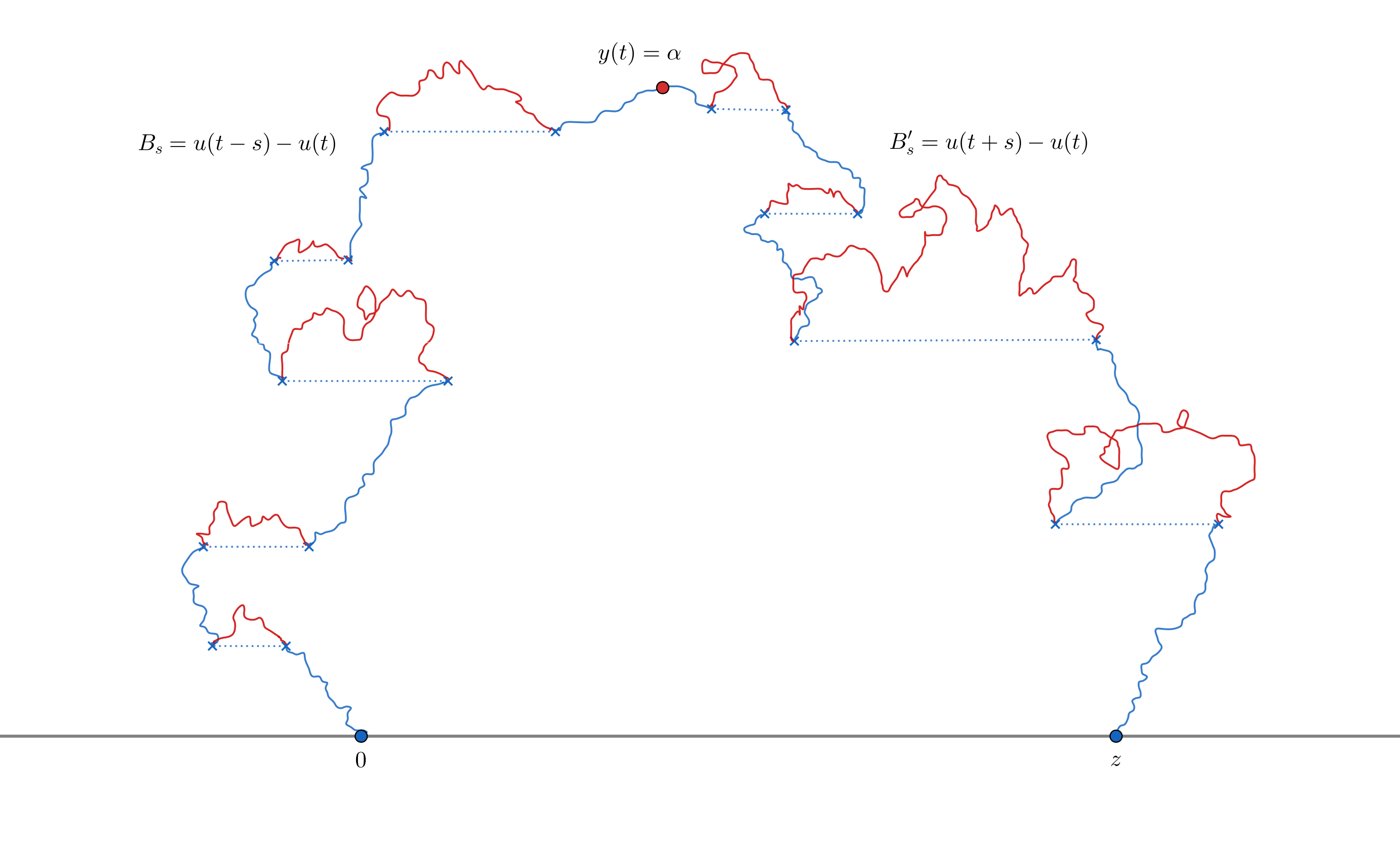
ut,←\displaystyle u^{t,\leftarrow} :=(u⁡(t−s)−u⁡(t))0≤s≤t,\displaystyle:=\left(u(t-s)-u(t)\right)_{0\leq s\leq t}, (2)
ut,→\displaystyle u^{t,\rightarrow} :=(u⁡(t+s)−u⁡(t))0≤s≤R⁡(u)−t.\displaystyle:=\left(u(t+s)-u(t)\right)_{0\leq s\leq R(u)-t}. (3)

If we set for a∈[0,y⁡(t)]a\in[0,y(t)],

Tat,←\displaystyle T_{a}^{t,\leftarrow} :=inf{s≥0,y⁡(t−s)=a},\displaystyle:=\inf\left\{s\geq 0,\;y(t-s)=a\right\}, (4)
Tat,→\displaystyle T_{a}^{t,\rightarrow} :=inf{s≥0,y⁡(t+s)=a},\displaystyle:=\inf\left\{s\geq 0,\;y(t+s)=a\right\}, (5)

we can write F(t)​(a)=ut,→​(Tat,→)−ut,←​(Tat,←)F^{(t)}(a)=u^{t,\rightarrow}(T_{a}^{t,\rightarrow})-u^{t,\leftarrow}(T_{a}^{t,\leftarrow}).

Lemma 2.5.

For any u∈U+u\in U^{+}, for all 0≤t≤R⁡(u)0\leq t\leq R(u), the function F(t)F^{(t)} is càdlàg.

Proof. Fix t∈[0,R⁡(u)]t\in[0,R(u)]. We want to show that F(t)F^{(t)} is càdlàg on [0,y⁡(t)][0,y(t)]. By usual properties of inverse of continuous functions (see Lemma 4.8 and the remark following it in Chapter 0 of Revuz-Yor [17]), a↦Tat,←a\mapsto T_{a}^{t,\leftarrow} and a↦Tat,→a\mapsto T_{a}^{t,\rightarrow} are càdlàg (in aa). Hence F(t)F^{(t)} is càdlàg since uu is continuous. ∎

2.4 Bismut’s description of Itô’s measure in ℍ\mathbb{H}

In the case of one-dimensional Itô’s measure n+n_{+}, Bismut’s description roughly states that if we pick an excursion uu at random according to n+n_{+}, and some time 0≤t≤R⁡(u)0\leq t\leq R(u) according to the Lebesgue measure, then the "law" of u⁡(t)u(t) is the Lebesgue measure and conditionally on u⁡(t)=αu(t)=\alpha, the left and right parts of uu (seen from u⁡(t)u(t)) are independent Brownian motions killed at −α-\alpha (see Theorem 4.7, Chap. XII in [17]). We deduce an analogous result in the case of Itô’s measure in ℍ\mathbb{H} and we apply it to show that for 𝔫+−\mathfrak{n}_{+}-almost every excursion, there is no loop remaining above any horizontal level.

Proposition 2.6.

(Bismut’s description of Itô’s measure in ℍ\mathbb{H})

Let 𝔫¯+\overline{\mathfrak{n}}_{+} be the measure defined on ℝ+×U+\mathbb{R}_{+}\times U^{+} by

𝔫¯+(dt,du)=𝟙{0≤t≤R(u)}dt𝔫+(du).\overline{\mathfrak{n}}_{+}(\mathrm{d}t,\mathrm{d}u)=\mathds{1}_{\{0\leq t\leq R(u)\}}\mathrm{d}t\,\mathfrak{n}_{+}(\mathrm{d}u).

Then under 𝔫¯+\overline{\mathfrak{n}}_{+} the "law" of (t,(x,y))↦y⁡(t)(t,(x,y))\mapsto y(t) is the Lebesgue measure d​α\mathrm{d}\alpha and conditionally on y⁡(t)=αy(t)=\alpha, ut,←=(u⁡(t−s)−u⁡(t))0≤s≤tu^{t,\leftarrow}=\left(u(t-s)-u(t)\right)_{0\leq s\leq t} and ut,→=(u⁡(t+s)−u⁡(t))0≤s≤R⁡(u)−tu^{t,\rightarrow}=\left(u(t+s)-u(t)\right)_{0\leq s\leq R(u)-t} are independent Brownian motions killed when reaching {ℑ(z)=−α}\left\{\Im(z)=-\alpha\right\}.

See Figure 3. Proposition 2.6 is a direct consequence of the one-dimensional analogous result, for which we refer to [17] (see Theorem 4.7, Chapter XII).

The next proposition ensures that for almost every excursion under 𝔫+\mathfrak{n}_{+}, there is no loop growing above any horizontal level. Let

ℒ:={u∈U+,∃0≤t≤R(u),∃0≤a<y(t),Δea(t)(u)=0},\mathscr{L}:=\{u\in U^{+},\;\exists 0\leq t\leq R(u),\;\exists 0\leq a<y(t),\;\Delta e_{a}^{(t)}(u)=0\},

be the set of excursions uu having a loop remaining above some level aa. Then we have :

Proposition 2.7.
𝔫+​(ℒ)=0.\mathfrak{n}_{+}\left(\mathscr{L}\right)=0.

Proof. We first prove the result under 𝔫¯+\overline{\mathfrak{n}}_{+}, namely

𝔫¯+({(t,u)∈ℝ+×U+,∃0≤a<y(t),Δea(t)(u)=0})=0.\overline{\mathfrak{n}}_{+}\left(\{(t,u)\in\mathbb{R}_{+}\times U^{+},\;\;\exists 0\leq a<y(t),\;\Delta e_{a}^{(t)}(u)=0\}\right)=0.

Recall the notation (2)-(5). From Bismut’s description of 𝔫¯+\overline{\mathfrak{n}}_{+} we get

𝔫¯+({(t,u)∈ℝ+×U+,∃0≤a<y(t),Δea(t)(u)=0})\displaystyle\overline{\mathfrak{n}}_{+}\left(\{(t,u)\in\mathbb{R}_{+}\times U^{+},\;\;\exists 0\leq a<y(t),\;\Delta e_{a}^{(t)}(u)=0\}\right)
=𝔫¯+({(t,u)∈ℝ+×U+,∃0≤a<y(t),ut,→(Tat,→)=ut,←(Tat,←)})\displaystyle=\overline{\mathfrak{n}}_{+}\left(\{(t,u)\in\mathbb{R}_{+}\times U^{+},\;\;\exists 0\leq a<y(t),\;u^{t,\rightarrow}(T_{a}^{t,\rightarrow})=u^{t,\leftarrow}(T_{a}^{t,\leftarrow})\}\right)
=∫0∞dαℙ(∃0<a≤α,XTa=XTa′′),\displaystyle=\int_{0}^{\infty}\mathrm{d}\alpha\,\mathbb{P}\left(\exists 0<a\leq\alpha,\,X_{T_{a}}=X^{\prime}_{T^{\prime}_{a}}\right),

where XX and X′X^{\prime} are independent linear Brownian motions, and TaT_{a} and Ta′T^{\prime}_{a} are hitting times of aa of other independent Brownian motions (corresponding to the imaginary parts). Now, XTaX_{T_{a}} and XTa′′X^{\prime}_{T^{\prime}_{a}} are independent symmetric Cauchy processes, and therefore XTa−XTa′′X_{T_{a}}-X^{\prime}_{T^{\prime}_{a}} is again a Cauchy process (see Section 4, Chap. III of [17]). Since points are polar for the symmetric Cauchy process (see [3], Chap. II, Section 5), we obtain ℙ(∃0<a≤α,XTa=XTa′′)=0\mathbb{P}\left(\exists 0<a\leq\alpha,\,X_{T_{a}}=X^{\prime}_{T^{\prime}_{a}}\right)=0 and under 𝔫¯+\overline{\mathfrak{n}}_{+} the result is proved.

Refer to caption
Figure 3: Bismut’s description of 𝔫+\mathfrak{n}_{+}

To extend the result to 𝔫+\mathfrak{n}_{+}, we notice that if u∈ℒu\in\mathscr{L}, then the set of tt’s satisfying the definition of ℒ\mathscr{L} has positive Lebesgue measure: namely, it contains all the times until the loop comes back to itself. This translates into

ℒ⊂{u∈U+,∫0R⁡(u)𝟙{∃0≤a<y(t),Δea(t)(u)=0}dt>0}.\mathscr{L}\subset\left\{u\in U^{+},\,\int_{0}^{R(u)}\mathds{1}_{\{\exists 0\leq a<y(t),\;\Delta e_{a}^{(t)}(u)=0\}}\mathrm{d}t>0\right\}.

But

𝔫+(∫0R⁡(u)𝟙{∃0≤a<y(t),Δea(t)(u)=0}dt)\displaystyle\mathfrak{n}_{+}\left(\int_{0}^{R(u)}\mathds{1}_{\{\exists 0\leq a<y(t),\;\Delta e_{a}^{(t)}(u)=0\}}\mathrm{d}t\right)
=∫U+∫0R⁡(u)𝟙{∃0≤a<y(t),Δea(t)(u)=0}dt𝔫+(du)\displaystyle=\int_{U^{+}}\int_{0}^{R(u)}\mathds{1}_{\{\exists 0\leq a<y(t),\;\Delta e_{a}^{(t)}(u)=0\}}\mathrm{d}t\,\mathfrak{n}_{+}(\mathrm{d}u)
=𝔫¯+({(t,u)∈ℝ+×U+,∃0≤a<y(t),Δea(t)(u)=0}).\displaystyle=\overline{\mathfrak{n}}_{+}\left(\{(t,u)\in\mathbb{R}_{+}\times U^{+},\;\;\exists 0\leq a<y(t),\;\Delta e_{a}^{(t)}(u)=0\}\right).

Hence, by the first step of the proof,

𝔫+(∫0R⁡(u)𝟙{∃0≤a<y(t),Δea(t)(u)=0}dt)=0,\mathfrak{n}_{+}\left(\int_{0}^{R(u)}\mathds{1}_{\{\exists 0\leq a<y(t),\;\Delta e_{a}^{(t)}(u)=0\}}\mathrm{d}t\right)=0,

which gives ∫0R⁡(u)𝟙{∃0≤a<y(t),Δea(t)(u)=0}dt=0\displaystyle\int_{0}^{R(u)}\mathds{1}_{\{\exists 0\leq a<y(t),\;\Delta e_{a}^{(t)}(u)=0\}}\mathrm{d}t=0 for 𝔫+−\mathfrak{n}_{+}-almost every excursion, and the desired result. ∎

2.5 The locally largest excursion

In [6], the authors give a canonical way to construct the growth-fragmentation, through the so-called locally largest fragment. We want to mimic this construction in our case.

In order to define the locally largest excursion, we set for u∈U+u\in U^{+} and 0≤t≤R⁡(u)0\leq t\leq R(u),

S(t):=sup{a∈[0,y(t)],∀ 0≤a′≤a,|F(t)(a′)|≥|F(t)(a′⁣−)−F(t)(a′)|}.S(t):=\sup\left\{a\in[0,y(t)],\quad\forall\,0\leq a^{\prime}\leq a,\;\big|F^{(t)}(a^{\prime})\big|\geq\big|F^{(t)}(a^{\prime-})-F^{(t)}(a^{\prime})\big|\right\}.

Observe that the supremum is taken over a non-empty set by Lemma 2.5 as soon as y⁡(t)>0y(t)>0 and u⁡(R⁡(u))≠0u(R(u))\neq 0. Let

S:=sup0≤t≤R⁡(u)​S​(t).S:=\underset{0\leq t\leq R(u)}{\sup}S(t).

In the case of Brownian excursions, the following proposition holds.

Proposition 2.8.

For almost every uu under 𝔫+\mathfrak{n}_{+}, there exists a unique 0≤t∙≤R⁡(u)0\leq t^{\bullet}\leq R(u) such that S⁡(t∙)=SS(t^{\bullet})=S. Moreover, S=ℑ⁡(z∙)S=\Im(z^{\bullet}) where z∙=u⁡(t∙)z^{\bullet}=u(t^{\bullet}).

We call (ea(t∙))0≤a≤ℑ⁡(z∙)\left(e_{a}^{(t^{\bullet})}\right)_{0\leq a\leq\Im(z^{\bullet})} the locally largest excursion and (Ξ⁡(a)=Δ​ea(t∙))0≤a≤ℑ⁡(z∙)\left(\Xi(a)=\Delta e_{a}^{(t^{\bullet})}\right)_{0\leq a\leq\Im(z^{\bullet})} the locally largest fragment.

Thus Ξ\Xi is the length of the excursion which is locally the largest, meaning that at any level aa where the locally largest excursion splits, Ξ\Xi is larger (in absolute value) than the length of the other excursion. See Figure 4 for a picture of z∙z^{\bullet}. Following [6], we will see it as the Eve particle of our growth-fragmentation process.

Refer to caption
Figure 4: The locally largest excursion.

Proof. Existence. We deal with the excursions uu satisfying the following properties, which happen 𝔫+\mathfrak{n}_{+}-almost everywhere : uu has no loop above any horizontal level (see Proposition 2.7) and yy has distinct local minima. Take a convergent sequence (tn,n≥1)(t_{n},n\geq 1) such that S⁡(tn)S(t_{n}) converges to SS, and denote by t∙t^{\bullet} the limit of tnt_{n}. We have necessarily, by definition of S⁡(t)S(t), that y⁡(tn)≥S⁡(tn)y(t_{n})\geq S(t_{n}). By continuity of yy, we get that y⁡(t∙)≥Sy(t^{\bullet})\geq S. Take a<Sa<S. For nn large enough, since a<y⁡(t∙)a<y(t^{\bullet}), we observe that tnt_{n} and t∙t^{\bullet} are in the same excursion above aa, i.e. ea(t∙)=ea(tn)e_{a}^{(t^{\bullet})}=e_{a}^{(t_{n})}. For such nn, F(tn)​(a′)=F(t∙)​(a′)F^{(t_{n})}(a^{\prime})=F^{(t^{\bullet})}(a^{\prime}) for all a′≤aa^{\prime}\leq a. Moreover, for nn large enough, S⁡(tn)>aS(t_{n})>a hence for all a′≤aa^{\prime}\leq a, |F(t∙)​(a′)|=|F(tn)​(a′)|≥|F(tn)​(a′⁣−)−F(tn)​(a′)|=|F(t∙)​(a′⁣−)−F(t∙)​(a′)|\big|F^{(t^{\bullet})}(a^{\prime})\big|=\big|F^{(t_{n})}(a^{\prime})\big|\geq\big|F^{(t_{n})}(a^{\prime-})-F^{(t_{n})}(a^{\prime})\big|=\big|F^{(t^{\bullet})}(a^{\prime-})-F^{(t^{\bullet})}(a^{\prime})\big|. It implies that S⁡(t∙)≥aS(t^{\bullet})\geq a, hence S⁡(t∙)≥SS(t^{\bullet})\geq S by taking aa arbitrarily close to SS. We found t∙t^{\bullet} such that S⁡(t∙)=SS(t^{\bullet})=S.

We show that y⁡(t∙)=Sy(t^{\bullet})=S. Notice that, for all 0≤t≤R⁡(u)0\leq t\leq R(u), by right-continuity of F(t)F^{(t)}, the set

A(t):={0≤a≤y(t),∀ 0≤a′≤a,|F(t)(a′)|≥|F(t)(a′⁣−)−F(t)(a′)|}A(t):=\left\{0\leq a\leq y(t),\quad\forall\,0\leq a^{\prime}\leq a,\;\big|F^{(t)}(a^{\prime})\big|\geq\big|F^{(t)}(a^{\prime-})-F^{(t)}(a^{\prime})\big|\right\}

is open in [0,y⁡(t)][0,y(t)]. Indeed, for a<y⁡(t)a<y(t), ea(t)e_{a}^{(t)} cannot be an excursion with size 00 by assumption, and so by right-continuity, we can take δ>0\delta>0 such that on [a,a+δ][a,a+\delta], F(t)F^{(t)} takes values in (34​F(t)​(a),32​F(t)​(a))\left(\frac{3}{4}F^{(t)}(a),\frac{3}{2}F^{(t)}(a)\right) (in the case F(t)​(a)>0F^{(t)}(a)>0, without loss of generality). For such a δ\delta, and for any a′∈[a,a+δ]a^{\prime}\in[a,a+\delta], F(t)​(a′)>34​F(t)​(a)>34​23​F(t)​(a′⁣−)=12​F(t)​(a′⁣−)F^{(t)}(a^{\prime})>\frac{3}{4}F^{(t)}(a)>\frac{3}{4}\frac{2}{3}F^{(t)}(a^{\prime-})=\frac{1}{2}F^{(t)}(a^{\prime-}), and F(t)​(a′⁣−)≥0F^{(t)}(a^{\prime-})\geq 0. These two inequalities imply that |F(t)​(a′)|≥|F(t)​(a′⁣−)−F(t)​(a′)||F^{(t)}(a^{\prime})|\geq|F^{(t)}(a^{\prime-})-F^{(t)}(a^{\prime})|.

Now suppose that S<y⁡(t∙)S<y(t^{\bullet}) and let us find a contradiction. We have A⁡(t∙)=[0,S)A(t^{\bullet})=[0,S), hence |F(t∙)​(S)|<|F(t∙)​(S−)−F(t∙)​(S)||F^{(t^{\bullet})}(S)|<|F^{(t^{\bullet})}(S^{-})-F^{(t^{\bullet})}(S)|. Write ea(t∙)=uIe_{a}^{(t^{\bullet})}=u_{I} with I=(ia,−,ia,+)I=(i_{a,-},i_{a,+}), so that F(t∙)​(a)=x⁡(ia,+)−x⁡(ia,−)F^{(t^{\bullet})}(a)=x(i_{a,+})-x(i_{a,-}). Since F(t∙)F^{(t^{\bullet})} jumps at SS, either i⋅,−i_{\cdot,-} or i⋅,+i_{\cdot,+} jumps at SS. Both cases cannot happen at the same time because local minima of yy are all distinct. Suppose for example that iS−,−<iS,−i_{S^{-},-}<i_{S,-}. Take t∈(iS−,−,iS,−)t\in(i_{S^{-},-},i_{S,-}) (see Figure 5). We have F(t)​(a)=F(t∙)​(a)F^{(t)}(a)=F^{(t^{\bullet})}(a) for all a<Sa<S and

F(t)​(S)\displaystyle F^{(t)}(S) =x⁡(iS,−)−x⁡(iS−,−)=x⁡(iS−,+)−x⁡(iS−,−)−(x⁡(iS,+)−x⁡(iS,−))\displaystyle=x(i_{S,-})-x(i_{S^{-},-})=x(i_{S^{-},+})-x(i_{S^{-},-})-(x(i_{S,+})-x(i_{S,-}))
=F(t∙)​(S−)−F(t∙)​(S)\displaystyle=F^{(t^{\bullet})}(S^{-})-F^{(t^{\bullet})}(S)
=F(t)​(S−)−F(t∙)​(S).\displaystyle=F^{(t)}(S^{-})-F^{(t^{\bullet})}(S).
Refer to caption
Figure 5: Construction of the locally largest excursion.

We deduce that |F(t)​(S)|=|F(t∙)​(S−)−F(t∙)​(S)|>|F(t∙)​(S)|=|F(t)​(S−)−F(t)​(S)||F^{(t)}(S)|=|F^{(t^{\bullet})}(S^{-})-F^{(t^{\bullet})}(S)|>|F^{(t^{\bullet})}(S)|=|F^{(t)}(S^{-})-F^{(t)}(S)|. Then A⁡(t)A(t) is open in [0,y⁡(t)][0,y(t)], contains SS, and we have y⁡(t)>Sy(t)>S. Hence supA⁡(t)>S\sup A(t)>S which gives the desired contradiction.

Uniqueness. Suppose that S⁡(t)=S⁡(t′)=SS(t)=S(t^{\prime})=S with t<t′t<t^{\prime} and let us find again a contradiction. We showed that necessarily, y⁡(t)=y⁡(t′)=Sy(t)=y(t^{\prime})=S. Let tm∈[t,t′]t_{m}\in[t,t^{\prime}] such that y⁡(tm)=min⁡{y⁡(r),r∈[t,t′]}y(t_{m})=\min\left\{y(r),\,r\in[t,t^{\prime}]\right\}. Set am:=y⁡(tm)a_{m}:=y(t_{m}). Observe that tt and t′t^{\prime} cannot be starting times or ending times of an excursion of yy (otherwise we could have extended the locally largest fragment inside this excursion for some positive height). Hence am<Sa_{m}<S. At level ama_{m}, there must be a splitting into two excursions (one straddling time tt, the other t′t^{\prime}) with equal size. It happens on a negligible set under 𝔫+\mathfrak{n}_{+}. To see it, we can restrict to t<t′t<t^{\prime} rationals and use the Markov property at time t′t^{\prime}. ∎

2.6 Disintegration of Itô’s measure over the size of the excursions

We are interested in conditioning Itô’s measure of excursions in ℍ\mathbb{H} on their initial size, i.e. in fixing the value of x⁡(R⁡(u))=zx(R(u))=z. This will allow us to define probability measures γz\gamma_{z} which disintegrate 𝔫+\mathfrak{n}_{+} over the value of the endpoint zz. Properties will simply transfer from 𝔫+\mathfrak{n}_{+} to γz\gamma_{z} via the disintegration formula. Define Pra→bP_{r}^{a\rightarrow b} as the law of the one-dimensional Brownian bridge of length rr between aa and bb, and Πr\Pi_{r} as the law of a three-dimensional Bessel (B​E​S3BES^{3}) bridge of length rr from 00 to 00.

Proposition 2.9.

We have the following disintegration formula

𝔫+=∫ℝd​z2​π​z2​γz,\mathfrak{n}_{+}=\int_{\mathbb{R}}\frac{\mathrm{d}z}{2\pi z^{2}}\,\gamma_{z}, (6)

where for z≠0z\neq 0,

γz=∫ℝ+d​v​e−1/2v2​v2​Pv​z20→z⊗Πv​z2.\gamma_{z}=\int_{\mathbb{R}_{+}}\mathrm{d}v\,\frac{e^{-1/2v}}{2v^{2}}\,P_{vz^{2}}^{0\rightarrow z}\otimes\Pi_{vz^{2}}. (7)

Proof. Let ff and gg be two nonnegative measurable functions defined on 𝒳\mathscr{X} and 𝒳0\mathscr{X}_{0} respectively. Thanks to Itô’s description of n+n_{+} (see [17], Chap. XII, Theorem 4.2), we have

∫Uf⁡(x)​g​(y)​𝔫+​(𝑑x,𝑑y)\displaystyle\int_{U}f(x)g(y)\,\mathfrak{n}_{+}(\mathrm{d}x,\mathrm{d}y) =∫Uf⁡(x)​g​(y)​n+​(𝑑y)​ℙ​(XR⁡(y)∈𝑑x)\displaystyle=\int_{U}f(x)g(y)\,n_{+}(\mathrm{d}y)\mathbb{P}\left(X^{R(y)}\in\mathrm{d}x\right)
=∫ℝ+d​r2​2​π​r3​∫𝒳f⁡(x)​Πr​[g]​ℙ​(Xr∈𝑑x).\displaystyle=\int_{\mathbb{R}_{+}}\frac{\mathrm{d}r}{2\sqrt{2\pi r^{3}}}\int_{\mathscr{X}}f(x)\,\Pi_{r}[g]\,\mathbb{P}\left(X^{r}\in\mathrm{d}x\right).

Now, decomposing on the value of the Gaussian r.v. XrX_{r} yields

∫Uf⁡(x)​g​(y)​𝔫+​(𝑑x,𝑑y)=∫ℝ+d​r2​2​π​r3​∫ℝd​z​e−z2/2r2​π​r​Πr​[g]​Er0→z​[f].\int_{U}f(x)g(y)\,\mathfrak{n}_{+}(\mathrm{d}x,\mathrm{d}y)=\int_{\mathbb{R}_{+}}\frac{\mathrm{d}r}{2\sqrt{2\pi r^{3}}}\int_{\mathbb{R}}\mathrm{d}z\frac{e^{-z^{2}/2r}}{\sqrt{2\pi r}}\Pi_{r}[g]\,E_{r}^{0\rightarrow z}\left[f\right].

We finally perform the change of variables v⁡(r)=r/z2v(r)=r/z^{2} to get

∫Uf⁡(x)​g​(y)​𝔫+​(𝑑x,𝑑y)=∫ℝd​z2​π​z2​∫ℝ+d​v​e−1/2v2​v2​Ev​z20→z​[f]​Πv​z2​[g].\int_{U}f(x)g(y)\,\mathfrak{n}_{+}(\mathrm{d}x,\mathrm{d}y)=\int_{\mathbb{R}}\frac{\mathrm{d}z}{2\pi z^{2}}\int_{\mathbb{R}_{+}}\mathrm{d}v\,\frac{e^{-1/2v}}{2v^{2}}E_{vz^{2}}^{0\rightarrow z}\left[f\right]\,\Pi_{vz^{2}}[g].

∎

Lemma 2.10.

Let zz be a nonzero real number. The image measure of γz\gamma_{z} by the function which sends (x,y)(x,y) to

(x⁡(t​z2)z,y⁡(t​z2)|z|),0≤t≤R⁡(u)z2,\left(\frac{x(tz^{2})}{z},\frac{y(tz^{2})}{|z|}\right),\quad 0\leq t\leq\frac{R(u)}{z^{2}},

is γ1\gamma_{1}.

Proof. It comes from the definition of γz\gamma_{z} and the scaling property of B​E​S3BES^{3} bridge and Brownian bridge. ∎

2.7 The metric space of excursions in ℍ\mathbb{H}

Very often, results under γz\gamma_{z} can be obtained by proving the analog under the Itô’s measure 𝔫+\mathfrak{n}_{+}, and then disintegrating over z=x⁡(R⁡(u))z=x(R(u)). This usually provides results under γz\gamma_{z} for Lebesgue-almost every z>0z>0, and so we would like to study the continuity of z↦γzz\mapsto\gamma_{z}. This requires to define a topology on the space of excursions U+U^{+}. All these results will be stated for z>0z>0 because the scaling depends on the sign of the endpoint (Lemma 2.10), but they all extend to the general case.

We therefore introduce the usual distance

d⁡(u,v)=|R⁡(u)−R⁡(v)|+supt≥0|u⁡(t∧R⁡(u))−v⁡(t∧R⁡(v))|,d(u,v)=|R(u)-R(v)|+\sup_{t\geq 0}|u(t\wedge R(u))-v(t\wedge R(v))|,

where we identified δ\delta with the excursion with lifetime 00. The distance dd makes U+U^{+} into a Polish space. The following lemmas may come in useful.

Lemma 2.11.

The map Δ:u∈U+↦Δ​u=x⁡(R⁡(u))\Delta:u\in U^{+}\mapsto\Delta u=x(R(u)) is continuous.

Proof. This is straightforward since |x⁡(R⁡(u))−x′​(R⁡(u′))|=|u⁡(R⁡(u))−u′​(R⁡(u′))|≤d⁡(u,u′)|x(R(u))-x^{\prime}(R(u^{\prime}))|=|u(R(u))-u^{\prime}(R(u^{\prime}))|\leq d(u,u^{\prime}) for u=(x,y)u=(x,y) and u′=(x′,y′)u^{\prime}=(x^{\prime},y^{\prime}). ∎

Lemma 2.12.

Let u∈U+u\in U^{+}. Then z∈ℝ+∗↦u(z):=zu(⋅/z2)=(zu(t/z2),0≤t≤R(u)z2)z\in\mathbb{R}^{*}_{+}\mapsto u^{(z)}:=zu(\cdot/z^{2})=\left(zu(t/z^{2}),0\leq t\leq R(u)z^{2}\right) is a continuous function.

Proof. Let z0>0z_{0}>0. Then for all z>0z>0

d⁡(u(z),u(z0))=R⁡(u)​|z2−z02|+supt≥0|z​u​(tz2∧R⁡(u))−z0​u​(tz02∧R⁡(u))|.d(u^{(z)},u^{(z_{0})})=R(u)|z^{2}-z_{0}^{2}|+\sup_{t\geq 0}\left|zu\left(\frac{t}{z^{2}}\wedge R(u)\right)-z_{0}u\left(\frac{t}{z_{0}^{2}}\wedge R(u)\right)\right|.

The second term is

supt≥0|z​u​(tz2∧R⁡(u))−z0​u​(tz02∧R⁡(u))|\displaystyle\sup_{t\geq 0}\left|zu\left(\frac{t}{z^{2}}\wedge R(u)\right)-z_{0}u\left(\frac{t}{z_{0}^{2}}\wedge R(u)\right)\right|
≤z​supt≥0|u⁡(tz2∧R⁡(u))−u⁡(tz02∧R⁡(u))|+supt≥0|(z−z0)​u​(tz2∧R⁡(u))|\displaystyle\leq z\sup_{t\geq 0}\left|u\left(\frac{t}{z^{2}}\wedge R(u)\right)-u\left(\frac{t}{z_{0}^{2}}\wedge R(u)\right)\right|+\sup_{t\geq 0}\left|(z-z_{0})u\left(\frac{t}{z^{2}}\wedge R(u)\right)\right|
≤z​supt≥0|u⁡(tz2∧R⁡(u))−u⁡(tz02∧R⁡(u))|+|z−z0|​supt≥0|u⁡(t)|.\displaystyle\leq z\sup_{t\geq 0}\left|u\left(\frac{t}{z^{2}}\wedge R(u)\right)-u\left(\frac{t}{z_{0}^{2}}\wedge R(u)\right)\right|+|z-z_{0}|\sup_{t\geq 0}|u(t)|.

We conclude by using the uniform continuity of uu. ∎

If we equip the set 𝒫⁡(U+)\mathcal{P}(U^{+}) of probability measures on U+U^{+} with the topology of weak convergence, we have the following result.

Proposition 2.13.

The map z∈ℝ+∗↦γzz\in\mathbb{R}_{+}^{*}\mapsto\gamma_{z} is continuous.

Proof. Let GG be a continuous bounded function on U+U^{+}. Then by scaling (Lemma 2.10), for all z>0z>0,

γz​(G)=γ1​[G⁡(u(z))].\gamma_{z}(G)=\gamma_{1}\left[G(u^{(z)})\right].

Applying Lemma 2.12 together with the dominated convergence theorem yields the desired result. ∎

Also, we will use the continuity of the excursions cut at horizontal levels. Recall from Section 2.3 that ℐ⁡(a){\mathcal{I}}(a) is the set of times when the excursion u∈U+u\in U^{+} lies above aa, and for each connected component II of ℐ⁡(a){\mathcal{I}}(a), uIu_{I} denotes the associated excursion above aa. The path uIu_{I} is an excursion above aa, II is the time interval of uIu_{I}, and the size or length of uIu_{I} is the difference between its endpoint and its starting point.

On {Ta<∞}\{T_{a}<\infty\}, we rank the excursions above aa according to the absolute value of their size. Write z1a,+=z1a,+(u),z2a,+=z2a,+(u),…z^{a,+}_{1}=z^{a,+}_{1}(u),z^{a,+}_{2}=z^{a,+}_{2}(u),\ldots for the sizes, ranked in descending order of their absolute value, and e1a,+=e1a,+(u),e2a,+=e2a,+(u),…e^{a,+}_{1}=e^{a,+}_{1}(u),e^{a,+}_{2}=e^{a,+}_{2}(u),\ldots for the corresponding excursions. This is possible since for any fixed ε>0\varepsilon>0 there are only finitely many excursions with length larger than ε\varepsilon in absolute value.

Proposition 2.14.

Let a>0a>0 and z>0z>0. For any i≥1i\geq 1, the function eia,+e^{a,+}_{i} is continuous on U+U^{+} on the event {Ta<∞}\{T_{a}<\infty\} outside a γz\gamma_{z}-negligible set.

Proof. We consider the set ℰ\mathscr{E} of trajectories u=(x,y)u=(x,y) such that Ta<∞T_{a}<\infty and satisfying the following conditions, which occur with γz\gamma_{z}-probability one when conditioned on touching aa: the level aa is not a local minimum for yy, there exist infinitely many excursions above aa, all excursions touch aa only at their starting point and endpoint, the sizes (zia,+,i≥1)(z_{i}^{a,+},\,i\geq 1) of the excursions are all distinct. Let i≥1i\geq 1 and u=(x,y)∈ℰu=(x,y)\in\mathscr{E}. We want to show that ei(a,+)e_{i}^{(a,+)} is continuous at uu.

Let tt be a time in the excursion eia,+e_{i}^{a,+}, i.e. such that y⁡(t)>ay(t)>a and ea(t)=eia,+e^{(t)}_{a}=e_{i}^{a,+}. We restrict our attention to u′=(x′,y′)∈ℰu^{\prime}=(x^{\prime},y^{\prime})\in\mathscr{E} close enough to uu so that y′​(t)>ay^{\prime}(t)>a and we will write ea′(t)e_{a}^{\prime(t)} for the excursion of u′u^{\prime} corresponding to tt. Let ε>0\varepsilon>0.

  • •

    First, we want to find δ>0\delta>0 such that, whenever d⁡(u,u′)<δd(u,u^{\prime})<\delta, the durations of the excursions ea(t)e_{a}^{(t)} and ea′(t)e_{a}^{\prime(t)} are close, namely |R⁡(ea′(t))−R⁡(ea(t))|<ε|R(e_{a}^{\prime(t)})-R(e^{(t)}_{a})|<\varepsilon. Write (i−​(a),i+​(a))(i_{-}(a),i_{+}(a)), and (i−′​(a),i+′​(a))(i^{\prime}_{-}(a),i^{\prime}_{+}(a)), for the excursion time intervals corresponding to ea(t)e_{a}^{(t)} and ea′(t)e_{a}^{\prime(t)} respectively. For simplicity, we take the notation R=R⁡(ea(t))R=R(e^{(t)}_{a}) and R′=R⁡(ea′(t))R^{\prime}=R(e^{\prime(t)}_{a}). Since aa is not a local minimum for yy, there exist times t1∈(i−​(a)−ε2,i−​(a))t_{1}\in(i_{-}(a)-\frac{\varepsilon}{2},i_{-}(a)) and t2∈(i+​(a),i+​(a)+ε2)t_{2}\in(i_{+}(a),i_{+}(a)+\frac{\varepsilon}{2}) when yy is strictly below aa. Take δ1∈(0,a)\delta_{1}\in(0,a) such that y⁡(t1)y(t_{1}) and y⁡(t2)y(t_{2}) are in (0,a−δ1)(0,a-\delta_{1}). Let u′=(x′,y′)∈ℰu^{\prime}=(x^{\prime},y^{\prime})\in\mathscr{E} such that d⁡(u,u′)<δ12d(u,u^{\prime})<\frac{\delta_{1}}{2}. We deduce that y′​(t1)<y⁡(t1)+δ12<ay^{\prime}(t_{1})<y(t_{1})+\frac{\delta_{1}}{2}<a and similarly y′​(t2)<ay^{\prime}(t_{2})<a. This implies that i−′​(a)≥t1>i−​(a)−ε2i^{\prime}_{-}(a)\geq t_{1}>i_{-}(a)-\frac{\varepsilon}{2} and i+′​(a)≤t2<i+​(a)+ε2i^{\prime}_{+}(a)\leq t_{2}<i_{+}(a)+\frac{\varepsilon}{2}. Likewise, pick two times t3∈(i−​(a),i−​(a)+ε2)t_{3}\in(i_{-}(a),i_{-}(a)+{\varepsilon\over 2}) and t4∈(i+​(a)−ε2,i+​(a))t_{4}\in(i_{+}(a)-\frac{\varepsilon}{2},i_{+}(a)) such that t3<t<t4t_{3}<t<t_{4}. Since the excursion ea(t)e_{a}^{(t)} touches level aa only at its extremities, the distance between the compact u⁡([t3,t4])u([t_{3},t_{4}]) and the closed set {ℑ(z)=a}\{\Im(z)=a\} is positive, and so, on the interval [t3,t4][t_{3},t_{4}], yy remains above, say, a+δ2a+\delta_{2} where δ2>0\delta_{2}>0. Then when d⁡(u,u′)<δ22d(u,u^{\prime})<\frac{\delta_{2}}{2}, the excursion ea′(t)e_{a}^{\prime(t)} will satisfy i−′​(a)<t3<i−​(a)+ε2i^{\prime}_{-}(a)<t_{3}<i_{-}(a)+\frac{\varepsilon}{2} and i+′​(a)>t4>i+​(a)−ε2i^{\prime}_{+}(a)>t_{4}>i_{+}(a)-\frac{\varepsilon}{2}. Therefore, when d⁡(u,u′)<δ=min⁡(δ12,δ22)d(u,u^{\prime})<\delta=\min(\frac{\delta_{1}}{2},\frac{\delta_{2}}{2}), we get that |i−′​(a)−i−​(a)|<ε2|i^{\prime}_{-}(a)-i_{-}(a)|<\frac{\varepsilon}{2} and |i+′​(a)−i+​(a)|<ε2|i^{\prime}_{+}(a)-i_{+}(a)|<\frac{\varepsilon}{2}, so in particular |R′−R|<ε|R^{\prime}-R|<\varepsilon. Observe that we not only proved that the durations are close, but also that the times i−,i−′i_{-},i^{\prime}_{-} (and i+,i+′i_{+},i^{\prime}_{+}) are close, and this will be useful in the remainder of the proof.

  • •

    Secondly, we show that we can take δ′>0\delta^{\prime}>0 small enough so that

    sups≥0|ea(t)​(s∧R)−ea′(t)​(s∧R′)|<ε,\sup_{s\geq 0}|e_{a}^{(t)}(s\wedge R)-e_{a}^{\prime(t)}(s\wedge R^{\prime})|<\varepsilon,

    whenever d⁡(u,u′)<δ′d(u,u^{\prime})<\delta^{\prime}.

    Take η=η⁡(ε)>0\eta=\eta(\varepsilon)>0 some modulus of uniform continuity of uu with respect to ε\varepsilon. The previous paragraph gives the existence of δ>0\delta>0 such that when u′∈ℰu^{\prime}\in\mathscr{E} and d⁡(u,u′)<δd(u,u^{\prime})<\delta, |i−′​(a)−i−​(a)|<η/3|i^{\prime}_{-}(a)-i_{-}(a)|<\eta/3 and |i+′​(a)−i+​(a)|<η/3|i^{\prime}_{+}(a)-i_{+}(a)|<\eta/3. Without loss of generality, we can assume that δ<ε\delta<\varepsilon. Define δ′=min⁡(δ,η)\delta^{\prime}=\min(\delta,\eta), and let u′∈ℰu^{\prime}\in\mathscr{E} such that d⁡(u,u′)<δ′d(u,u^{\prime})<\delta^{\prime}. For all s≥0s\geq 0, we have

    |ea(t)​(s∧R)−ea′(t)​(s∧R′)|\displaystyle|e_{a}^{(t)}(s\wedge R)-e_{a}^{\prime(t)}(s\wedge R^{\prime})|
    =|u⁡(i−​(a)+(s∧R))−u⁡(i−​(a))−u′​(i−′​(a)+(s∧R′))+u′​(i−′​(a))|\displaystyle=\left|u(i_{-}(a)+(s\wedge R))-u(i_{-}(a))-u^{\prime}(i^{\prime}_{-}(a)+(s\wedge R^{\prime}))+u^{\prime}(i^{\prime}_{-}(a))\right|
    ≤|u⁡(i−​(a))−u′​(i−′​(a))|+|u⁡(i−​(a)+(s∧R))−u⁡(i−′​(a)+(s∧R′))|.\displaystyle\leq\left|u(i_{-}(a))-u^{\prime}(i^{\prime}_{-}(a))\right|+\left|u(i_{-}(a)+(s\wedge R))-u(i^{\prime}_{-}(a)+(s\wedge R^{\prime}))\right|. (8)

    Now,

    |u⁡(i−​(a))−u′​(i−′​(a))|≤|u⁡(i−​(a))−u⁡(i−′​(a))|+|u⁡(i−′​(a))−u′​(i−′​(a))|,\left|u(i_{-}(a))-u^{\prime}(i^{\prime}_{-}(a))\right|\leq\left|u(i_{-}(a))-u(i^{\prime}_{-}(a))\right|+\left|u(i^{\prime}_{-}(a))-u^{\prime}(i^{\prime}_{-}(a))\right|,

    and so by uniform continuity of uu and because d⁡(u,u′)<δ′<εd(u,u^{\prime})<\delta^{\prime}<\varepsilon, we obtain

    |u⁡(i−​(a))−u′​(i−′​(a))|≤2​ε.\left|u(i_{-}(a))-u^{\prime}(i^{\prime}_{-}(a))\right|\leq 2\varepsilon. (9)

    Similarly, the second term of (8) is

    |u⁡(i−​(a)+(s∧R))−u′​(i−′​(a)+(s∧R′))|\displaystyle\left|u(i_{-}(a)+(s\wedge R))-u^{\prime}(i^{\prime}_{-}(a)+(s\wedge R^{\prime}))\right|
    ≤|u⁡(i−​(a)+(s∧R))−u⁡(i−′​(a)+(s∧R′))|\displaystyle\leq\left|u(i_{-}(a)+(s\wedge R))-u(i^{\prime}_{-}(a)+(s\wedge R^{\prime}))\right|
    +|u⁡(i−′​(a)+(s∧R′))−u′​(i−′​(a)+(s∧R′))|,\displaystyle\quad+\left|u(i^{\prime}_{-}(a)+(s\wedge R^{\prime}))-u^{\prime}(i^{\prime}_{-}(a)+(s\wedge R^{\prime}))\right|,

    and since |i−​(a)+(s∧R)−i−′​(a)−(s∧R′)|<η|i_{-}(a)+(s\wedge R)-i^{\prime}_{-}(a)-(s\wedge R^{\prime})|<\eta, we can conclude in the same way that

    |u⁡(i−​(a)+(s∧R))−u′​(i−′​(a)+(s∧R′))|≤2​ε.\left|u(i_{-}(a)+(s\wedge R))-u^{\prime}(i^{\prime}_{-}(a)+(s\wedge R^{\prime}))\right|\leq 2\varepsilon. (10)

    Inequalities (8), (9) and (10) give

    |ea(t)​(s∧R)−ea′(t)​(s∧R′)|≤4​ε,|e_{a}^{(t)}(s\wedge R)-e_{a}^{\prime(t)}(s\wedge R^{\prime})|\leq 4\varepsilon,

    which is the desired result.

So far, we proved that ea(t)e_{a}^{(t)} is continuous at uu. To conclude, we need an argument to say that this is the ii-th excursion above aa for u′u^{\prime} sufficiently close to uu.

  • •

    Finally, we show that we can take δ′′>0\delta^{\prime\prime}>0 small enough so that ei′a,+=ea′(t)e_{i}^{\prime a,+}=e_{a}^{\prime(t)} whenever d⁡(u,u′)<δ′′d(u,u^{\prime})<\delta^{\prime\prime}.

    This is derived in two steps.

    • -

      Step 1: Let η>0\eta>0, and introduce, for u′∈ℰu^{\prime}\in\mathscr{E}, the number Nη​(u′)N_{\eta}(u^{\prime}) of time intervals (i−,i+)(i_{-},i_{+}) of excursions of u′u^{\prime} above aa such that i+−i−>ηi_{+}-i_{-}>\eta. Note that Nη​(u′)≤R⁡(u′)η<∞N_{\eta}(u^{\prime})\leq\frac{R(u^{\prime})}{\eta}<\infty. We take η\eta such that uu has no excursion time interval above aa satisfying i+−i−=ηi_{+}-i_{-}=\eta. The first step consists in proving that for u′∈ℰu^{\prime}\in\mathscr{E} sufficiently close to uu, Nη​(u′)=Nη​(u)N_{\eta}(u^{\prime})=N_{\eta}(u). From the first point (applied Nη​(u)N_{\eta}(u) times), we know that for δ>0\delta>0 small enough, Nη​(u′)≥Nη​(u)N_{\eta}(u^{\prime})\geq N_{\eta}(u) whenever d⁡(u,u′)<δd(u,u^{\prime})<\delta. To prove that Nη​(u′)≤Nη​(u)N_{\eta}(u^{\prime})\leq N_{\eta}(u) holds as well when δ\delta is sufficiently small, we use an argument by contradiction and we consider a sequence (un)n≥1(u_{n})_{n\geq 1} of elements in ℰ\mathscr{E} such that d⁡(u,un)→0d(u,u_{n})\rightarrow 0 and Nη​(un)≥Nη​(u)+1N_{\eta}(u_{n})\geq N_{\eta}(u)+1. Consider Nη​(u)+1N_{\eta}(u)+1 distinct excursion time intervals (ij,−(n),ij,+(n))(i^{(n)}_{j,-},i^{(n)}_{j,+}), 1≤j≤Nη​(u)+11\leq j\leq N_{\eta}(u)+1, of unu_{n} above aa such that ij,+(n)−ij,−(n)>ηi^{(n)}_{j,+}-i^{(n)}_{j,-}>\eta. We can write the corresponding excursions ea(tj(n))​(un)e_{a}^{(t^{(n)}_{j})}(u_{n}) for some tj(n)t_{j}^{(n)}’s. Moreover, we may take tj(n)t_{j}^{(n)} such that |ij,+(n)−tj(n)|>η/2|i^{(n)}_{j,+}-t_{j}^{(n)}|>\eta/2 and |ij,−(n)−tj(n)|>η/2|i^{(n)}_{j,-}-t_{j}^{(n)}|>\eta/2. Since |R⁡(u)−R⁡(un)|→0|R(u)-R(u_{n})|\rightarrow 0, we can assume (up to some extraction) that when nn goes to infinity, ij,+(n)→ij,+i^{(n)}_{j,+}\rightarrow i_{j,+}, ij,−(n)→ij,−i^{(n)}_{j,-}\rightarrow i_{j,-} and tj(n)→tj∈[0,R⁡(u)]t_{j}^{(n)}\rightarrow t_{j}\in[0,R(u)], for some ij,+,ij,−,tj∈[0,R⁡(u)]i_{j,+},i_{j,-},t_{j}\in[0,R(u)]. From un→uu_{n}\rightarrow u, we deduce that for all jj, y⁡(ij,−)=ay(i_{j,-})=a and y⁡(ij,+)=ay(i_{j,+})=a. For nn large enough, because ij,+(n)−ij,−(n)>ηi^{(n)}_{j,+}-i^{(n)}_{j,-}>\eta and |ij,±(n)−tj(n)|>η/2|i^{(n)}_{j,\pm}-t_{j}^{(n)}|>\eta/2, we have ea(tj(n))​(un)=ea(tj)​(un)e_{a}^{(t_{j}^{(n)})}(u_{n})=e_{a}^{(t_{j})}(u_{n}). Now consider ea(tj)​(u)e_{a}^{(t_{j})}(u). From the two previous points, ea(tj)​(un)→ea(tj)​(u)e_{a}^{(t_{j})}(u_{n})\rightarrow e_{a}^{(t_{j})}(u). For any time s∈(i−,i+)s\in(i_{-},i_{+}), we have y⁡(s)>ay(s)>a (otherwise aa would be a local minimum of yy). Hence (ij,−,ij,+)(i_{j,-},i_{j,+}) is an excursion time interval for uu and ij,+−ij,−>ηi_{j,+}-i_{j,-}>\eta. Therefore we constructed Nη​(u)+1N_{\eta}(u)+1 distinct excursion time intervals above aa for uu, which gives the desired contradiction.

    • -

      Step 2: Suppose for example that zia,+>0z_{i}^{a,+}>0. Take δ<zia,+6\delta<\frac{z_{i}^{a,+}}{6} and η=η⁡(δ)>0\eta=\eta(\delta)>0 some modulus of uniform continuity for uu with respect to δ\delta. We can assume in order to apply Step 1 that η\eta is such that uu has no excursion above aa satisfying |i+−i−|=η|i_{+}-i_{-}|=\eta. We look at the N:=Nη​(u)N:=N_{\eta}(u) excursions e1,…,eNe_{1},\ldots,e_{N} of uu above aa (ranked by decreasing order of the absolute value of their sizes) such that |i+−i−|>η|i_{+}-i_{-}|>\eta, and denote their sizes by z1,…,zNz_{1},\ldots,z_{N}. Observe that the first ii excursions among these are the excursions e1a,+,…,eia,+e_{1}^{a,+},\ldots,e_{i}^{a,+}. Indeed, if |i+−i−|≤η|i_{+}-i_{-}|\leq\eta, then by uniform continuity,

      |u⁡(i+)−u⁡(i−)|≤δ<zia,+.|u(i_{+})-u(i_{-})|\leq\delta<z_{i}^{a,+}.

      Let ε′=12​(min1≤k≤N−1⁡|zk+1−zk|∧zi)\varepsilon^{\prime}=\frac{1}{2}\left(\min_{1\leq k\leq N-1}|z_{k+1}-z_{k}|\wedge z_{i}\right) (this is positive since all the sizes are assumed to be distinct in ℰ\mathscr{E}). Take times t1,…,tNt_{1},\ldots,t_{N} in the excursion time intervals of e1,…,eNe_{1},\ldots,e_{N}. Thanks to Step 1 and the first point of the proof (applied NN times), there exists δ′>0\delta^{\prime}>0 such that for d⁡(u,u′)<δ′d(u,u^{\prime})<\delta^{\prime}, if we denote by (i−′(tk),i+′(tk))(i_{-}^{\prime(t_{k})},i_{+}^{\prime(t_{k})}) the excursion time interval of ea′(tk),1≤k≤Ne^{\prime(t_{k})}_{a},1\leq k\leq N, then

      1. (i)

        Nη​(u′)=NN_{\eta}(u^{\prime})=N,

      2. (ii)

        the excursions ea′(tk),1≤k≤N,e^{\prime(t_{k})}_{a},1\leq k\leq N, are distinct,

      3. (iii)

        ∀ 1≤k≤N,|i+′(tk)−i−′(tk)|>η\forall\,1\leq k\leq N,\quad|i_{+}^{\prime(t_{k})}-i_{-}^{\prime(t_{k})}|>\eta,

      4. (iv)

        ∀ 1≤k≤N,|zka,+−Δ​ea′(tk)|≤ε′.\forall\,1\leq k\leq N,\quad|z^{a,+}_{k}-\Delta e^{\prime(t_{k})}_{a}|\leq\varepsilon^{\prime}.

      An easy calculation shows that by our choice of ε′\varepsilon^{\prime} and (iv), the Δ​ea′(tk),1≤k≤N\Delta e^{\prime(t_{k})}_{a},1\leq k\leq N, are ranked in decreasing order, and that

      ∀ 1≤k≤i,Δ​ea′(tk)>zia,+2.\forall\,1\leq k\leq i,\quad\Delta e^{\prime(t_{k})}_{a}>\frac{z_{i}^{a,+}}{2}. (11)

      In addition, by (i), (ii) and (iii), the ea′(tk),1≤k≤N,e^{\prime(t_{k})}_{a},1\leq k\leq N, are the excursions of u′u^{\prime} above aa satisfying |i+−i−|>η|i_{+}-i_{-}|>\eta.

      Now set δ′′=min⁡(δ,δ′)\delta^{\prime\prime}=\min(\delta,\delta^{\prime}) and assume that d⁡(u,u′)<δ′′d(u,u^{\prime})<\delta^{\prime\prime}. Then for all 1≤k≤i1\leq k\leq i, ea′(tk)=eka,+​(u′)e^{\prime(t_{k})}_{a}=e_{k}^{a,+}(u^{\prime}). Indeed, if (i−,i+)(i_{-},i_{+}) is an excursion time interval of u′u^{\prime} such that |i+−i−|≤η|i_{+}-i_{-}|\leq\eta, then

      |u′​(i+)−u′​(i−)|≤|u′​(i+)−u⁡(i+)|+|u⁡(i+)−u⁡(i−)|+|u⁡(i−)−u′​(i−)|≤3​δ,|u^{\prime}(i_{+})-u^{\prime}(i_{-})|\leq|u^{\prime}(i_{+})-u(i_{+})|+|u(i_{+})-u(i_{-})|+|u(i_{-})-u^{\prime}(i_{-})|\leq 3\delta,

      and so in particular |u′​(i+)−u′​(i−)|<zia,+2|u^{\prime}(i_{+})-u^{\prime}(i_{-})|<\frac{z_{i}^{a,+}}{2}. This proves that the first ii excursions of u′u^{\prime} are among the NN previous excursions satisfying |i+−i−|>η|i_{+}-i_{-}|>\eta. Since these are ranked in decreasing order, necessarily ea′(tk)=eka,+​(u′)e^{\prime(t_{k})}_{a}=e_{k}^{a,+}(u^{\prime}) for all 1≤k≤i1\leq k\leq i, which concludes the proof.

Putting these three points together, we proved that eia,+e_{i}^{a,+} is continuous on ℰ\mathscr{E} which has full probability under γz\gamma_{z}, hence Proposition 2.14. ∎

3 Markovian properties

In this section, we are interested in Markovian properties of excursions cut at horizontal levels. Time will therefore be indexed by the height aa of the cutting.

3.1 The branching property for excursions in ℍ\mathbb{H}

Consider an excursion under the measure γz\gamma_{z}. Then cutting it at some height a>0a>0 yields a family of excursions above aa as defined in Section 2.3. Our aim is to show that conditionally on what happens below aa, these are independent and distributed according to the measures γz\gamma_{z}, where zz is the size of the corresponding excursion. We shall first consider the case when the original excursion is taken under the Itô’s measure 𝔫+\mathfrak{n}_{+} in ℍ\mathbb{H}, and then transfer the property to γz\gamma_{z} by the previous disintegration result (6).

Let 𝒢a0\mathcal{G}^{0}_{a} be the σ\sigma–field containing all the information of the trajectory below level aa and 𝒢a\mathcal{G}_{a} be the completion of 𝒢a0\mathcal{G}^{0}_{a} with the 𝔫+\mathfrak{n}_{+}–negligible sets. In other words, the σ\sigma–field 𝒢a0\mathcal{G}^{0}_{a} is generated by the trajectory uu once you cut out the excursions above aa, and close up the time gaps. A formal definition of this process is the process uu indexed by the generalized inverse of t↦∫0t𝟙{u(s)≤a}dst\mapsto\int_{0}^{t}\mathds{1}_{\{u(s)\leq a\}}\mathrm{d}s.

Refer to caption
Figure 6: The excursion process above aa.

Recall from Section 2.7 that z1a,+,z2a,+,…z^{a,+}_{1},z^{a,+}_{2},\ldots are the sizes of the excursions above aa, ranked in decreasing order of their absolute value, and e1a,+,e2a,+,…e^{a,+}_{1},e^{a,+}_{2},\ldots are the corresponding excursions.

Proposition 3.1.

(Branching property for excursions in ℍ\mathbb{H} under 𝔫+\mathfrak{n}_{+})

For any A∈𝒢aA\in\mathcal{G}_{a}, and for all nonnegative measurable functions G1,…,Gk:U+→ℝ+G_{1},\ldots,G_{k}:U^{+}\rightarrow\mathbb{R}_{+}, k≥1k\geq 1,

𝔫+(𝟙{Ta<∞}𝟙A∏i=1kGi(eia,+))=𝔫+(𝟙{Ta<∞}𝟙A∏i=1kγzia,+[Gi]).\mathfrak{n}_{+}\left(\mathds{1}_{\{T_{a}<\infty\}}\mathds{1}_{A}\prod_{i=1}^{k}G_{i}(e^{a,+}_{i})\right)=\mathfrak{n}_{+}\left(\mathds{1}_{\{T_{a}<\infty\}}\mathds{1}_{A}\prod_{i=1}^{k}\gamma_{z^{a,+}_{i}}[G_{i}]\right). (12)

Proof. Lemma 2.4 ensures that on the event {Ta<∞}\{T_{a}<\infty\}, the trajectory uu after time TaT_{a} has the law of a killed Brownian motion. Excursion theory tells us that given the excursions below aa, the excursions above aa form a Poisson point process on U+U^{+} with intensity L​𝔫+​(d​u)L\,\mathfrak{n}_{+}({\rm d}u), where LL is the total local time at level aa, see Figure 6. Finally, conditionally on the sizes (zia,+)i≥1(z_{i}^{a,+})_{i\geq 1} of the excursions above aa, these excursions are independent with law γzia,+\gamma_{z_{i}^{a,+}}. We deduce the proposition since the σ\sigma-field 𝒢a\mathcal{G}_{a} is generated by ℱTa\mathcal{F}_{T_{a}}, the excursions below aa, and the sizes (zia,+)i≥1(z_{i}^{a,+})_{i\geq 1}. ∎

We can now transfer this property to the probability measures γz\gamma_{z}.

Proposition 3.2.

(Branching property for excursions in ℍ\mathbb{H} under γz\gamma_{z})

Let z∈ℝ∖{0}z\in\mathbb{R}\setminus\{0\}. For any A∈𝒢aA\in\mathcal{G}_{a}, and for all nonnegative measurable functions G1,…,Gk:U+→ℝ+G_{1},\ldots,G_{k}:U^{+}\rightarrow\mathbb{R}_{+}, k≥1k\geq 1,

γz(𝟙{Ta<∞}𝟙A∏i=1kGi(eia,+))=γz(𝟙{Ta<∞}𝟙A∏i=1kγzia,+[Gi]).\gamma_{z}\left(\mathds{1}_{\{T_{a}<\infty\}}\mathds{1}_{A}\prod_{i=1}^{k}G_{i}(e^{a,+}_{i})\right)=\gamma_{z}\left(\mathds{1}_{\{T_{a}<\infty\}}\mathds{1}_{A}\prod_{i=1}^{k}\gamma_{z^{a,+}_{i}}[G_{i}]\right).

Proof. It suffices to prove the proposition for bounded continuous functions G1,…,Gk:U+→ℝ+G_{1},\ldots,G_{k}:U^{+}\rightarrow\mathbb{R}_{+}, k≥1k\geq 1. Take a nonnegative measurable function f:ℝ→ℝ+f:\mathbb{R}\rightarrow\mathbb{R}_{+} and a bounded continuous function h:U+→ℝ+h:U^{+}\rightarrow\mathbb{R}_{+} which is 𝒢a−\mathcal{G}_{a}-measurable. Observe that x⁡(R⁡(u))x(R(u)) is 𝒢a−\mathcal{G}_{a}-measurable as a function of uu. From Proposition 3.1, we know that

𝔫+(𝟙{Ta<∞}h(u)f(x(R(u)))∏i=1kGi(eia,+))=𝔫+(𝟙{Ta<∞}h(u)f(x(R(u)))∏i=1kγzia,+[Gi]).\mathfrak{n}_{+}\left(\mathds{1}_{\{T_{a}<\infty\}}h(u)f(x(R(u)))\prod_{i=1}^{k}G_{i}(e^{a,+}_{i})\right)=\mathfrak{n}_{+}\left(\mathds{1}_{\{T_{a}<\infty\}}h(u)f(x(R(u)))\prod_{i=1}^{k}\gamma_{z^{a,+}_{i}}[G_{i}]\right).

Thanks to the disintegration formula (6), we can split 𝔫+\mathfrak{n}_{+} over the size:

∫ℝd​z2​π​z2f(z)γz(𝟙{Ta<∞}h∏i=1kGi(eia,+))=∫ℝd​z2​π​z2f(z)γz(𝟙{Ta<∞}h∏i=1kγzia,+[Gi]).\int_{\mathbb{R}}\frac{\mathrm{d}z}{2\pi z^{2}}\,f(z)\,\gamma_{z}\left(\mathds{1}_{\{T_{a}<\infty\}}h\prod_{i=1}^{k}G_{i}(e^{a,+}_{i})\right)=\int_{\mathbb{R}}\frac{\mathrm{d}z}{2\pi z^{2}}\,f(z)\,\gamma_{z}\left(\mathds{1}_{\{T_{a}<\infty\}}h\prod_{i=1}^{k}\gamma_{z^{a,+}_{i}}[G_{i}]\right).

Since this holds for any ff, it entails for Lebesgue-almost every z∈ℝz\in\mathbb{R},

γz(𝟙{Ta<∞}h∏i=1kGi(eia,+))=γz(𝟙{Ta<∞}h∏i=1kγzia,+[Gi]).\gamma_{z}\left(\mathds{1}_{\{T_{a}<\infty\}}h\prod_{i=1}^{k}G_{i}(e^{a,+}_{i})\right)=\gamma_{z}\left(\mathds{1}_{\{T_{a}<\infty\}}h\prod_{i=1}^{k}\gamma_{z^{a,+}_{i}}[G_{i}]\right). (13)

To prove that this holds for all zz, we need a continuity argument. We first treat the case z=1z=1. Using the scaling property 2.10 of the measures γz\gamma_{z}, for z>0z>0 the left-hand side of (13) is

γ1(𝟙{Ta/z<∞}h(u(z))∏i=1kGi(eia,+(u(z))))\gamma_{1}\left(\mathds{1}_{\{T_{a/z}<\infty\}}h(u^{(z)})\prod_{i=1}^{k}G_{i}(e^{a,+}_{i}(u^{(z)}))\right)

where we recall from Lemma 2.12 that u(z)=zu(⋅/z2)u^{(z)}=zu(\cdot/z^{2}). The right-hand side term, on the other hand, is

γz(𝟙{Ta<∞}h∏i=1kγzia,+[Gi])=γ1(𝟙{Ta/z<∞}h(u(z))∏i=1kγzia,+​(u(z))[Gi]),\gamma_{z}\left(\mathds{1}_{\{T_{a}<\infty\}}h\prod_{i=1}^{k}\gamma_{z^{a,+}_{i}}[G_{i}]\right)=\gamma_{1}\left(\mathds{1}_{\{T_{a/z}<\infty\}}h(u^{(z)})\prod_{i=1}^{k}\gamma_{z^{a,+}_{i}(u^{(z)})}[G_{i}]\right),

and so (13) translates into

γ1(𝟙{Ta/z<∞}h(u(z))∏i=1kGi(eia,+(u(z))))=γ1(𝟙{Ta/z<∞}h(u(z))∏i=1kγzia,+​(u(z))[Gi]),\gamma_{1}\left(\mathds{1}_{\{T_{a/z}<\infty\}}h(u^{(z)})\prod_{i=1}^{k}G_{i}(e^{a,+}_{i}(u^{(z)}))\right)=\gamma_{1}\left(\mathds{1}_{\{T_{a/z}<\infty\}}h(u^{(z)})\prod_{i=1}^{k}\gamma_{z^{a,+}_{i}(u^{(z)})}[G_{i}]\right), (14)

for Lebesgue-almost every z>0z>0. In particular this is true for a dense set of zz. Taking z↘1z\searrow 1 along some decreasing sequence, we first get that u(z)→uu^{(z)}\rightarrow u by Lemma 2.12 and Ta/z→TaT_{a/z}\rightarrow T_{a} by left-continuity of the stopping times. In addition, for all 1≤i≤k1\leq i\leq k, zia,+​(u(z))→zia,+​(u)z^{a,+}_{i}(u^{(z)})\rightarrow z^{a,+}_{i}(u) γ1\gamma_{1}-almost surely because z→zia,+​(u(z))=Δ​eia,+​(u(z))z\rightarrow z^{a,+}_{i}(u^{(z)})=\Delta e_{i}^{a,+}(u^{(z)}) is a continuous function (outside a negligible set) by Lemmas 2.11, 2.12 and Proposition 2.14. Finally, by continuity of z↦γzz\mapsto\gamma_{z} (Lemma 2.13), for all 1≤i≤k1\leq i\leq k, γzia,+​(u(z))​[Gi]→γzia,+​[Gi]\gamma_{z^{a,+}_{i}(u^{(z)})}[G_{i}]\rightarrow\gamma_{z^{a,+}_{i}}[G_{i}]. Applying the dominated convergence theorem to both sides of equation (14) triggers

γ1(𝟙{Ta<∞}h∏i=1kGi(eia,+))=γ1(𝟙{Ta<∞}h∏i=1kγzia,+[Gi]).\gamma_{1}\left(\mathds{1}_{\{T_{a}<\infty\}}h\prod_{i=1}^{k}G_{i}(e^{a,+}_{i})\right)=\gamma_{1}\left(\mathds{1}_{\{T_{a}<\infty\}}h\prod_{i=1}^{k}\gamma_{z^{a,+}_{i}}[G_{i}]\right).

and concludes the proof of Proposition 3.2 for z=1z=1. The general case follows by scaling. ∎

3.2 The locally largest evolution

Recall that Proposition 2.8 gives a canonical choice of excursion at level a>0a>0, which is the locally largest excursion ea(t∙)e_{a}^{(t^{\bullet})}. One may wonder whether the locally largest fragment Ξ⁡(a)=Δ​ea(t∙)\Xi(a)=\Delta e_{a}^{(t^{\bullet})} still exhibits some kind of Markovian behavior. The following theorem answers this question.

Theorem 3.3.

Let z>0z>0. Under γz\gamma_{z}, (Ξ⁡(a))0≤a<ℑ⁡(z∙)(\Xi(a))_{0\leq a<\Im(z^{\bullet})} is distributed as the positive self-similar Markov process (Za)0≤a<ζ(Z_{a})_{0\leq a<\zeta} with index 11 starting from zz whose Lamperti representation is

Za=z​exp⁡(ξ⁡(τ⁡(z−1​a))),Z_{a}=z\exp(\xi(\tau(z^{-1}a))),

where ξ\xi is the Lévy process with Laplace exponent Ψ⁡(q):=ln⁡γz​[eq​ξ​(1)]\Psi(q):=\ln\gamma_{z}[\mathrm{e}^{q\xi(1)}] given by

Ψ⁡(q)=−4π​q+2π​∫y>−ln⁡(2)(eq​y−1−q⁡(ey−1))​e−y​d​y(ey−1)2,q<3,\Psi(q)=-\frac{4}{\pi}q+\frac{2}{\pi}\int_{y>-\ln(2)}\left(\mathrm{e}^{qy}-1-q(\mathrm{e}^{y}-1)\right)\frac{\mathrm{e}^{-y}\mathrm{d}y}{(\mathrm{e}^{y}-1)^{2}},\quad q<3, (15)

τ\tau is the time change

τ(a)=inf{s≥0,∫0seξ⁡(u)du>a},\tau(a)=\inf\left\{s\geq 0,\;\int_{0}^{s}\mathrm{e}^{\xi(u)}\mathrm{d}u>a\right\},

and ζ=inf{a≥0,Za=0}\zeta=\inf\{a\geq 0,\;Z_{a}=0\}.

Recall the notation (2)-(5). We set

uat,⇌:=((ut,←(s+Tat,←))s≥0,(ut,→(s+Tat,→))s≥0)−(ut,←(Tat,←),ut,←(Tat,←)),u^{t,\rightleftharpoons}_{a}:=\left((u^{t,\leftarrow}(s+T_{a}^{t,\leftarrow}))_{s\geq 0},(u^{t,\rightarrow}(s+T_{a}^{t,\rightarrow}))_{s\geq 0}\right)-\left(u^{t,\leftarrow}(T_{a}^{t,\leftarrow}),u^{t,\leftarrow}(T_{a}^{t,\leftarrow})\right),

with the convention that ut,⇌au^{t,\rightleftharpoons}_{a} is a cemetery function if y⁡(t)<ay(t)<a.

We shall use the following lemma. Note that the lemma does not disintegrate the law of ut∙,⇌au^{t^{\bullet},\rightleftharpoons}_{a} on the measures γz\gamma_{z}, and one has to be careful not to confuse the zz appearing in the integral with the value of x⁡(R⁡(u))x(R(u)) (the reader should keep track of x⁡(R⁡(u))x(R(u)) in the proof).

Lemma 3.4.

Let (X,Y)(X,Y) and (X′,Y′)(X^{\prime},Y^{\prime}) be under ℙ\mathbb{P} two independent planar Brownian motions starting from the origin, and for b≤0b\leq 0, TbT_{b} and Tb′T^{\prime}_{b} their respective hitting times of {ℑ(z)=b}\{\Im(z)=b\}, with T~b\widetilde{T}_{b} and T~b′\widetilde{T}^{\prime}_{b} denoting the hitting times of {ℑ(z)<b}\{\Im(z)<b\}. For α≥a≥0\alpha\geq a\geq 0, and z∈ℝz\in\mathbb{R} we set

ℰα,a,z:={|z+(XTb′′−XTb)|≥|(XT~b′′−XT~b)−(XTb′′−XTb)|,∀b∈[−α,−α+a]}.\mathcal{E}_{\alpha,a,z}:=\left\{\left|z+(X^{\prime}_{T^{\prime}_{b}}-X_{T_{b}})\right|\geq\left|(X^{\prime}_{\widetilde{T}^{\prime}_{b}}-X_{\widetilde{T}_{b}})-(X^{\prime}_{T^{\prime}_{b}}-X_{T_{b}})\right|,\,\forall\,b\in[-\alpha,-\alpha+a]\right\}.

Then, for any nonnegative measurable function HH,

𝔫+[H(uat∙,⇌)𝟙{a<ℑ(z∙)}]=∫zd​z2​π​z2h(−a,z),\mathfrak{n}_{+}[H(u^{t^{\bullet},\rightleftharpoons}_{a})\mathds{1}_{\{a<\Im(z^{\bullet})\}}]=\int_{z}{\mathrm{d}z\over 2\pi z^{2}}h(-a,z),

where hh is :

h⁡(−a,z):=𝔼⁡[H⁡((Xs,Ys)s∈[0,T−a],(z+Xs′,Ys′)s∈[0,T−a′]),ℰa,a,z].h(-a,z):=\mathbb{E}\left[H\left((X_{s},Y_{s})_{s\in[0,T_{-a}]},(z+X^{\prime}_{s},Y^{\prime}_{s})_{s\in[0,T^{\prime}_{-a}]}\right),\,\mathcal{E}_{a,a,z}\right].

Remark. Observe that the process (Ξ⁡(a′),a′≤a)(\Xi(a^{\prime}),\,a^{\prime}\leq a) is measurable with respect to ut∙,⇌au^{t^{\bullet},\rightleftharpoons}_{a}. We denote by 𝔻\mathbb{D} the space of càdlàg real-valued paths with finite lifetime, endowed with the local Skorokhod topology. It results from the lemma that for any nonnegative measurable function on 𝔻\mathbb{D},

𝔫+[H(Ξ(b),b∈[0,a])𝟙{a<ℑ(z∙)}]=∫zd​z2​π​z2h(−a,z),\mathfrak{n}_{+}[H(\Xi(b),\,b\in[0,a])\mathds{1}_{\{a<\Im(z^{\bullet})\}}]=\int_{z}{\mathrm{d}z\over 2\pi z^{2}}h(-a,z),

where hh is now :

h⁡(−a,z):=𝔼⁡[H⁡(z+XT−a+b′′−XT−a+b,b∈[0,a]),ℰa,a,z].h(-a,z):=\mathbb{E}\left[H\left(z+X^{\prime}_{T^{\prime}_{-a+b}}-X_{T_{-a+b}},\,b\in[0,a]\right),\,\mathcal{E}_{a,a,z}\right].

Proof. Integrating over the duration of the excursion ea(t∙)e_{a}^{(t^{\bullet})}, we see that for 𝔫+−\mathfrak{n}_{+}-almost every u∈U+u\in U^{+},

H(uat∙,⇌)𝟙{a<ℑ(z∙)}=∫0R⁡(u)H(uat,⇌)𝟙{y⁡(t)>a,ea(t∙)=ea(t)}1R⁡(ea(t))dt.H(u^{t^{\bullet},\rightleftharpoons}_{a})\mathds{1}_{\{a<\Im(z^{\bullet})\}}=\int_{0}^{R(u)}H(u^{t,\rightleftharpoons}_{a})\mathds{1}_{\{y(t)>a,\,e_{a}^{(t^{\bullet})}=e_{a}^{(t)}\}}{1\over R(e_{a}^{(t)})}\mathrm{d}t.

With Bismut’s description of 𝔫+\mathfrak{n}_{+} (Proposition 2.6, cf. Figure 3), we get

𝔫+[H(uat∙,⇌)𝟙{a<ℑ(z∙)}]=∫α>adα𝔼[H⁡(((X¯,Y¯),(X′¯,Y′¯)))T−α+a′+T−α+a,ℰα,a,0],\mathfrak{n}_{+}[H(u^{t^{\bullet},\rightleftharpoons}_{a})\mathds{1}_{\{a<\Im(z^{\bullet})\}}]=\int_{\alpha>a}\mathrm{d}\alpha\,\mathbb{E}\left[\frac{H\left(\left((\overline{X},\overline{Y}),(\overline{X^{\prime}},\overline{Y^{\prime}})\right)\right)}{T^{\prime}_{-\alpha+a}+T_{-\alpha+a}},\,\mathcal{E}_{\alpha,a,0}\right],

where

(X¯,Y¯)\displaystyle(\overline{X},\overline{Y}) =((X,Y)​(s+T−α+a))s∈[0,T−α−T−α+a]−(X,Y)​(T−α+a),\displaystyle=((X,Y)(s+T_{-\alpha+a}))_{s\in[0,T_{-\alpha}-T_{-\alpha+a}]}-(X,Y)(T_{-\alpha+a}),
(X′¯,Y′¯)\displaystyle(\overline{X^{\prime}},\overline{Y^{\prime}}) =((X′,Y′)​(s+T−α+a′))s∈[0,T−α′−T−α+a′]−(X,Y)​(T−α+a),\displaystyle=((X^{\prime},Y^{\prime})(s+T^{\prime}_{-\alpha+a}))_{s\in[0,T^{\prime}_{-\alpha}-T^{\prime}_{-\alpha+a}]}-(X,Y)(T_{-\alpha+a}),

with the notation (X,Y)​(s)=(Xs,Ys)(X,Y)(s)=(X_{s},Y_{s}). By the strong Markov property at times T−α+aT_{-\alpha+a} and T−α+a′T^{\prime}_{-\alpha+a}, the former integral can be expressed as

∫α>ad​α​𝔼​[h⁡(−a,XT−α+a′′−XT−α+a)​1T−α+a′+T−α+a],\int_{\alpha>a}\mathrm{d}\alpha\,\mathbb{E}\left[h\left(-a,X^{\prime}_{T^{\prime}_{-\alpha+a}}-X_{T_{-\alpha+a}}\right)\frac{1}{T^{\prime}_{-\alpha+a}+T_{-\alpha+a}}\right],

for hh defined as

h⁡(−a,z):=𝔼⁡[H⁡((Xs,Ys)s∈[0,T−a],(z+Xs′,Ys′)s∈[0,T−a′]),ℰa,a,z].h(-a,z):=\mathbb{E}\left[H\left((X_{s},Y_{s})_{s\in[0,T_{-a}]},(z+X^{\prime}_{s},Y^{\prime}_{s})_{s\in[0,T^{\prime}_{-a}]}\right),\,\mathcal{E}_{a,a,z}\right].

See Figure 3. By a change of variables, the former integral is

∫α≥0d​α​𝔼​[h⁡(−a,XT−α′′−XT−α)​1T−α′+T−α].\int_{\alpha\geq 0}\mathrm{d}\alpha\,\mathbb{E}\left[h(-a,X^{\prime}_{T^{\prime}_{-\alpha}}-X_{T_{-\alpha}})\frac{1}{T^{\prime}_{-\alpha}+T_{-\alpha}}\right].

Therefore, we proved that

𝔫+[H(uat∙,⇌)𝟙{a<ℑ(z∙)}]=∫α≥0dα𝔼[h(−a,XT−α′′−XT−α)1T−α′+T−α].\mathfrak{n}_{+}[H(u^{t^{\bullet},\rightleftharpoons}_{a})\mathds{1}_{\{a<\Im(z^{\bullet})\}}]=\int_{\alpha\geq 0}\mathrm{d}\alpha\,\mathbb{E}\left[h(-a,X^{\prime}_{T^{\prime}_{-\alpha}}-X_{T_{-\alpha}})\frac{1}{T^{\prime}_{-\alpha}+T_{-\alpha}}\right].

On the other hand, using again Bismut’s decomposition of 𝔫+\mathfrak{n}_{+}, we see that (actually for any hh),

𝔫+​[h⁡(−a,x⁡(R⁡(u)))]\displaystyle\mathfrak{n}_{+}[h(-a,x(R(u)))] =𝔫+​(∫0R⁡(u)h⁡(−a,x⁡(R⁡(u))​1R⁡(u)​𝑑t)CLOSE\displaystyle=\mathfrak{n}_{+}\left(\int_{0}^{R(u)}h(-a,x(R(u)){1\over R(u)}\mathrm{d}t\right)
=∫α≥0d​α​𝔼​[h⁡(−a,XT−α′′−XT−α)​1T−α′+T−α].\displaystyle=\int_{\alpha\geq 0}\mathrm{d}\alpha\,\mathbb{E}\left[h\left(-a,X^{\prime}_{T^{\prime}_{-\alpha}}-X_{T_{-\alpha}}\right)\frac{1}{T^{\prime}_{-\alpha}+T_{-\alpha}}\right].

Comparing the last two equations, we proved that

𝔫+[H(uat∙,⇌)𝟙{a<ℑ(z∙)}]=𝔫+[h(−a,x(R(u)))]=∫zd​z2​π​z2h(−a,z),\mathfrak{n}_{+}[H(u^{t^{\bullet},\rightleftharpoons}_{a})\mathds{1}_{\{a<\Im(z^{\bullet})\}}]=\mathfrak{n}_{+}[h(-a,x(R(u)))]=\int_{z}{\mathrm{d}z\over 2\pi z^{2}}h(-a,z),

by Proposition 2.9. ∎

We now come to the proof of Theorem 3.3. We closely follow the strategy of Le Gall and Riera in [16].

Proof. Let HH be a nonnegative bounded continuous function on 𝔻\mathbb{D}. From the previous Lemma 3.4, or rather from the Remark following its statement, we know that

𝔫+[H(Ξ(b),b∈[0,a])𝟙{a<ℑ(z∙)}]=∫zd​z2​π​z2h(−a,z),\mathfrak{n}_{+}[H(\Xi(b),\,b\in[0,a])\mathds{1}_{\{a<\Im(z^{\bullet})\}}]=\int_{z}{\mathrm{d}z\over 2\pi z^{2}}h(-a,z),

where hh is:

h⁡(−a,z)=𝔼⁡[H⁡(z+XT−a+b′′−XT−a+b,b∈[0,a]),ℰa,a,z].h(-a,z)=\mathbb{E}\left[H\left(z+X^{\prime}_{T^{\prime}_{-a+b}}-X_{T_{-a+b}},\,b\in[0,a]\right),\,\mathcal{E}_{a,a,z}\right].

Notice that, in the notation of Lemma 3.4, b↦XT~−b′′−XT~−bb\mapsto X^{\prime}_{\widetilde{T}^{\prime}_{-b}}-X_{\widetilde{T}_{-b}} is a (càdlàg) symmetric Cauchy process of Laplace exponent ψ⁡(λ)=−2​|λ|\psi(\lambda)=-2|\lambda| (for example, use that it is a Lévy process and Proposition 3.11 of [17], Chap. III). Denote by ηb\eta_{b} the double of the Cauchy process which under PzP_{z}, starts from zz, and Δ​ηb\Delta\eta_{b} the jump at time bb. Write η^b=η(a−b)−\hat{\eta}_{b}=\eta_{(a-b)^{-}} for the time-reversal of η\eta, Δ​η^b\Delta\hat{\eta}_{b} being the jump of η^\hat{\eta} at time bb. Then by definition of hh,

h(−a,z)=Ez[H(η^b,b∈[0,a]) 1{∀b∈[0,a],|η^b|≥|Δη^b|}].h(-a,z)=E_{z}\left[H(\hat{\eta}_{b},\,b\in[0,a])\,\mathds{1}_{\{\forall\,b\in[0,a],\;|\hat{\eta}_{b}|\geq|\Delta\hat{\eta}_{b}|\}}\right].

Now we want to reverse time in the function hh. Conditioning on ηa\eta_{a},

h⁡(−a,z)\displaystyle h(-a,z)
=1π∫ℝ2​a​d​x(2​a)2+(x−z)2Ez[H(η^b,b∈[0,a]) 1{∀b∈[0,a],|η^b|≥|Δη^b|}|ηa=x].\displaystyle=\frac{1}{\pi}\int_{\mathbb{R}}{2a\mathrm{d}x\over(2a)^{2}+(x-z)^{2}}E_{z}[H(\hat{\eta}_{b},\,b\in[0,a])\,\mathds{1}_{\{\forall\,b\in[0,a],\;|\hat{\eta}_{b}|\geq|\Delta\hat{\eta}_{b}|\}}|\eta_{a}=x].

By Corollary 3, Chap. II of [3]:

Ez[H(η^b,b∈[0,a]) 1{∀b∈[0,a],|η^b|≥|Δη^b|}|ηa=x]\displaystyle E_{z}[H(\hat{\eta}_{b},\,b\in[0,a])\,\mathds{1}_{\{\forall\,b\in[0,a],\;|\hat{\eta}_{b}|\geq|\Delta\hat{\eta}_{b}|\}}|\eta_{a}=x]
=Ex[H(ηb,b∈[0,a]) 1{∀b∈[0,a],|ηb|≥|Δηb|}|ηa=z].\displaystyle=E_{x}[H(\eta_{b},\,b\in[0,a])\,\mathds{1}_{\{\forall\,b\in[0,a],\;|\eta_{b}|\geq|\Delta\eta_{b}|\}}|\eta_{a}=z].

Indeed, the Cauchy process η\eta is symmetric, hence is itself its dual. We obtain

∫ℝd​z2​π​z2​h​(−a,z)=\displaystyle\int_{\mathbb{R}}{\mathrm{d}z\over 2\pi z^{2}}h(-a,z)=
∫ℝd​z2​π​z21π∫ℝ2​a​d​x(2​a)2+(x−z)2Ex[H(ηb,b∈[0,a]) 1{∀b∈[0,a],|ηb|≥|Δηb|}|ηa=z].\displaystyle\int_{\mathbb{R}}{\mathrm{d}z\over 2\pi z^{2}}\frac{1}{\pi}\int_{\mathbb{R}}{2a\mathrm{d}x\over(2a)^{2}+(x-z)^{2}}E_{x}[H(\eta_{b},\,b\in[0,a])\,\mathds{1}_{\{\forall\,b\in[0,a],\;|\eta_{b}|\geq|\Delta\eta_{b}|\}}|\eta_{a}=z].

We can rewrite it as

∫ℝd​x2​π​x21π∫ℝ2​a​d​z(2​a)2+(x−z)2Ex[x2z2H(ηb,b∈[0,a]) 1{∀b∈[0,a],|ηb|≥|Δηb|}|ηa=z],\int_{\mathbb{R}}{\mathrm{d}x\over 2\pi x^{2}}\frac{1}{\pi}\int_{\mathbb{R}}{2a\mathrm{d}z\over(2a)^{2}+(x-z)^{2}}E_{x}\left[{x^{2}\over z^{2}}H(\eta_{b},\,b\in[0,a])\,\mathds{1}_{\{\forall\,b\in[0,a],\;|\eta_{b}|\geq|\Delta\eta_{b}|\}}\bigg|\eta_{a}=z\right],

which is

∫ℝd​x2​π​x2Ex[x2(ηa)2H(ηb,b∈[0,a]) 1{∀b∈[0,a],|ηb|≥|Δηb|}].\int_{\mathbb{R}}{\mathrm{d}x\over 2\pi x^{2}}E_{x}\left[{x^{2}\over(\eta_{a})^{2}}H(\eta_{b},\,b\in[0,a])\,\mathds{1}_{\{\forall\,b\in[0,a],\;|\eta_{b}|\geq|\Delta\eta_{b}|\}}\right].

Now this gives the law of Ξ\Xi under the disintegration measures γx\gamma_{x}. Indeed, take instead of HH some nonnegative measurable function ff of the initial size Ξ⁡(0)\Xi(0), multiplied by HH. Then using the above expression, we find that

𝔫+[f(Ξ(0))H(Ξ(b),b∈[0,a])𝟙{a<ℑ(z∙)}]\displaystyle\mathfrak{n}_{+}[f(\Xi(0))H(\Xi(b),\,b\in[0,a])\mathds{1}_{\{a<\Im(z^{\bullet})\}}]
=∫ℝd​x2​π​x2f(x)Ex[x2(ηa)2H(ηb,b∈[0,a]) 1{∀b∈[0,a],|ηb|≥|Δηb|}].\displaystyle=\int_{\mathbb{R}}{\mathrm{d}x\over 2\pi x^{2}}f(x)E_{x}\left[{x^{2}\over(\eta_{a})^{2}}H(\eta_{b},\,b\in[0,a])\,\mathds{1}_{\{\forall\,b\in[0,a],\;|\eta_{b}|\geq|\Delta\eta_{b}|\}}\right].

Hence for Lebesgue-almost every x∈ℝx\in\mathbb{R},

γx[H(Ξ(b),b∈[0,a])𝟙{a<ℑ(z∙)}]=Ex[x2(ηa)2H(ηb,b∈[0,a]) 1{∀b∈[0,a],|ηb|≥|Δηb|}],\gamma_{x}[H(\Xi(b),\,b\in[0,a])\mathds{1}_{\{a<\Im(z^{\bullet})\}}]=E_{x}\left[{x^{2}\over(\eta_{a})^{2}}H(\eta_{b},\,b\in[0,a])\,\mathds{1}_{\{\forall\,b\in[0,a],\;|\eta_{b}|\geq|\Delta\eta_{b}|\}}\right], (16)

and by continuity this must hold for all x∈ℝx\in\mathbb{R}. Indeed, by scaling, the left-hand side of equation (16) is

γx[H(Ξ(b),b∈[0,a])𝟙{a<ℑ(z∙)}]=γ1[H(xΞ(x−1b),b∈[0,a])𝟙{a<xℑ(z∙)}].\gamma_{x}[H(\Xi(b),\,b\in[0,a])\mathds{1}_{\{a<\Im(z^{\bullet})\}}]=\gamma_{1}[H(x\Xi(x^{-1}b),\,b\in[0,a])\mathds{1}_{\{a<x\Im(z^{\bullet})\}}].

The right-hand term can be put in the same form by using the scale invariance of the Cauchy process. Since (16) holds for almost every xx, it must hold on a dense set of x>0x>0, and we may take x↗1x\nearrow 1 along a sequence. By dominated convergence, we get

γ1[H(Ξ(b),b∈[0,a])𝟙{a<ℑ(z∙)}]=E1[1(ηa)2H(ηb,b∈[0,a]) 1{∀b∈[0,a],|ηb|≥|Δηb|}],\gamma_{1}[H(\Xi(b),\,b\in[0,a])\mathds{1}_{\{a<\Im(z^{\bullet})\}}]=E_{1}\left[{1\over(\eta_{a})^{2}}H(\eta_{b},\,b\in[0,a])\,\mathds{1}_{\{\forall\,b\in[0,a],\;|\eta_{b}|\geq|\Delta\eta_{b}|\}}\right],

and this proves that equation (16) holds for x=1x=1. The general case x∈ℝx\in\mathbb{R} follows by scaling.

Notice that, almost surely, on the event {∀b∈[0,a],|ηb|≥|Δηb|}\{\forall\,b\in[0,a],\;|\eta_{b}|\geq|\Delta\eta_{b}|\}, if η0>0\eta_{0}>0, then ηb\eta_{b} is positive for all b∈[0,a]b\in[0,a]. We know from [9] that a symmetric Cauchy process starting from x>0x>0 killed when entering the negative half-line can be written using its Lamperti representation as x​eξ0​(τ0​(a))x\mathrm{e}^{\xi^{0}(\tau^{0}(a))} where

τ0(a):=∫0ad​sηs=inf{s≥0,∫0sxeξ0​(u)du≥a},\tau^{0}(a):=\int_{0}^{a}\frac{\mathrm{d}s}{\eta_{s}}=\inf\left\{s\geq 0,\;\int_{0}^{s}x\mathrm{e}^{\xi^{0}(u)}\mathrm{d}u\geq a\right\},

and (ξ0​(a),a≥0)(\xi^{0}(a),\,a\geq 0) is under PP a Lévy process killed at an exponential time of parameter 2π\frac{2}{\pi}, starting from 00 with Laplace exponent

Ψ0​(q)=2π​∫ℝ(eq​y−1−q⁡(ey−1)​𝟙|ey−1|<1)​ey​(ey−1)−2​𝑑y−2π,−1<q<1.\Psi^{0}(q)=\frac{2}{\pi}\int_{\mathbb{R}}(\mathrm{e}^{qy}-1-q(\mathrm{e}^{y}-1)\mathds{1}_{|\mathrm{e}^{y}-1|<1})\mathrm{e}^{y}(\mathrm{e}^{y}-1)^{-2}\mathrm{d}y-\frac{2}{\pi},\quad-1<q<1. (17)

Let Δ​ξb0\Delta\xi^{0}_{b} denote the jump of ξ0\xi^{0} at time bb, i.e. Δ​ξb0:=ξb0−ξb−0\Delta\xi^{0}_{b}:=\xi^{0}_{b}-\xi^{0}_{b^{-}}. The following lemma is the analog of Lemma 17 in [16].

Lemma 3.5.

For every a≥0a\geq 0, set

Ma=e−2​ξa0𝟙{∀b∈[0,a],Δξ0b>−ln(2)}.M_{a}=\mathrm{e}^{-2\xi^{0}_{a}}\mathds{1}_{\{\forall\,b\in[0,a],\;\Delta\xi^{0}_{b}>-\ln(2)\}}.

Then (Ma)a≥0(M_{a})_{a\geq 0} is a martingale with respect to the canonical filtration of the process ξ0\xi^{0}. Under the tilted probability measure e−2​ξa0𝟙{∀b∈[0,a],Δξ0b>−ln(2)}⋅P\mathrm{e}^{-2\xi^{0}_{a}}\mathds{1}_{\{\forall\,b\in[0,a],\;\Delta\xi^{0}_{b}>-\ln(2)\}}\cdot P, the process (ξ0​(b))b∈[0,a](\xi^{0}(b))_{b\in[0,a]} is a Lévy process with Laplace exponent Ψ\Psi introduced in (15) in Theorem 3.3.

Proof. We compute

E[e(q−2)​ξa0𝟙{∀b∈[0,a],Δξb0>−ln(2)}].E[\mathrm{e}^{(q-2)\xi_{a}^{0}}\mathds{1}_{\{\forall\,b\in[0,a],\;\Delta\xi_{b}^{0}>-\ln(2)\}}].

Indeed, that (Ma)a≥0(M_{a})_{a\geq 0} is a martingale will come from the fact that ξ0\xi^{0} is a Lévy process and that the expectation above is 11 when q=0q=0. To compute this expectation, we decompose ξ0\xi^{0} into its small and large jumps parts:

ξa0=ξa′+ξa′′,\xi_{a}^{0}=\xi_{a}^{\prime}+\xi_{a}^{\prime\prime},

where ξa′′=∑0≤b≤aΔ​ξb0​𝟙Δ​ξb0≤−ln⁡(2)\xi_{a}^{\prime\prime}=\sum_{0\leq b\leq a}\Delta\xi_{b}^{0}\mathds{1}_{\Delta\xi_{b}^{0}\leq-\ln(2)}. Notice that and ξ′\xi^{\prime} and ξ′′\xi^{\prime\prime} are independent. Then by independence, the above expectation is

E[e(q−2)​ξa0𝟙{∀b∈[0,a],Δξb0>−ln(2)}]\displaystyle E[\mathrm{e}^{(q-2)\xi_{a}^{0}}\mathds{1}_{\{\forall\,b\in[0,a],\;\Delta\xi_{b}^{0}>-\ln(2)\}}] =E[𝟙{ξa′′=0}e(q−2)​ξa′]\displaystyle=E[\mathds{1}_{\{\xi_{a}^{\prime\prime}=0\}}\,\mathrm{e}^{(q-2)\xi_{a}^{\prime}}]
=P⁡(ξa′′=0)​E​[e(q−2)​ξa′].\displaystyle=P(\xi_{a}^{\prime\prime}=0)E[\mathrm{e}^{(q-2)\xi_{a}^{\prime}}]. (18)

Thus, we need to compute the Laplace exponents of ξ′\xi^{\prime} and ξ′′\xi^{\prime\prime} (under PP), that we denote respectively by Ψ′\Psi^{\prime} and Ψ′′\Psi^{\prime\prime}. Because ξ′′\xi^{\prime\prime} is the pure-jump process given by the jumps of ξ0\xi^{0} smaller than −ln⁡(2)-\ln(2), its Laplace exponent is given by the Lévy measure of ξ0\xi^{0} restricted to (−∞,−ln(2)](-\infty,-\ln(2)], namely

Ψ′′​(q)=2π​∫y≤−ln⁡(2)(eq​y−1)​ey(ey−1)2​𝑑y.\Psi^{\prime\prime}(q)=\frac{2}{\pi}\int_{y\leq-\ln(2)}\left(\mathrm{e}^{qy}-1\right)\frac{\mathrm{e}^{y}}{(\mathrm{e}^{y}-1)^{2}}\mathrm{d}y. (19)

It results from the independence of ξ′\xi^{\prime} and ξ′′\xi^{\prime\prime} that the Laplace exponent of ξ′\xi^{\prime} is Ψ′=Ψ0−Ψ′′\Psi^{\prime}=\Psi^{0}-\Psi^{\prime\prime}, hence by equations (17) and (19), for all −1<q<1-1<q<1,

Ψ′(q)=2π∫y>−ln⁡(2)(eq​y−1−q(ey−1)𝟙{|ey−1|<1})ey(ey−1)−2dy−2πq∫y≤−ln⁡(2)(ey−1)𝟙|ey−1|<1ey(ey−1)−2dy−2π.\Psi^{\prime}(q)=\frac{2}{\pi}\int_{y>-\ln(2)}(\mathrm{e}^{qy}-1-q(\mathrm{e}^{y}-1)\mathds{1}_{\{|\mathrm{e}^{y}-1|<1\}})\mathrm{e}^{y}(\mathrm{e}^{y}-1)^{-2}\mathrm{d}y\\ -\frac{2}{\pi}q\int_{y\leq-\ln(2)}(\mathrm{e}^{y}-1)\mathds{1}_{|\mathrm{e}^{y}-1|<1}\,\mathrm{e}^{y}(\mathrm{e}^{y}-1)^{-2}\mathrm{d}y-\frac{2}{\pi}. (20)

The middle term in this expression (20) is

2π​q​∫y≤−ln⁡(2)(ey−1)​ey​(ey−1)−2​𝑑y\displaystyle\frac{2}{\pi}q\int_{y\leq-\ln(2)}(\mathrm{e}^{y}-1)\mathrm{e}^{y}(\mathrm{e}^{y}-1)^{-2}\mathrm{d}y =−2πq∫y≤−ln⁡(2)ey1−eydy\displaystyle=-\frac{2}{\pi}q\int_{y\leq-\ln(2)}\frac{\mathrm{e}^{y}}{1-\mathrm{e}^{y}}\mathrm{d}y
=−2πq∫01/2d​x1−x\displaystyle=-\frac{2}{\pi}q\int_{0}^{1/2}\frac{\mathrm{d}x}{1-x}
=−2π​q​ln⁡(2).\displaystyle=-\frac{2}{\pi}q\ln(2).

Hence

Ψ′​(q)=2π​∫y>−ln⁡(2)(eq​y−1−q⁡(ey−1)​𝟙|ey−1|<1)​ey​(ey−1)−2​𝑑y+2π​q​ln⁡(2)−2π.\Psi^{\prime}(q)=\frac{2}{\pi}\int_{y>-\ln(2)}(\mathrm{e}^{qy}-1-q(\mathrm{e}^{y}-1)\mathds{1}_{|\mathrm{e}^{y}-1|<1})\mathrm{e}^{y}(\mathrm{e}^{y}-1)^{-2}\mathrm{d}y\\ +\frac{2}{\pi}q\ln(2)-\frac{2}{\pi}. (21)

This extends analytically to all q<1q<1. Let us come back to (18). We have for q<3q<3

E⁡[e(q−2)​ξa0​𝟙∀b∈[0,a],Δ​ξb0>−ln⁡(2)]\displaystyle E[\mathrm{e}^{(q-2)\xi_{a}^{0}}\mathds{1}_{\forall\,b\in[0,a],\;\Delta\xi^{0}_{b}>-\ln(2)}] =P⁡(ξa′′=0)​E​[e(q−2)​ξa′]\displaystyle=P(\xi_{a}^{\prime\prime}=0)E[\mathrm{e}^{(q-2)\xi_{a}^{\prime}}]
=ea​Ψ′′​(∞)​ea​Ψ′​(q−2)\displaystyle=\mathrm{e}^{a\Psi^{\prime\prime}(\infty)}\mathrm{e}^{a\Psi^{\prime}(q-2)}
=exp(−2πa∫y≤−ln⁡(2)ey(ey−1)2dy)ea​Ψ′​(q−2)\displaystyle=\exp\left(-\frac{2}{\pi}a\int_{y\leq-\ln(2)}\frac{\mathrm{e}^{y}}{(\mathrm{e}^{y}-1)^{2}}\mathrm{d}y\right)e^{a\Psi^{\prime}(q-2)}
=ea⁡(Ψ′​(q−2)−2π),\displaystyle=\mathrm{e}^{a(\Psi^{\prime}(q-2)-\frac{2}{\pi})},

by a change of variables.

This essentially concludes the calculation of the new Laplace exponent Ψ~\widetilde{\Psi} of ξ0\xi^{0} under the tilted measure e−2​ξa0𝟙{∀b∈[0,a],Δξb0≥−ln(2)}⋅Pe^{-2\xi_{a}^{0}}\mathds{1}_{\{\forall\,b\in[0,a],\;\Delta\xi_{b}^{0}\geq-\ln(2)\}}\cdot P, which is simply

Ψ~​(q)=Ψ′​(q−2)−2π,q<3.\widetilde{\Psi}(q)=\Psi^{\prime}(q-2)-\frac{2}{\pi},\quad q<3. (22)

Still we can put it in a Lévy-Khintchin form. Replacing qq by q−2q-2 in the integral in (21), we get

∫y>−ln⁡(2)(e−2​y​eq​y−1−(q−2)​(ey−1)​𝟙|ey−1|<1)​ey​(ey−1)−2​𝑑y\displaystyle\int_{y>-\ln(2)}(\mathrm{e}^{-2y}\mathrm{e}^{qy}-1-(q-2)(\mathrm{e}^{y}-1)\mathds{1}_{|\mathrm{e}^{y}-1|<1})\mathrm{e}^{y}(\mathrm{e}^{y}-1)^{-2}\mathrm{d}y
=∫y>−ln⁡(2)(eq​y−e2​y−(q−2)​(e3​y−e2​y)​𝟙|ey−1|<1)​e−y​(ey−1)−2​𝑑y\displaystyle=\int_{y>-\ln(2)}(\mathrm{e}^{qy}-\mathrm{e}^{2y}-(q-2)(\mathrm{e}^{3y}-\mathrm{e}^{2y})\mathds{1}_{|\mathrm{e}^{y}-1|<1})\mathrm{e}^{-y}(\mathrm{e}^{y}-1)^{-2}\mathrm{d}y
=∫y>−ln⁡(2)(eq​y−1−q⁡(ey−1)​𝟙|ey−1|<1)​e−y​(ey−1)−2​𝑑y\displaystyle=\int_{y>-\ln(2)}(\mathrm{e}^{qy}-1-q(\mathrm{e}^{y}-1)\mathds{1}_{|\mathrm{e}^{y}-1|<1})\mathrm{e}^{-y}(\mathrm{e}^{y}-1)^{-2}\mathrm{d}y
+∫y>−ln⁡(2)[1−e2​y+(q(ey−1)−(q−2)(e3​y−e2​y))𝟙|ey−1|<1]e−y(ey−1)2dy.\displaystyle+\int_{y>-\ln(2)}\left[1-\mathrm{e}^{2y}+\left(q(\mathrm{e}^{y}-1)-(q-2)(\mathrm{e}^{3y}-\mathrm{e}^{2y})\right)\mathds{1}_{|\mathrm{e}^{y}-1|<1}\right]\frac{\mathrm{e}^{-y}}{(\mathrm{e}^{y}-1)^{2}}\mathrm{d}y.

After simplifications, we find that the last integral is equal to

∫y>−ln⁡(2)[1−e2​y+(q⁡(ey−1)−(q−2)​(e3​y−e2​y))​𝟙|ey−1|<1]​e−y(ey−1)2​𝑑y=2+2​ln⁡(2)−q⁡(2​ln⁡(2)+32).\int_{y>-\ln(2)}\left[1-\mathrm{e}^{2y}+\left(q(\mathrm{e}^{y}-1)-(q-2)(\mathrm{e}^{3y}-\mathrm{e}^{2y})\right)\mathds{1}_{|\mathrm{e}^{y}-1|<1}\right]\frac{\mathrm{e}^{-y}}{(\mathrm{e}^{y}-1)^{2}}\mathrm{d}y\\ =2+2\ln(2)-q\left(2\ln(2)+\frac{3}{2}\right). (23)

From equations (22), (20) and (23), we deduce

Ψ~​(q)=−2π​(ln⁡(2)+32)​q+2π​∫y>−ln⁡(2)(eq​y−1−q⁡(ey−1)​𝟙|ey−1|<1)​e−y​d​y(ey−1)2.\widetilde{\Psi}(q)=-\frac{2}{\pi}\left(\ln(2)+\frac{3}{2}\right)q+\frac{2}{\pi}\int_{y>-\ln(2)}\left(\mathrm{e}^{qy}-1-q(\mathrm{e}^{y}-1)\mathds{1}_{|\mathrm{e}^{y}-1|<1}\right)\frac{\mathrm{e}^{-y}\mathrm{d}y}{(\mathrm{e}^{y}-1)^{2}}. (24)

Finally, we can remove the indicator using simple calculations. One finds that

∫y>−ln⁡(2)(1−ey)e−y(ey−1)2𝟙{|ey−1|≥1}dy=12−ln(2),\int_{y>-\ln(2)}(1-\mathrm{e}^{y})\frac{\mathrm{e}^{-y}}{(\mathrm{e}^{y}-1)^{2}}\mathds{1}_{\{|\mathrm{e}^{y}-1|\geq 1\}}\mathrm{d}y=\frac{1}{2}-\ln(2),

and therefore

Ψ~​(q)=−4π​q+2π​∫y>−ln⁡(2)(eq​y−1−q⁡(ey−1))​e−y​d​y(ey−1)2,q<3.\widetilde{\Psi}(q)=-\frac{4}{\pi}q+\frac{2}{\pi}\int_{y>-\ln(2)}\left(\mathrm{e}^{qy}-1-q(\mathrm{e}^{y}-1)\right)\frac{\mathrm{e}^{-y}\mathrm{d}y}{(\mathrm{e}^{y}-1)^{2}},\quad q<3.

Hence we recovered the expression for Ψ\Psi in the statement of Theorem 3.3 and this gives both the martingale property and the law of ξ0\xi^{0} under the change of measure. ∎

We finish the proof of Theorem 3.3 with the arguments of [16] that we reproduce here to be self-contained. Let x>0x>0. Equation (16) reads

γx[H(Ξ(b),b∈[0,a])𝟙{a<ℑ(z∙)}]=E[Mτ0​(a)H(xexp(ξ0(τ0(b))),b∈[0,a])].\gamma_{x}[H(\Xi(b),\,b\in[0,a])\mathds{1}_{\{a<\Im(z^{\bullet})\}}]=E\left[M_{\tau^{0}(a)}H\left(x\exp(\xi^{0}(\tau^{0}(b))),\,b\in[0,a]\right)\right].

The optional stopping theorem implies that for any c>0c>0,

E\displaystyle E [Mτ0​(a)H(xexp(ξ0(τ0(b))),b∈[0,a])𝟙{c>τ0(a)}]\displaystyle\left[M_{\tau^{0}(a)}H\left(x\exp(\xi^{0}(\tau^{0}(b))),\,b\in[0,a]\right)\mathds{1}_{\{c>\tau^{0}(a)\}}\right]
=E[McH(xexp(ξ0(τ0(b))),b∈[0,a])𝟙{c>τ0(a)}].\displaystyle=E\left[M_{c}H\left(x\exp(\xi^{0}(\tau^{0}(b))),\,b\in[0,a]\right)\mathds{1}_{\{c>\tau^{0}(a)\}}\right].

By the lemma, the right-hand side is, with the notation ξ\xi of the theorem,

E[H(xexp(ξ(τ(b))),b∈[0,a])𝟙{c>τ(a)}].E\left[H\left(x\exp(\xi(\tau(b))),\,b\in[0,a]\right)\mathds{1}_{\{c>\tau(a)\}}\right].

Making c↦∞c\mapsto\infty and using dominated convergence completes the proof. ∎

In addition, in order to study the genealogy of the growth-fragmentation process linked to Brownian excursions in the next section, we need to clarify the behavior of the offspring of Ξ\Xi. By offspring we mean all the excursions that were created at times aa when the excursion ea(t∙)e^{(t^{\bullet})}_{a} divided into two excursions (i.e. at jump times of Ξ\Xi). We rank these excursions in descending order of the absolute value of their sizes. This way we get a sequence (zi,ai)i≥1(z_{i},a_{i})_{i\geq 1} of jump sizes and times for Ξ\Xi, associated to excursions ei,i≥1e_{i},i\geq 1, of size ziz_{i} above aia_{i}.

Theorem 3.6.

Let z∈ℝ\{0}z\in\mathbb{R}\backslash\{0\}. Under γz\gamma_{z}, conditionally on the jump sizes and jump times (zi,ai)i≥1(z_{i},a_{i})_{i\geq 1} of Ξ\Xi, the excursions ei,i≥1e_{i},i\geq 1, are independent and each eie_{i} has law γzi\gamma_{z_{i}}.

Proof. By Lemma 3.4, we know that for all nonnegative measurable function HH,

𝔫+[H(uat∙,⇌)𝟙{a<ℑ(z∙)}]=∫zd​z2​π​z2h(−a,z),\mathfrak{n}_{+}[H(u^{t^{\bullet},\rightleftharpoons}_{a})\mathds{1}_{\{a<\Im(z^{\bullet})\}}]=\int_{z}{\mathrm{d}z\over 2\pi z^{2}}h(-a,z),

where hh is :

h⁡(−a,z)=𝔼⁡[H⁡((Xs,Ys)s∈[0,T−a],(z+Xs′,Ys′)s∈[0,T−a′]),ℰa,a,z].h(-a,z)=\mathbb{E}\left[H\left((X_{s},Y_{s})_{s\in[0,T_{-a}]},(z+X^{\prime}_{s},Y^{\prime}_{s})_{s\in[0,T^{\prime}_{-a}]}\right),\,\mathcal{E}_{a,a,z}\right].

Imagine that HH is some functional of the offspring of Ξ\Xi below level aa, say H(uat∙,⇌)=f1(e1(a))⋯fn(en(a))H\left(u^{t^{\bullet},\rightleftharpoons}_{a}\right)=f_{1}(e^{(a)}_{1})\cdots f_{n}(e^{(a)}_{n}), where the ei(a)e^{(a)}_{i} denote the offspring of Ξ\Xi created before aa, ranked in descending order of the absolute value of their sizes zi(a)z^{(a)}_{i}, and the fif_{i}’s are taken continuous and bounded. For such a function HH, hh is given by

h(−a,z)=𝔼[f1(ε1)⋯fn(εn),ℰa,a,z],h(-a,z)=\mathbb{E}\left[f_{1}(\varepsilon_{1})\cdots f_{n}(\varepsilon_{n}),\,\mathcal{E}_{a,a,z}\right],

where ε1,…,εn\varepsilon_{1},\ldots,\varepsilon_{n} are the nn largest excursions (before hitting {ℑ(z)=−a}\{\Im(z)=-a\}) of (X,Y)(X,Y) and (X′,Y′)(X^{\prime},Y^{\prime}) above the past infimum of their imaginary parts. Consider the collection {(b,eb⇌),b∈[−a,0]}\{(b,e_{b}^{\rightleftharpoons}),\,b\in[-a,0]\} where eb⇌e_{b}^{\rightleftharpoons} is an excursion of the Brownian motions (X,Y)(X,Y) or (X′,Y′)(X^{\prime},Y^{\prime}) above the past infimum of their imaginary parts when the infimum is equal to bb (set eb⇌=δe_{b}^{\rightleftharpoons}=\delta if no such excursion exists). A consequence of Lévy’s Theorem, (Theorem 2.3, Chap. VI of [17]) is that the collection {(b,eb⇌),b≤0}\{(b,e_{b}^{\rightleftharpoons}),\,b\leq 0\} is a Poisson point process of intensity 2​𝟙ℝ−​d​b​𝔫+​(d​u)2\mathds{1}_{\mathbb{R}_{-}}\mathrm{d}b\,\mathfrak{n}_{+}(\mathrm{d}u). Write z⁡(e)z(e) for the size of an excursion ee, i.e. the difference between its endpoint and its starting point. Conditionally on the sizes {(b,z⁡(eb⇌)),b≤0}\{(b,z(e_{b}^{\rightleftharpoons})),\,b\leq 0\}, the excursions eb⇌e_{b}^{\rightleftharpoons} are distributed as independent excursions with law γz⁡(eb⇌)\gamma_{z(e_{b}^{\rightleftharpoons})}. Observe that ℰa,a,z\mathcal{E}_{a,a,z} is measurable with respect to {(b,z⁡(eb⇌)),b≤0}\{(b,z(e_{b}^{\rightleftharpoons})),\,b\leq 0\}. Therefore, conditioning on the sizes of the excursions yields

h(−a,z)=𝔼[γz⁡(ε1)(f1)⋯γz⁡(εn)(fn),ℰa,a,z].h(-a,z)=\mathbb{E}\left[\gamma_{z(\varepsilon_{1})}(f_{1})\cdots\gamma_{z(\varepsilon_{n})}(f_{n}),\,\mathcal{E}_{a,a,z}\right].

And so using Lemma 3.4 backwards, we get

𝔫+[f1(e1(a))⋯fn(en(a))𝟙{a<ℑ(z∙)}]=𝔫+[γz1(a)(f1)⋯γzn(a)(fn)𝟙{a<ℑ(z∙)}].\mathfrak{n}_{+}\left[f_{1}(e^{(a)}_{1})\cdots f_{n}(e^{(a)}_{n})\mathds{1}_{\{a<\Im(z^{\bullet})\}}\right]=\mathfrak{n}_{+}\left[\gamma_{z^{(a)}_{1}}(f_{1})\cdots\gamma_{z^{(a)}_{n}}(f_{n})\mathds{1}_{\{a<\Im(z^{\bullet})\}}\right].

Multiplying by a function of the endpoint x⁡(R⁡(u))x(R(u)) and disintegrating over it gives

γz[f1(e1(a))⋯fn(en(a))𝟙{a<ℑ(z∙)}]=γz[γz1(a)(f1)⋯γzn(a)(fn)𝟙{a<ℑ(z∙)}],\gamma_{z}\left[f_{1}(e^{(a)}_{1})\cdots f_{n}(e^{(a)}_{n})\mathds{1}_{\{a<\Im(z^{\bullet})\}}\right]=\gamma_{z}\left[\gamma_{z^{(a)}_{1}}(f_{1})\cdots\gamma_{z^{(a)}_{n}}(f_{n})\mathds{1}_{\{a<\Im(z^{\bullet})\}}\right],

for Lebesgue-almost every z∈ℝz\in\mathbb{R}. Let us prove that this holds for example when z=1z=1. By scaling (Lemma 2.10), for z>0z>0 this writes

γ1\displaystyle\gamma_{1} [f1(e1(a)(u(z)))⋯fn(en(a)(u(z)))𝟙{a<zℑ(z∙)}]\displaystyle\left[f_{1}(e^{(a)}_{1}(u^{(z)}))\cdots f_{n}(e^{(a)}_{n}(u^{(z)}))\mathds{1}_{\{a<z\Im(z^{\bullet})\}}\right]
=γ1[γz1(a)​(u(z))(f1)⋯γzn(a)​(u(z))(fn)𝟙{a<zℑ(z∙)}].\displaystyle=\gamma_{1}\left[\gamma_{z^{(a)}_{1}(u^{(z)})}(f_{1})\cdots\gamma_{z^{(a)}_{n}(u^{(z)})}(f_{n})\mathds{1}_{\{a<z\Im(z^{\bullet})\}}\right].

We then condition on the birth times of these excursions. We can apply Proposition 2.14 at different levels and Lemma 2.12 to prove that γ1\gamma_{1}-almost surely, for all 1≤i≤n1\leq i\leq n, ei(a)​(u(z))​⟶z↗1​ei(a)​(u)e^{(a)}_{i}(u^{(z)})\underset{z\nearrow 1}{\longrightarrow}e^{(a)}_{i}(u) in UU. Besides, zi(a)​(u(z))=Δ⁡(ei(a)​(u(z)))z^{(a)}_{i}(u^{(z)})=\Delta\left(e_{i}^{(a)}(u^{(z)})\right), so by Lemma 2.11, zi(a)​(u(z))​⟶z↗1​zi(a)​(u)z^{(a)}_{i}(u^{(z)})\underset{z\nearrow 1}{\longrightarrow}z^{(a)}_{i}(u), and by continuity of z↦γzz\mapsto\gamma_{z} (Proposition 2.13), γzi(a)​(u(z))​⟶z↗1​γzi(a)​(u)\gamma_{z^{(a)}_{i}(u^{(z)})}\underset{z\nearrow 1}{\longrightarrow}\gamma_{z^{(a)}_{i}(u)} almost surely under γ1\gamma_{1}. An application of the dominated convergence theorem finally gives

γ1[f1(e1(a))⋯fn(en(a))𝟙{a<ℑ(z∙)}]=γ1[γz1(a)(f1)⋯γzn(a)(fn)𝟙{a<ℑ(z∙)}].\gamma_{1}\left[f_{1}(e^{(a)}_{1})\cdots f_{n}(e^{(a)}_{n})\mathds{1}_{\{a<\Im(z^{\bullet})\}}\right]=\gamma_{1}\left[\gamma_{z^{(a)}_{1}}(f_{1})\cdots\gamma_{z^{(a)}_{n}}(f_{n})\mathds{1}_{\{a<\Im(z^{\bullet})\}}\right].

The statement follows. ∎

Refer to caption
Figure 7: Excursions of B=(X,Y)B=(X,Y) and B′=(X′,Y′)B^{\prime}=(X^{\prime},Y^{\prime}) above their past infimum. The past infimum process is depicted in blue, and by Lévy’s theorem the excursions above it form a Poisson point process represented in red.

3.3 A change of measures

We begin by calling attention to a natural martingale associated to the growth-fragmentation process.

Proposition 3.7.

Let z∈ℝ\{0}z\in\mathbb{R}\backslash\{0\}. Under γz\gamma_{z}, the process

ℳa=𝟙{Ta<∞}∑i≥1|Δea,+i|2,a≥0,{\mathcal{M}}_{a}=\mathds{1}_{\{T_{a}<\infty\}}\sum_{i\geq 1}|\Delta e^{a,+}_{i}|^{2},\quad a\geq 0,

is a (𝒢a)a≥0−(\mathcal{G}_{a})_{a\geq 0}-martingale.

Proof. The branching property 3.1 shows that it is enough to prove that γz​[ℳa]=z2\gamma_{z}[{\mathcal{M}}_{a}]=z^{2} for all a≥0a\geq 0.

For a Brownian excursion process (es)s>0(e_{s})_{s>0} in the sense of Definition 2.1, we use the shorthand 0<s+≤T0<s^{+}\leq T to denote times 0<s≤T0<s\leq T such that es∈U+e_{s}\in U^{+}. Let g:ℝ→ℝ+g:\mathbb{R}\rightarrow\mathbb{R}_{+} be a nonnegative measurable function. By the Markov property at time TaT_{a}, see Lemma 2.4,

𝔫+(ℳag(x(R(u))))=𝔫+(𝟙{Ta<∞}𝔼[∑s+≤LT−a|Δes|2g(X(T−a))]).\mathfrak{n}_{+}\left({\mathcal{M}}_{a}g(x(R(u)))\right)=\mathfrak{n}_{+}\left(\mathds{1}_{\{T_{a}<\infty\}}\,\mathbb{E}\left[\sum_{s^{+}\leq L_{T_{-a}}}|\Delta e_{s}|^{2}\,g(X(T_{-a}))\right]\right). (25)

By the master formula,

𝔼⁡[∑s+≤LT−a|Δ​es|2​g​(X⁡(T−a))]\displaystyle\mathbb{E}\left[\sum_{s^{+}\leq L_{T_{-a}}}|\Delta e_{s}|^{2}\,g(X(T_{-a}))\right] =𝔼[∫0T−adLs∫−∞+∞d​z2​π​z2z2𝔼[g(z′+XT−a)]|z′=z+Xs]\displaystyle=\mathbb{E}\left[\int_{0}^{T_{-a}}\mathrm{d}L_{s}\int_{-\infty}^{+\infty}\frac{\mathrm{d}z}{2\pi z^{2}}\,z^{2}\,\mathbb{E}\left[g(z^{\prime}+X_{T_{-a}})\right]_{\big|z^{\prime}=z+X_{s}}\right]
=𝔼⁡[∫0T−ad​Ls​∫−∞+∞d​z′2​π​𝔼​[g⁡(z′+XT−a)]]\displaystyle=\mathbb{E}\left[\int_{0}^{T_{-a}}\mathrm{d}L_{s}\int_{-\infty}^{+\infty}\frac{\mathrm{d}z^{\prime}}{2\pi}\,\mathbb{E}\left[g(z^{\prime}+X_{T_{-a}})\right]\right]
=𝔼⁡[LT−a​12​π​∫−∞+∞g],\displaystyle=\mathbb{E}\left[L_{T_{-a}}\frac{1}{2\pi}\int_{-\infty}^{+\infty}g\right],

since the Lebesgue measure is an invariant measure for the Brownian motion. Finally, the law of the Brownian local time LT−aL_{T_{-a}} at the hitting time of −a-a is known to be exponential with mean 2​a2a (see for example Section 4, Chap. VI of [17]). Hence 𝔼[LT−a12​π∫−∞+∞g]=2a×12​π∫−∞+∞g\mathbb{E}\left[L_{T_{-a}}\frac{1}{2\pi}\int_{-\infty}^{+\infty}g\right]=2a\times\frac{1}{2\pi}\int_{-\infty}^{+\infty}g. Coming back to (25), we get

𝔫+​(ℳa​g​(x⁡(R⁡(u))))=2​a×(12​π​∫−∞+∞g)​𝔫+​(Ta<∞).\mathfrak{n}_{+}\left({\mathcal{M}}_{a}g(x(R(u)))\right)=2a\times\left(\frac{1}{2\pi}\int_{-\infty}^{+\infty}g\right)\mathfrak{n}_{+}\left(T_{a}<\infty\right).

But 𝔫+​(Ta<∞)=𝔫+​(sup(y)≥a)=12​a\mathfrak{n}_{+}\left(T_{a}<\infty\right)=\mathfrak{n}_{+}\left(\sup(y)\geq a\right)=\frac{1}{2a} (see Proposition 3.6, Chapter XII, of [17]), so finally

𝔫+​(ℳa​g​(x⁡(R⁡(u))))=12​π​∫−∞+∞g.\mathfrak{n}_{+}\left({\mathcal{M}}_{a}g(x(R(u)))\right)=\frac{1}{2\pi}\int_{-\infty}^{+\infty}g.

Disintegrating 𝔫+\mathfrak{n}_{+} over zz as in Proposition 2.9 yields

∫−∞+∞d​z2​π​z2​g​(z)​γz​[ℳa]=12​π​∫−∞+∞g.\int_{-\infty}^{+\infty}\frac{\mathrm{d}z}{2\pi z^{2}}\,g(z)\,\gamma_{z}[{\mathcal{M}}_{a}]=\frac{1}{2\pi}\int_{-\infty}^{+\infty}g.

This holds for all nonnegative measurable function gg, and thus for Lebesgue-almost every z∈ℝz\in\mathbb{R},

γz​[ℳa]=z2.\gamma_{z}[{\mathcal{M}}_{a}]=z^{2}.

Recall the notation u(z)=zu(⋅/z2)u^{(z)}=zu(\cdot/z^{2}) for z>0z>0 from Lemma 2.12. By scaling, this means for Lebesgue-almost every z>0z>0,

γ1[𝟙{z2Ta/z<∞}∑i≥1|Δeia,+(u(z))|2]=z2,\gamma_{1}\bigg[\mathds{1}_{\{z^{2}T_{a/z}<\infty\}}\sum_{i\geq 1}|\Delta e^{a,+}_{i}(u^{(z)})|^{2}\bigg]=z^{2},

which yields

γ1[𝟙{Ta/z<∞}∑i≥1|Δeia,+(u(z))|2]=z2.\gamma_{1}\bigg[\mathds{1}_{\{T_{a/z}<\infty\}}\sum_{i\geq 1}|\Delta e^{a,+}_{i}(u^{(z)})|^{2}\bigg]=z^{2}. (26)

Again, this must hold on a dense set of endpoints zz, and thus taking zz according to some sequence, Lemma 2.12 and Proposition 2.14 together with Fatou’s lemma imply that γ1​[ℳa]≤1\gamma_{1}[{\mathcal{M}}_{a}]\leq 1. This holds for all aa, and so by scaling we deduce that for all z≠0z\neq 0, γz​[ℳa]≤z2\gamma_{z}[{\mathcal{M}}_{a}]\leq z^{2}. On the other hand, notice that Δ​eia,+​(u(z))=z​Δ​eia/z,+​(u)\Delta e^{a,+}_{i}(u^{(z)})=z\Delta e^{a/z,+}_{i}(u). By the branching property under γ1\gamma_{1} (Proposition 3.2), for a z<1z<1 such that equation (26) holds,

1=γ1[𝟙{Ta/z<∞}∑i≥1|Δeia/z,+|2]\displaystyle 1=\gamma_{1}\bigg[\mathds{1}_{\{T_{a/z}<\infty\}}\sum_{i\geq 1}|\Delta e^{a/z,+}_{i}|^{2}\bigg] =γ1[𝟙{Ta<∞}∑i≥1γΔ​eia,+(𝟙Taz−a<∞∑j≥1|Δejaz−a,+|2)]\displaystyle=\gamma_{1}\bigg[\mathds{1}_{\{T_{a}<\infty\}}\sum_{i\geq 1}\gamma_{\Delta e^{a,+}_{i}}\bigg(\mathds{1}_{T_{\frac{a}{z}-a}<\infty}\sum_{j\geq 1}|\Delta e^{\frac{a}{z}-a,+}_{j}|^{2}\bigg)\bigg]
≤γ1[𝟙{Ta<∞}∑i≥1|Δeia,+|2].\displaystyle\leq\gamma_{1}\bigg[\mathds{1}_{\{T_{a}<\infty\}}\sum_{i\geq 1}|\Delta e^{a,+}_{i}|^{2}\bigg].

Finally combining the two inequalities, we have γ1​[ℳa]=1\gamma_{1}[{\mathcal{M}}_{a}]=1, and γz​[ℳa]=z2\gamma_{z}[{\mathcal{M}}_{a}]=z^{2} by scaling. ∎

Associated to this martingale is the change of measures

d​μzd​γz|𝒢a=ℳaz2,a≥0.\frac{\mathrm{d}\mu_{z}}{\mathrm{d}\gamma_{z}}\bigg|_{\mathcal{G}_{a}}=\frac{{\mathcal{M}}_{a}}{z^{2}},\quad a\geq 0.

We aim at making explicit the law μz\mu_{z}. Following Chap. 5.3 of [14], we call ℍ−\mathbb{H}-excursion a process in the upper half-plane whose real part is a Brownian motion and whose imaginary part is an independent three-dimensional Bessel process starting at 00. We also introduce, for a>0a>0, Sa=inf{s>0,y⁡(R⁡(u)−s)=a}S_{a}=\inf\{s>0,\;y(R(u)-s)=a\}. We have the following characterization.

Theorem 3.8.

Let z∈ℝ\{0}z\in\mathbb{R}\backslash\{0\}. For any a>0a>0, under μz\mu_{z}, (u⁡(s))0≤s≤Ta(u(s))_{0\leq s\leq T_{a}} and (u⁡(R⁡(u)−s)−z)0≤s≤Sa(u(R(u)-s)-z)_{0\leq s\leq S_{a}} are two independent ℍ−\mathbb{H}-excursions stopped at the hitting time of {ℑ(z)=a}\{\Im(z)=a\}.

Through the change of measures μz\mu_{z}, uu therefore splits into two independent ℍ−\mathbb{H}-excursions starting at 00 and zz respectively.

Proof. The theorem follows from a similar application of the master formula. Let f,g:U→ℝ+f,g:U\rightarrow\mathbb{R}_{+} be two bounded continuous functions. Then

𝔫+\displaystyle\mathfrak{n}_{+} (f(u(s),0≤s≤Ta)g(u(R(u)−s),0≤s≤Sa)ℳa)\displaystyle\bigg(f(u(s),0\leq s\leq T_{a})g(u(R(u)-s),0\leq s\leq S_{a}){\mathcal{M}}_{a}\bigg) (27)
=𝔫+(f(u(s),0≤s≤Ta)𝟙{Ta<∞}𝔫+(g(u(R(u)−s),0≤s≤Sa)ℳa|ℱTa)).\displaystyle=\mathfrak{n}_{+}\bigg(f(u(s),0\leq s\leq T_{a})\mathds{1}_{\{T_{a}<\infty\}}\mathfrak{n}_{+}\bigg(g(u(R(u)-s),0\leq s\leq S_{a}){\mathcal{M}}_{a}\bigg|\mathscr{F}_{T_{a}}\bigg)\bigg). (28)

By the master formula,

𝔫+\displaystyle\mathfrak{n}_{+} (g(u(R(u)−s),0≤s≤Sa)ℳa|ℱTa)\displaystyle\bigg(g(u(R(u)-s),0\leq s\leq S_{a}){\mathcal{M}}_{a}\bigg|\mathscr{F}_{T_{a}}\bigg)
=𝔼[∫0T−adLr∫−∞+∞d​x2​π𝔼[g(x+x′+XT−a−s,a+YT−a−s,0≤s≤S)]x′=Xr],\displaystyle=\mathbb{E}\left[\int_{0}^{T_{-a}}\mathrm{d}L_{r}\int_{-\infty}^{+\infty}\frac{\mathrm{d}x}{2\pi}\,\mathbb{E}\left[g(x+x^{\prime}+X_{T_{-a}-s},a+Y_{T_{-a}-s},0\leq s\leq S)\right]_{x^{\prime}=X_{r}}\right],

where S:=inf{s>0,YT−a−s=0}S:=\inf\{s>0,\;Y_{T_{-a}-s}=0\}. The change of variables x+Xr↦xx+X_{r}\mapsto x provides

𝔫+(g(u(R(u)−s),0≤s≤Sa)ℳa|ℱTa)\displaystyle\mathfrak{n}_{+}\bigg(g(u(R(u)-s),0\leq s\leq S_{a}){\mathcal{M}}_{a}\bigg|\mathscr{F}_{T_{a}}\bigg)
=𝔼[LT−a]∫−∞+∞d​x2​π𝔼[g(x+XT−a−s,a+YT−a−s,0≤s≤S)]\displaystyle=\mathbb{E}\left[L_{T_{-a}}\right]\int_{-\infty}^{+\infty}\frac{\mathrm{d}x}{2\pi}\,\mathbb{E}\left[g(x+X_{T_{-a}-s},a+Y_{T_{-a}-s},0\leq s\leq S)\right]
=2a×∫−∞+∞d​x2​π𝔼[g(x+XT−a−s,a+YT−a−s,0≤s≤S)].\displaystyle=2a\times\int_{-\infty}^{+\infty}\frac{\mathrm{d}x}{2\pi}\,\mathbb{E}\left[g(x+X_{T_{-a}-s},a+Y_{T_{-a}-s},0\leq s\leq S)\right].

The path (Xs, 0≤s≤T−a)(X_{s},\,0\leq s\leq T_{-a}) is conditionally on YY distributed as a linear Brownian motion stopped at time T−aT_{-a} (recall that T−aT_{-a} is a measurable function of YY). Since the Lebesgue measure is a reversible measure for the Brownian motion, by time-reversal, the "law" of (x+XT−a−s, 0≤s≤S)(x+X_{T_{-a}-s},\,0\leq s\leq S) for xx chosen with the Lebesgue measure is the "law" of a linear Brownian motion with initial measure the Lebesgue measure, stopped at time SS (SS is measurable with respect to YY). Therefore, the integral ∫−∞+∞d​x2​π​𝔼​[g⁡(…)]\int_{-\infty}^{+\infty}\frac{\mathrm{d}x}{2\pi}\,\mathbb{E}\left[g(\ldots)\right] above is also

∫−∞+∞d​z2​π𝔼[g(z+Xs,a+YT−a−s,0≤s≤S)].\int_{-\infty}^{+\infty}\frac{\mathrm{d}z}{2\pi}\,\mathbb{E}\left[g(z+X_{s},a+Y_{T_{-a}-s},0\leq s\leq S)\right].

Now we use that (a+YT−a−s,0≤s≤S)(a+Y_{T_{-a}-s},0\leq s\leq S) has the law of a 3-dimensional Bessel process VV starting from 00 and run until its hitting time of aa (call this time TaVT_{a}^{V}), see Corollary 4.6, Chap. VII of [17]. Hence the former integral is also

∫−∞+∞d​z2​π𝔼[g(z+Xs,Vs, 0≤s≤TaV)].\int_{-\infty}^{+\infty}\frac{\mathrm{d}z}{2\pi}\,\mathbb{E}\left[g(z+X_{s},V_{s},\,0\leq s\leq T_{a}^{V})\right].

Plugging this into equation (28) triggers

𝔫+\displaystyle\mathfrak{n}_{+} (f(u(s),0≤s≤Ta)g(u(R(u)−s),0≤s≤Sa)ℳa)\displaystyle\bigg(f(u(s),0\leq s\leq T_{a})g(u(R(u)-s),0\leq s\leq S_{a}){\mathcal{M}}_{a}\bigg)
=2a×∫−∞+∞d​z2​π𝔼[g(z+Xs,Vs, 0≤s≤TaV)]𝔫+(f(u(s),0≤s≤Ta)𝟙{Ta<∞})\displaystyle=2a\times\int_{-\infty}^{+\infty}\frac{\mathrm{d}z}{2\pi}\,\mathbb{E}\left[g(z+X_{s},V_{s},\,0\leq s\leq T_{a}^{V})\right]\mathfrak{n}_{+}\bigg(f(u(s),0\leq s\leq T_{a})\mathds{1}_{\{T_{a}<\infty\}}\bigg)
=∫−∞+∞d​z2​π𝔼[g(z+Xs,Vs, 0≤s≤TaV)]×𝔫+(f(u(s),0≤s≤Ta)|Ta<∞).\displaystyle=\int_{-\infty}^{+\infty}\frac{\mathrm{d}z}{2\pi}\,\mathbb{E}\left[g(z+X_{s},V_{s},\,0\leq s\leq T_{a}^{V})\right]\times\mathfrak{n}_{+}\bigg(f(u(s),0\leq s\leq T_{a})\bigg|T_{a}<\infty\bigg).

Moreover, using for example Williams’ description of the Itô’s measure n+n_{+} (Theorem 4.5, Chap. XII, in [17]), the law of (u(s),0≤s≤Ta)(u(s),0\leq s\leq T_{a}) conditionally on {Ta<∞}\{T_{a}<\infty\} is the one of (Xs,Vs, 0≤s≤TaV)(X_{s},V_{s},\,0\leq s\leq T_{a}^{V}). We get eventually

𝔫+\displaystyle\mathfrak{n}_{+} (f(u(s),0≤s≤Ta)g(u(R(u)−s),0≤s≤Sa)ℳa)\displaystyle\bigg(f(u(s),0\leq s\leq T_{a})g(u(R(u)-s),0\leq s\leq S_{a}){\mathcal{M}}_{a}\bigg)
=∫−∞+∞d​z2​π𝔼[g(z+Xs,Vs, 0≤s≤TaV)]×𝔼[f(Xs,Vs, 0≤s≤TaV)].\displaystyle=\int_{-\infty}^{+\infty}\frac{\mathrm{d}z}{2\pi}\,\mathbb{E}\left[g(z+X_{s},V_{s},\,0\leq s\leq T_{a}^{V})\right]\times\mathbb{E}\left[f(X_{s},V_{s},\,0\leq s\leq T_{a}^{V})\right].

Finally, we disintegrate 𝔫+\mathfrak{n}_{+} over x⁡(R⁡(u))x(R(u)) to get

∫−∞+∞\displaystyle\int_{-\infty}^{+\infty} d​z2​πγz[f(u(s),0≤s≤Ta)g(u(R(u)−s),0≤s≤Sa)ℳaz2]\displaystyle\frac{\mathrm{d}z}{2\pi}\,\gamma_{z}\left[f(u(s),0\leq s\leq T_{a})g(u(R(u)-s),0\leq s\leq S_{a})\frac{{\mathcal{M}}_{a}}{z^{2}}\right]
=∫−∞+∞d​z2​π𝔼[g(z+Xs,Vs, 0≤s≤TaV)]×𝔼[f(Xs,Vs, 0≤s≤TaV)].\displaystyle=\int_{-\infty}^{+\infty}\frac{\mathrm{d}z}{2\pi}\,\mathbb{E}\left[g(z+X_{s},V_{s},\,0\leq s\leq T_{a}^{V})\right]\times\mathbb{E}\left[f(X_{s},V_{s},\,0\leq s\leq T_{a}^{V})\right].

Now multiply gg by any measurable function h:ℝ→ℝ+h:\mathbb{R}\rightarrow\mathbb{R}_{+} of x⁡(R⁡(u))x(R(u)) to see that for Lebesgue-almost every z∈ℝz\in\mathbb{R},

γz\displaystyle\gamma_{z} [f(u(s),0≤s≤Ta)g(u(R(u)−s),0≤s≤Sa)ℳaz2]\displaystyle\left[f(u(s),0\leq s\leq T_{a})g(u(R(u)-s),0\leq s\leq S_{a})\frac{{\mathcal{M}}_{a}}{z^{2}}\right] (29)
=𝔼[g(z+Xs,Vs, 0≤s≤TaV)]×𝔼[f(Xs,Vs, 0≤s≤TaV)].\displaystyle=\mathbb{E}\left[g(z+X_{s},V_{s},\,0\leq s\leq T_{a}^{V})\right]\times\mathbb{E}\left[f(X_{s},V_{s},\,0\leq s\leq T_{a}^{V})\right]. (30)

The right-hand side of this equation is a continuous function of zz. Moreover, by scaling (Lemma 2.10), for z>0z>0 the left-hand term can be written

γz\displaystyle\gamma_{z} [f(u(s),0≤s≤Ta)g(u(R(u)−s),0≤s≤Sa)ℳaz2]\displaystyle\left[f(u(s),0\leq s\leq T_{a})g(u(R(u)-s),0\leq s\leq S_{a})\frac{{\mathcal{M}}_{a}}{z^{2}}\right] (31)
=γ1[f(zu(s/z2),0≤s≤Ta/zz2)g(zu(R(u)−sz2),0≤s≤Sa/zz2)ℳa/z].\displaystyle=\gamma_{1}\left[f(zu(s/z^{2}),0\leq s\leq T_{a/z}z^{2})g(zu(R(u)-\frac{s}{z^{2}}),0\leq s\leq S_{a/z}z^{2}){\mathcal{M}}_{a/z}\right]. (32)

Since equality (29)-(30) holds almost everywhere, it must hold for a dense set of z>0z>0. Take z↘1z\searrow 1 along such a subsequence. By Lemma 2.12 and the observation that Ta/z→TaT_{a/z}\rightarrow T_{a}, Sa/z→SaS_{a/z}\rightarrow S_{a}, we get the convergences (zu(s/z2),0≤s≤Ta/zz2)→(u(s),0≤s≤Ta)(zu(s/z^{2}),0\leq s\leq T_{a/z}z^{2})\rightarrow(u(s),0\leq s\leq T_{a}) and (zu(R(u)−sz2),0≤s≤Sa/zz2)→(u(R(u)−s),0≤s≤Sa)(zu(R(u)-\frac{s}{z^{2}}),0\leq s\leq S_{a/z}z^{2})\rightarrow(u(R(u)-s),0\leq s\leq S_{a}) in UU. In addition, we know that ℳa/z→ℳa\mathcal{M}_{a/z}\rightarrow\mathcal{M}_{a} almost surely and γ1​[ℳa/z]→γ1​[ℳa]\gamma_{1}\left[{\mathcal{M}}_{a/z}\right]\rightarrow\gamma_{1}\left[{\mathcal{M}}_{a}\right] (both these expressions are equal to 11 by Proposition 25). By Scheffé’s lemma, ℳa/z​⟶z↘1​ℳa{\mathcal{M}}_{a/z}\underset{z\searrow 1}{\longrightarrow}{\mathcal{M}}_{a} in L1L^{1}. When z↘1z\searrow 1, this turns (32) into

γz\displaystyle\gamma_{z} [f(u(s),0≤s≤Ta)g(u(R(u)−s),0≤s≤Sa)ℳaz2]\displaystyle\left[f(u(s),0\leq s\leq T_{a})g(u(R(u)-s),0\leq s\leq S_{a})\frac{{\mathcal{M}}_{a}}{z^{2}}\right]
⟶z↘1γ1[f(u(s),0≤s≤Ta)g(u(R(u)−s),0≤s≤Sa)ℳa].\displaystyle\underset{z\searrow 1}{\longrightarrow}\gamma_{1}\left[f(u(s),0\leq s\leq T_{a})g(u(R(u)-s),0\leq s\leq S_{a}){\mathcal{M}}_{a}\right].

Therefore (29)-(30) holds for z=1z=1, and then for any zz by scaling. So we proved that for all z∈ℝ\{0}z\in\mathbb{R}\backslash\{0\},

γz\displaystyle\gamma_{z} [f(u(s),0≤s≤Ta)g(u(R(u)−s),0≤s≤Sa)ℳaz2]\displaystyle\left[f(u(s),0\leq s\leq T_{a})g(u(R(u)-s),0\leq s\leq S_{a})\frac{{\mathcal{M}}_{a}}{z^{2}}\right]
=𝔼[g(z+Xs,Vs, 0≤s≤TaV)]×𝔼[f(Xs,Vs, 0≤s≤TaV)],\displaystyle=\mathbb{E}\left[g(z+X_{s},V_{s},\,0\leq s\leq T_{a}^{V})\right]\times\mathbb{E}\left[f(X_{s},V_{s},\,0\leq s\leq T_{a}^{V})\right],

which is simply

μz\displaystyle\mu_{z} [f(u(s),0≤s≤Ta)g(u(R(u)−s),0≤s≤Sa)]\displaystyle\left[f(u(s),0\leq s\leq T_{a})g(u(R(u)-s),0\leq s\leq S_{a})\right]
=𝔼[g(z+Xs,Vs, 0≤s≤TaV)]×𝔼[f(Xs,Vs, 0≤s≤TaV)].\displaystyle=\mathbb{E}\left[g(z+X_{s},V_{s},\,0\leq s\leq T_{a}^{V})\right]\times\mathbb{E}\left[f(X_{s},V_{s},\,0\leq s\leq T_{a}^{V})\right]. (33)

This proves that under μz\mu_{z}, the processes (u⁡(s))0≤s≤Ta(u(s))_{0\leq s\leq T_{a}} and (u⁡(R⁡(u)−s)−z)0≤s≤Sa(u(R(u)-s)-z)_{0\leq s\leq S_{a}} are independent ℍ−\mathbb{H}-excursions stopped at the hitting time of {ℑ(z)=a}\{\Im(z)=a\}. ∎

Remark.

This gives a new insight on why the Cauchy process should be hidden in some sense in the law of Ξ\Xi: under the tilted measure, uu splits into two independent ℍ\mathbb{H}–excursions and so the size at some level aa of the spine going to infinity is just the difference of two Brownian motions started from infinity taken at their hitting time of {ℑ(z)=a}\{\Im(z)=a\}.

4 The growth-fragmentation process of excursions in ℍ\mathbb{H}

In this section, we summarize the previous results in the language of the self-similar growth-fragmentations introduced by Bertoin in [5]. The main reference here is [6], but for the sake of completeness we shall recall in the first paragraph the bulk of the construction of such processes. At the heart of this section lies the calculation of the cumulant function. We recover the cumulant function of [6], formula (19), in the specific case when θ=1\theta=1. Recall the definition of ZZ in Theorem 3.3. The process ZZ starting at z<0z<0 is defined to be the negative of the process ZZ starting at −z-z.

4.1 Construction of 𝐗¯\overline{\mathbf{X}}

We explain how one can define the cell system driven by ZZ. We use the Ulam tree 𝕌=∪i=0∞ℕi\mathbb{U}=\cup_{i=0}^{\infty}\mathbb{N}^{i}, where ℕ={1,2,…}\mathbb{N}=\{1,2,\ldots\}, to encode the genealogy of the cells (we write ℕ0={∅}\mathbb{N}^{0}=\{\varnothing\}, and ∅\varnothing is called the Eve cell). A node u∈𝕌u\in\mathbb{U} is a list (u1,…,ui)(u_{1},\ldots,u_{i}) of positive integers where |u|=i|u|=i is the generation of uu. The children of uu are the lists in ℕi+1\mathbb{N}^{i+1} of the form (u1,…,ui,k)(u_{1},\ldots,u_{i},k), with k∈ℕk\in\mathbb{N}. A cell system is a family 𝒳=(𝒳u,u∈𝕌)\mathcal{X}=(\mathcal{X}_{u},u\in\mathbb{U}) indexed by 𝕌\mathbb{U}, where 𝒳u=(𝒳u​(a))a≥0\mathcal{X}_{u}=(\mathcal{X}_{u}(a))_{a\geq 0} is meant to describe the evolution of the size or mass of the cell uu with its age aa.

To define the cell system driven by ZZ, we first define 𝒳∅\mathcal{X}_{\varnothing} as ZZ, started from some initial mass z≠0z\neq 0, and set b∅=0b_{\varnothing}=0. Observe the realization of 𝒳∅\mathcal{X}_{\varnothing} and its jumps. Since ZZ hits 00 in finite time, we may rank the sequence of jump sizes and times (x1,β1),(x2,β2),…(x_{1},\beta_{1}),(x_{2},\beta_{2}),\ldots of −𝒳∅-\mathcal{X}_{\varnothing} by decreasing order of the |xi||x_{i}|’s. Conditionally on these jump sizes and times, we define the first generation of our cell system 𝒳i,i∈ℕ,\mathcal{X}_{i},i\in\mathbb{N}, to be independent with 𝒳i\mathcal{X}_{i} distributed at ZZ, starting from xix_{i}. We also set bi=b∅+βib_{i}=b_{\varnothing}+\beta_{i} for the birth time of the particle i∈ℕi\in\mathbb{N}. By recursion, one defines the law of the nn-th generation given generations 1,…,n−11,\ldots,n-1 in the same way. Hence the cell labelled by u=(u1,…,un)∈ℕnu=(u_{1},\ldots,u_{n})\in\mathbb{N}^{n} is born from u′=(u1,…,un−1)∈ℕn−1u^{\prime}=(u_{1},\ldots,u_{n-1})\in\mathbb{N}^{n-1} at time bu=bu′+βunb_{u}=b_{u^{\prime}}+\beta_{u_{n}}, where βun\beta_{u_{n}} is the time of the unu_{n}-th largest jump of 𝒳u′\mathcal{X}_{u^{\prime}}, and conditionally on 𝒳u′​(βun)−𝒳u′​(βun−)=−y\mathcal{X}_{u^{\prime}}(\beta_{u_{n}})-\mathcal{X}_{u^{\prime}}(\beta_{u_{n}}^{-})=-y, 𝒳u\mathcal{X}_{u} has the law of ZZ with initial value yy and is independent of the other daughter cells at generation nn. We write ζu\zeta_{u} for the lifetime of the particle uu. We may then define, for a≥0a\geq 0,

𝐗¯(a):=(𝒳u(a−bu),u∈𝕌andbu≤a<bu+ζu),\overline{\mathbf{X}}(a):=(\mathcal{X}_{u}(a-b_{u}),\;u\in\mathbb{U}\;\text{and}\;b_{u}\leq a<b_{u}+\zeta_{u}), (34)

as the family of the sizes of all the cells alive at time aa. We arrange the elements in 𝐗¯​(a)\overline{\mathbf{X}}(a) in descending order of their absolute values.

4.2 The growth-fragmentation process of excursions in ℍ\mathbb{H}

We restate Theorem 1.1. Beware that the signed growth-fragmentation 𝐗¯\overline{\mathbf{X}} in this section starts from zz.

Theorem 4.1.

Let z∈ℝ\{0}z\in\mathbb{R}\backslash\{0\}. Under γz\gamma_{z},

(𝐗¯​(a),a≥0)​=law​((Δ​eia,+,i≥1),a≥0).(\overline{\mathbf{X}}(a),a\geq 0)\overset{\text{law}}{=}\left((\Delta e^{a,+}_{i},\;i\geq 1),a\geq 0\right).

Proof. Let u∈U+u\in U^{+} be such that the locally largest excursion described in Subsection 3.2 is well-defined, i.e. uu has no loop above any level, has distinct local minima, and no splitting in two equal sizes (this set of excursions has full probability under γz\gamma_{z}). This gives our Eve cell process. The independence of the daughter excursions given their size at birth has already been proved in Theorem 3.6, and we have taken ZZ according to the law of the largest fragment in Theorem 3.3, so it remains to prove that every excursion can be found in the genealogy of 𝐗¯\overline{\mathbf{X}} as constructed in the former section.

For a≥0a\geq 0, we denote by 𝐗¯e​x​c​(a)\overline{\mathbf{X}}^{exc}(a) the set of all excursions associated to the sizes in 𝐗¯​(a)\overline{\mathbf{X}}(a). Let 0≤t≤R⁡(u)0\leq t\leq R(u) such that ℑ⁡(u⁡(t))>a\Im(u(t))>a. We want to show that ea(t)∈𝐗¯e​x​c​(a)e_{a}^{(t)}\in\overline{\mathbf{X}}^{exc}(a). Set

𝒜={a′∈[0,a],ea′(t)∈𝐗¯e​x​c​(a′)}.\mathcal{A}=\left\{a^{\prime}\in[0,a],\;e_{a^{\prime}}^{(t)}\in\overline{\mathbf{X}}^{exc}(a^{\prime})\right\}.

Then 𝒜\mathcal{A} is an interval containing 00.

  • ∙\bullet

    𝒜\mathcal{A} is open in [0,a][0,a]. Let a′∈𝒜a^{\prime}\in\mathcal{A} with a′<aa^{\prime}<a. Write eb(τ∙),b≥a′,e_{b}^{(\tau^{\bullet})},b\geq a^{\prime}, for the locally largest excursion inside ea′(t)e_{a^{\prime}}^{(t)}. Then for small enough ε>0\varepsilon>0, ea′+ε(t)=ea′+ε(τ∙)e_{a^{\prime}+\varepsilon}^{(t)}=e_{a^{\prime}+\varepsilon}^{(\tau^{\bullet})}. Indeed, the first height b≥a′b\geq a^{\prime} when eb(t)≠eb(τ∙)e_{b}^{(t)}\neq e_{b}^{(\tau^{\bullet})} is equal to the minimum of y⁡(s)y(s) for ss between tt and τ∙\tau^{\bullet}, and so it is stricly above a′a^{\prime}. This implies that a′+ε∈𝒜a^{\prime}+\varepsilon\in\mathcal{A} since ea′+ε(τ∙)∈𝐗¯e​x​c​(a′+ε)e_{a^{\prime}+\varepsilon}^{(\tau^{\bullet})}\in\overline{\mathbf{X}}^{exc}(a^{\prime}+\varepsilon) as the locally largest excursions are in the genealogy.

  • •

    𝒜\mathcal{A} is closed in [0,a][0,a]. Let ana_{n} be a sequence of elements in 𝒜\mathcal{A} increasing to a∞a_{\infty}. For all ε>0\varepsilon>0, there exists δ>0\delta>0 such that:

    ∀a′∈(a∞−δ,a∞),|Δ​ea′(t)−Δ​ea∞−(t)|<ε.\forall a^{\prime}\in(a_{\infty}-\delta,a_{\infty}),\quad|\Delta e_{a^{\prime}}^{(t)}-\Delta e_{a_{\infty}^{-}}^{(t)}|<\varepsilon.

    Then for all a1,a2∈(a∞−δ,a∞)a_{1},a_{2}\in(a_{\infty}-\delta,a_{\infty}),

    |Δ​ea1(t)−Δ​ea2(t)|≤|Δ​ea1(t)−Δ​ea∞−(t)|+|Δ​ea2(t)−Δ​ea∞−(t)|<2​ε.|\Delta e_{a_{1}}^{(t)}-\Delta e_{a_{2}}^{(t)}|\leq|\Delta e_{a_{1}}^{(t)}-\Delta e_{a_{\infty}^{-}}^{(t)}|+|\Delta e_{a_{2}}^{(t)}-\Delta e_{a_{\infty}^{-}}^{(t)}|<2\varepsilon.

    Take ε=|Δ​ea∞−(t)|/4\varepsilon=|\Delta e_{a_{\infty}^{-}}^{(t)}|/4 and NN large enough so that aN∈(a∞−δ,a∞)a_{N}\in(a_{\infty}-\delta,a_{\infty}). Then the excursion eaN(t)e_{a_{N}}^{(t)} is such that for all a′∈[aN,a∞)a^{\prime}\in[a_{N},a_{\infty}), ea′(t)e_{a^{\prime}}^{(t)} is taken along the locally largest excursion inside eaN(t)e_{a_{N}}^{(t)}. Indeed, it follows from these inequalities that for all a1,a2∈(a∞−δ,a∞)a_{1},a_{2}\in(a_{\infty}-\delta,a_{\infty}), |Δ​ea1(t)−Δ​ea2(t)|≤12​|Δ​ea∞−(t)|<|Δ​ea1(t)||\Delta e_{a_{1}}^{(t)}-\Delta e_{a_{2}}^{(t)}|\leq\frac{1}{2}|\Delta e_{a_{\infty}^{-}}^{(t)}|<|\Delta e_{a_{1}}^{(t)}| , then take a1=a′a_{1}=a^{\prime} and a2↗a′a_{2}\nearrow a^{\prime}. This entails that a∞∈𝒜a_{\infty}\in\mathcal{A}.

By connectedness 𝒜\mathcal{A} must be [0,a][0,a]. This concludes the proof. ∎

4.3 The cumulant function

The process 𝐗¯\overline{\mathbf{X}} is not a growth-fragmentation in the sense of [6] because it carries negative masses. We show in this section that if one discards all cells with negative masses together with their progeny, one obtains one of the growth-fragmentation processes studied in [6].

Formally, let 𝐗\mathbf{X} defined by (34) where we only consider the uu’s such that 𝒳v​(bv)>0\mathcal{X}_{v}(b_{v})>0 for all ancestors vv of uu (including itself) in the Ulam tree. The process 𝐗\mathbf{X} is a growth-fragmentation in the sense of [6]. It is characterized by its self-similarity index α=−1\alpha=-1 and its cumulant function defined for q≥0q\geq 0, by

κ⁡(q):=Ψ⁡(q)+∫−∞0(1−ey)q​Λ​(𝑑y),\kappa(q):=\Psi(q)+\int_{-\infty}^{0}(1-\mathrm{e}^{y})^{q}\Lambda(\mathrm{d}y),

where Λ\Lambda denotes the Lévy measure of the Lévy process ξ\xi.

The following proposition is Proposition 5.2 of [6] in the case θ=1\theta=1, β^=1\hat{\beta}=1 and γ=γ^=1/2\gamma=\hat{\gamma}=1/2 with the additional factor 22 (corresponding to a time change).

Proposition 4.2.

Let ω+=ω=5/2\omega_{+}=\omega=5/2, and Φ+​(q)=κ⁡(q+ω+)\Phi^{+}(q)=\kappa(q+\omega_{+}) for q≥0q\geq 0. Then Φ+\Phi^{+} is the Laplace exponent of a symmetric Cauchy process conditioned to stay positive, namely

Φ+​(q)=−2​Γ⁡(12−q)​Γ​(32+q)Γ⁡(−q)​Γ​(1+q),−32<q<12.\Phi^{+}(q)=-2\,\frac{\Gamma(\frac{1}{2}-q)\Gamma(\frac{3}{2}+q)}{\Gamma(-q)\Gamma(1+q)},\quad-\frac{3}{2}<q<\frac{1}{2}. (35)

Furthermore, the associated growth-fragmentation XX has no killing and its cumulant function is

κ⁡(q)=−2​cos⁡(π​q)π​Γ​(q−1)​Γ​(3−q),1<q<3.\kappa(q)=-2\,\frac{\cos(\pi q)}{\pi}\Gamma(q-1)\Gamma(3-q),\quad 1<q<3. (36)
Remark.

In [6], the roots of κ\kappa pave the way to remarkable martingales. It should not come as a surprise that in our case these roots happen to be ω−=32\omega_{-}=\frac{3}{2} and ω+=52\omega_{+}=\frac{5}{2}. Indeed, the hh-transform for the symmetric Cauchy process conditioned to stay positive (resp. conditioned to hit 00 continuously) is given by x↦x1/2x\mapsto x^{1/2} (resp. x↦x−1/2x\mapsto x^{-1/2}). This turns the martingale in Proposition 3.7 into the sum over all masses in 𝐗\mathbf{X} to the power ω+=2+12\omega_{+}=2+\frac{1}{2}, and ω−=2−12\omega_{-}=2-\frac{1}{2} respectively, which are exactly the quantities considered in [6].

Proof. The strategy is as follows. In view of Theorem 5.1 in [6], we first compute κ⁡(q+ω)−κ⁡(ω)\kappa(q+\omega)-\kappa(\omega) and we put it in a Lévy-Khintchin form so as to retrieve the Laplace exponent of the Lévy process involved in the Lamperti representation of a Cauchy process conditioned to stay positive, which is known from [9]. We then show that κ⁡(ω)=0\kappa(\omega)=0, and therefore deduce the expression of κ\kappa.

Recall first that by definition

κ⁡(q)=Ψ⁡(q)+∫−∞0(1−ey)q​Λ​(𝑑y),\kappa(q)=\Psi(q)+\int_{-\infty}^{0}(1-\mathrm{e}^{y})^{q}\Lambda(\mathrm{d}y),

with Ψ\Psi given by (15). In fact, we rather use formula (24), which is closer to [9]:

Ψ⁡(q)=−2π​(ln⁡(2)+32)​q+2π​∫y>−ln⁡(2)(eq​y−1−q⁡(ey−1)​𝟙|ey−1|<1)​e−y​d​y(ey−1)2.\Psi(q)=-\frac{2}{\pi}\left(\ln(2)+\frac{3}{2}\right)q+\frac{2}{\pi}\int_{y>-\ln(2)}\left(\mathrm{e}^{qy}-1-q(\mathrm{e}^{y}-1)\mathds{1}_{|\mathrm{e}^{y}-1|<1}\right)\frac{\mathrm{e}^{-y}\mathrm{d}y}{(\mathrm{e}^{y}-1)^{2}}.

Let −32<q<12-\frac{3}{2}<q<\frac{1}{2}. Then

π2\displaystyle\frac{\pi}{2} (κ⁡(q+ω)−κ⁡(ω))\displaystyle(\kappa(q+\omega)-\kappa(\omega))
=−(ln⁡(2)+32)​q+∫y>−ln⁡(2)(e(q+ω)​y−eω​y−q⁡(ey−1)​𝟙|ey−1|<1)​e−y​d​y(ey−1)2\displaystyle=-\left(\ln(2)+\frac{3}{2}\right)q+\int_{y>-\ln(2)}\left(\mathrm{e}^{(q+\omega)y}-\mathrm{e}^{\omega y}-q(\mathrm{e}^{y}-1)\mathds{1}_{|\mathrm{e}^{y}-1|<1}\right)\frac{\mathrm{e}^{-y}\mathrm{d}y}{(\mathrm{e}^{y}-1)^{2}}
+∫−ln⁡(2)0((1−ey)q+ω−(1−ey)ω)e−y​d​y(ey−1)2.\displaystyle\qquad+\int_{-\ln(2)}^{0}\left((1-\mathrm{e}^{y})^{q+\omega}-(1-\mathrm{e}^{y})^{\omega}\right)\frac{\mathrm{e}^{-y}\mathrm{d}y}{(\mathrm{e}^{y}-1)^{2}}.

Performing the change of variables ex=1−eye^{x}=1-e^{y} in the second integral entails

π2\displaystyle\frac{\pi}{2} (κ⁡(q+ω)−κ⁡(ω))\displaystyle(\kappa(q+\omega)-\kappa(\omega))
=−(ln⁡(2)+32)​q+∫y>−ln⁡(2)(e(q+ω)​y−eω​y−q⁡(ey−1)​𝟙|ey−1|<1)​e−y​d​y(ey−1)2\displaystyle=-\left(\ln(2)+\frac{3}{2}\right)q+\int_{y>-\ln(2)}\left(\mathrm{e}^{(q+\omega)y}-\mathrm{e}^{\omega y}-q(\mathrm{e}^{y}-1)\mathds{1}_{|\mathrm{e}^{y}-1|<1}\right)\frac{\mathrm{e}^{-y}\mathrm{d}y}{(\mathrm{e}^{y}-1)^{2}}
+∫−∞−ln⁡(2)(e(q+ω)​x−eω​x)e−x​d​x(ex−1)2\displaystyle\qquad+\int_{-\infty}^{-\ln(2)}\left(\mathrm{e}^{(q+\omega)x}-\mathrm{e}^{\omega x}\right)\frac{\mathrm{e}^{-x}\mathrm{d}x}{(\mathrm{e}^{x}-1)^{2}}
=−(ln⁡(2)+32)​q+∫−∞+∞(e(q+ω)​y−eω​y−q​eω​y​(ey−1)​𝟙|ey−1|<1)​e−y​d​y(ey−1)2\displaystyle=-\left(\ln(2)+\frac{3}{2}\right)q+\int_{-\infty}^{+\infty}\left(\mathrm{e}^{(q+\omega)y}-\mathrm{e}^{\omega y}-q\mathrm{e}^{\omega y}(\mathrm{e}^{y}-1)\mathds{1}_{|\mathrm{e}^{y}-1|<1}\right)\frac{\mathrm{e}^{-y}\mathrm{d}y}{(\mathrm{e}^{y}-1)^{2}}
+q∫y>−ln⁡(2)(eω​y(ey−1)−(ey−1))𝟙|ey−1|<1e−y​d​y(ey−1)2\displaystyle\qquad+q\int_{y>-\ln(2)}\left(\mathrm{e}^{\omega y}(\mathrm{e}^{y}-1)-(\mathrm{e}^{y}-1)\right)\mathds{1}_{|\mathrm{e}^{y}-1|<1}\frac{\mathrm{e}^{-y}\mathrm{d}y}{(\mathrm{e}^{y}-1)^{2}}
+q∫−∞−ln⁡(2)eω​y(ey−1)𝟙|ey−1|<1⏟=1e−y​d​y(ey−1)2\displaystyle\qquad+q\int_{-\infty}^{-\ln(2)}\mathrm{e}^{\omega y}(\mathrm{e}^{y}-1)\underbrace{\mathds{1}_{|\mathrm{e}^{y}-1|<1}}_{=1}\frac{\mathrm{e}^{-y}\mathrm{d}y}{(\mathrm{e}^{y}-1)^{2}}
=−(ln⁡(2)+32)​q+∫−∞+∞(eq​y−1−q⁡(ey−1)​𝟙|ey−1|<1)​e(ω−1)​y​d​y(ey−1)2\displaystyle=-\left(\ln(2)+\frac{3}{2}\right)q+\int_{-\infty}^{+\infty}\left(\mathrm{e}^{qy}-1-q(\mathrm{e}^{y}-1)\mathds{1}_{|\mathrm{e}^{y}-1|<1}\right)\frac{\mathrm{e}^{(\omega-1)y}\mathrm{d}y}{(\mathrm{e}^{y}-1)^{2}}
+q∫−ln⁡(2)ln⁡(2)(eω​y−1)e−y​d​yey−1+q∫−∞−ln⁡(2)eω​ye−y​d​yey−1.\displaystyle\qquad+q\int_{-\ln(2)}^{\ln(2)}\left(\mathrm{e}^{\omega y}-1\right)\frac{\mathrm{e}^{-y}\mathrm{d}y}{\mathrm{e}^{y}-1}+q\int_{-\infty}^{-\ln(2)}\mathrm{e}^{\omega y}\frac{\mathrm{e}^{-y}\mathrm{d}y}{\mathrm{e}^{y}-1}.

Because ω=5/2\omega=5/2, this has the form of Φ↑\Phi^{\uparrow} of Corollary 2 in [9] for the symmetric Cauchy process (α=1\alpha=1 and ρ=1/2\rho=1/2), apart from a possible extra drift. We now show that the drifts do in fact coincide. Let II and JJ denote the last two integrals in the above expression. Using the change of variables x=eyx=e^{y}, we get

I\displaystyle I =∫1/22x5/2−1x2​(x−1)​𝑑x,\displaystyle=\int_{1/2}^{2}\frac{x^{5/2}-1}{x^{2}(x-1)}\mathrm{d}x,
J\displaystyle J =∫01/2xx−1​𝑑x.\displaystyle=\int_{0}^{1/2}\frac{\sqrt{x}}{x-1}\mathrm{d}x.

Now

I=∫1/22x5/2−x2x2​(x−1)dx+∫1/22x2−1x2​(x−1)dx=∫1/22x−1x−1dx+∫1/22x+1x2​dx⏟:=I1,I=\int_{1/2}^{2}\frac{x^{5/2}-x^{2}}{x^{2}(x-1)}\mathrm{d}x+\int_{1/2}^{2}\frac{x^{2}-1}{x^{2}(x-1)}\mathrm{d}x=\int_{1/2}^{2}\frac{\sqrt{x}-1}{x-1}\mathrm{d}x+\underbrace{\int_{1/2}^{2}\frac{x+1}{x^{2}}\mathrm{d}x}_{:=I_{1}},

and

J=∫01/2x−1x−1dx+∫01/21x−1​dx⏟:=J1.J=\int_{0}^{1/2}\frac{\sqrt{x}-1}{x-1}\mathrm{d}x+\underbrace{\int_{0}^{1/2}\frac{1}{x-1}\mathrm{d}x}_{:=J_{1}}.

One can check that I1+J1=ln⁡(2)+32I_{1}+J_{1}=\ln(2)+\frac{3}{2}. Therefore the linear term in the above expression of κ⁡(q+ω)−κ⁡(ω)\kappa(q+\omega)-\kappa(\omega) is precisely

a+=2π​∫02x−1x−1​𝑑x=2π​∫011+u−1u​𝑑u−2π​∫011−u−1u​𝑑u,a_{+}=\frac{2}{\pi}\int_{0}^{2}\frac{\sqrt{x}-1}{x-1}\mathrm{d}x=\frac{2}{\pi}\int_{0}^{1}\frac{\sqrt{1+u}-1}{u}\mathrm{d}u-\frac{2}{\pi}\int_{0}^{1}\frac{\sqrt{1-u}-1}{u}\mathrm{d}u,

which is exactly a+=2​a↑a_{+}=2a^{\uparrow} as defined in Corollary 2 of [9] for the symmetric Cauchy process. Note that there is a sign error in formula (17) of the latter paper. Hence Corollary 2 of [9] triggers that κ⁡(q+ω)−κ⁡(ω)\kappa(q+\omega)-\kappa(\omega) is twice the Laplace exponent of a Cauchy process conditioned to stay positive, and now by [13], we deduce

κ⁡(q+ω)−κ⁡(ω)=−2​Γ⁡(12−q)​Γ​(32+q)Γ⁡(−q)​Γ​(1+q),−32<q<12.\kappa(q+\omega)-\kappa(\omega)=-2\,\frac{\Gamma(\frac{1}{2}-q)\Gamma(\frac{3}{2}+q)}{\Gamma(-q)\Gamma(1+q)},\quad-\frac{3}{2}<q<\frac{1}{2}.

Taking q=−1/2q=-1/2 in this formula, one sees that κ⁡(2)−κ⁡(5/2)=−2π\kappa(2)-\kappa(5/2)=-\frac{2}{\pi}. Yet one can easily compute κ⁡(2)\kappa(2) from the definition of κ\kappa. Simple calculations left to the reader actually lead to κ⁡(2)=−2π\kappa(2)=-\frac{2}{\pi}, and thus κ⁡(5/2)=0\kappa(5/2)=0. Finally, we recovered the expression of Φ+\Phi^{+}, and using Euler’s reflection formula

κ⁡(q)=−2​cos⁡(π​q)π​Γ​(q−1)​Γ​(3−q),1<q<3.\kappa(q)=-2\,\frac{\cos(\pi q)}{\pi}\Gamma(q-1)\Gamma(3-q),\quad 1<q<3.

∎

5 Convergence of the derivative martingale

Recall the construction of the cell system in Section 4 and that for u∈𝕌u\in\mathbb{U}, |u||u| denotes its generation. The collection (ln⁡(|𝒳u​(0)|),u∈𝕌)(\ln(|\mathcal{X}_{u}(0)|),\,u\in\mathbb{U}) defines a branching random walk, see [18] for a general reference on branching random walks. We will work under the associated filtration

𝒢n:=σ⁡(𝒳u,|u|≤n),n≥0.\mathscr{G}_{n}:=\sigma\left(\mathcal{X}_{u},\;|u|\leq n\right),\quad n\geq 0.

By construction, with the notation of Theorem 3.3, one has for all suitable measurable function ff such that f⁡(0)=0f(0)=0, under γz\gamma_{z},

∑|u|=1f⁡(𝒳u​(0))=∑a≥0f⁡(z​eξ⁡(a)−z​eξ⁡(a−)).\sum_{|u|=1}f(\mathcal{X}_{u}(0))=\sum_{a\geq 0}f\left(z{\mathrm{e}}^{\xi(a)}-z{\mathrm{e}}^{\xi(a-)}\right).

From there, one can check by computations (making use of the expression of the cumulant function found in (36)) that

γz​[∑|u|=1|𝒳u​(0)|2]=z2,γz​[∑|u|=1|𝒳u​(0)|2​ln⁡(|𝒳u​(0)|)]=0\gamma_{z}\left[\sum_{|u|=1}|\mathcal{X}_{u}(0)|^{2}\right]=z^{2},\qquad\gamma_{z}\left[\sum_{|u|=1}|\mathcal{X}_{u}(0)|^{2}\ln(|\mathcal{X}_{u}(0)|)\right]=0

which implies that the martingale ℳ⁡(n):=∑|u|=n+1|𝒳u​(0)|2\mathcal{M}(n):=\sum_{|u|=n+1}|\mathcal{X}_{u}(0)|^{2} is the critical martingale for the branching random walk. In this case, ℳ⁡(n)\mathcal{M}(n) converges to 00. In order to have a non-trivial limit, one needs to consider the so-called derivative martingale defined by

𝒟(n):=−∑|u|=n+1ln(|𝒳u(0)|)|𝒳u(0)|2,n≥0.\mathcal{D}(n):=-\sum_{|u|=n+1}\ln(|\mathcal{X}_{u}(0)|)|\mathcal{X}_{u}(0)|^{2},\quad n\geq 0.

The aim of this section is to show that this limit is twice the duration of the excursion.

First notice that the duration of the excursion is measurable with respect to the cell system, or equivalently to the growth-fragmentation 𝐗¯\overline{\mathbf{X}}. Indeed, the number of excursions above level aa with height greater than ε>0\varepsilon>0 is measurable with respect to 𝐗¯\overline{\mathbf{X}}, hence the local time of the excursion at level aa is also measurable, and so is the total duration of the excursion by the occupation times formula. Then, by Lévy’s martingale convergence theorem, one would only have to show that the derivative martingale is the conditional expectation of the duration with respect to the filtration 𝒢n\mathscr{G}_{n}. But the duration is not integrable, hence this strategy cannot work. Instead, one needs to use a truncation procedure introduced in [8].

Let C>0C>0 and denote by 𝕌(C)\mathbb{U}^{(C)} the set of labels obtained from 𝕌\mathbb{U} by killing all the cells (with their progeny) when their size is larger than CC in absolute value.

Lemma 5.1.

Let z≠0z\neq 0 and

TC:=∫0R⁡(u)𝟙{∀0≤b≤y(t),|Δeb(t)|<C}dt,T_{C}:=\int_{0}^{R(u)}\mathds{1}_{\{\forall 0\leq b\leq y(t),\,|\Delta e_{b}^{(t)}|<C\}}\mathrm{d}t,

be the amount of time spent by excursions with size between −C-C and CC. Then

γz(TC)=πz2ℛC(z/2)𝟙{|z|<C}\gamma_{z}(T_{C})=\pi z^{2}\mathcal{R}_{C}(z/2)\mathds{1}_{\{|z|<C\}}

where OPENℛC​(z):=−12​π​(ln|(1+z~)/(1−z~CLOSE)−1|−ln⁡|(1+z~)/(1−z~)+1|)\mathcal{R}_{C}(z):=-\frac{1}{2\pi}\left(\ln\big|\sqrt{(1+{\tilde{z}})/(1-{\tilde{z}}})-1\big|-\ln\big|\sqrt{(1+\tilde{z})/(1-\tilde{z})}+1\big|\right), with z~=2​zC\tilde{z}={2z\over C}, is the Green function at 00 of the Cauchy process in (−C2,C2)(-{C\over 2},{C\over 2}), see [11].

Proof. Lemma 5.1 follows from an application of Bismut’s description of 𝔫+\mathfrak{n}_{+}. Indeed, if f:ℝ→ℝ+f:\mathbb{R}\rightarrow\mathbb{R}_{+} is a nonnegative measurable function, then by Proposition 2.6,

𝔫+\displaystyle\mathfrak{n}_{+} (∫0R⁡(u)𝟙{∀0≤b≤y(t),|Δeb(t)|<C}f(x(R(u))dt)\displaystyle\left(\int_{0}^{R(u)}\mathds{1}_{\{\forall 0\leq b\leq y(t),\,|\Delta e_{b}^{(t)}|<C\}}f(x(R(u))\mathrm{d}t\right)
=∫0∞da𝔼[𝟙{∀0≤b≤a,|X′(T′−b)−X(T−b)|<C}f(X′(T−a′)−X(T−a))]\displaystyle=\int_{0}^{\infty}\mathrm{d}a\,\mathbb{E}\left[\mathds{1}_{\{\forall 0\leq b\leq a,\,|X^{\prime}(T^{\prime}_{-b})-X(T_{-b})|<C\}}f(X^{\prime}(T^{\prime}_{-a})-X(T_{-a}))\right]

where under ℙ\mathbb{P}, (X,Y)(X,Y) and (X′,Y′)(X^{\prime},Y^{\prime}) are independent planar Brownian motions starting from 00, and T−aT_{-a} and T−a′T^{\prime}_{-a} denote their respective hitting times of {ℑ(z)=−a}\{\Im(z)=-a\}. Observe that a↦X′​(T−a′)−X⁡(T−a)a\mapsto X^{\prime}(T^{\prime}_{-a})-X(T_{-a}) is the double of a Cauchy process (see for instance Proposition 3.11 of [17], Chap. III). By definition of the Green’s function, we get

𝔫+(∫0R⁡(u)𝟙{∀0≤b≤y(t),|Δeb(t)|<C}f(x(R(u))dt)=∫−C/2C/2f(2z)ℛC(z)dz.\mathfrak{n}_{+}\left(\int_{0}^{R(u)}\mathds{1}_{\{\forall 0\leq b\leq y(t),\,|\Delta e_{b}^{(t)}|<C\}}f(x(R(u))\mathrm{d}t\right)=\int_{-C/2}^{C/2}f(2z)\mathcal{R}_{C}(z)\mathrm{d}z.

We deduce that

𝔫+​(TC​f​(x⁡(R⁡(u)))=12​∫−CCf⁡(z)​ℛC​(z/2)​𝑑z=∫−CCf⁡(z)2​π​z2​π​z2​ℛC​(z/2)​𝑑zCLOSE.\mathfrak{n}_{+}\left(T_{C}f(x(R(u))\right)=\frac{1}{2}\int_{-C}^{C}f(z)\mathcal{R}_{C}(z/2)\mathrm{d}z=\int_{-C}^{C}\frac{f(z)}{2\pi z^{2}}\pi z^{2}\mathcal{R}_{C}(z/2)\mathrm{d}z.

Therefore, by disintegration over x⁡(R⁡(u))x(R(u)), for Lebesgue–almost every zz, we get

γz(TC)=πz2ℛC(z/2)𝟙{|z|<C}.\gamma_{z}\left(T_{C}\right)=\pi z^{2}\mathcal{R}_{C}(z/2)\mathds{1}_{\{|z|<C\}}.

The fact that it holds for all zz is obtained through the usual continuity arguments. ∎

Let

𝒟(C)(n):=π∑u∈𝕌(C):|u|=n+1ℛC(𝒳u(0)/2)|𝒳u(0)|2,n≥0.\mathcal{D}^{(C)}(n):=\pi\sum_{u\in\mathbb{U}^{(C)}:\,|u|=n+1}\mathcal{R}_{C}(\mathcal{X}_{u}(0)/2)|\mathcal{X}_{u}(0)|^{2},\quad n\geq 0.
Corollary 5.2.

The following identity holds for all n≥0n\geq 0 and z≠0z\neq 0:

γz​(TC|𝒢n)=𝒟(C)​(n).\gamma_{z}\left(T_{C}\,\Big|\,\mathscr{G}_{n}\right)=\mathcal{D}^{(C)}(n).

Consequently, (𝒟(C)​(n),n≥0)(\mathcal{D}^{(C)}(n),n\geq 0) is a uniformly integrable (𝒢n)n≥0(\mathscr{G}_{n})_{n\geq 0}–martingale.

Proof. For simplicity, we prove this for n=0n=0: the identity then follows by induction from the branching property. Splitting the integral over the children of Ξ\Xi and using Theorem 3.6, we have for |z|<C|z|<C,

γz(∫0R⁡(u)𝟙{∀0≤b≤y(t),|Δeb(t)|≤C}dt|𝒢1)=∑i≥1γΔ​ei(∫0R⁡(u)𝟙{∀0≤b≤y(t),|Δeb(t)|≤C}dt),\gamma_{z}\left(\int_{0}^{R(u)}\mathds{1}_{\{\forall 0\leq b\leq y(t),\,|\Delta e_{b}^{(t)}|\leq C\}}\mathrm{d}t\,\Big|\,\mathscr{G}_{1}\right)=\sum_{i\geq 1}\gamma_{\Delta e_{i}}\left(\int_{0}^{R(u)}\mathds{1}_{\{\forall 0\leq b\leq y(t),\,|\Delta e_{b}^{(t)}|\leq C\}}\mathrm{d}t\right),

where the ei,i≥1e_{i},i\geq 1 denote the excursions created by the jumps of Ξ\Xi. Now, using Lemma 5.1, we immediately get

γz(∫0R⁡(u)𝟙{∀0≤b≤y(t),|Δeb(t)|≤C}dt|𝒢1)=∑i≥1ℛC(Δei/2)π|Δei|2𝟙{|Δei|<C},\gamma_{z}\left(\int_{0}^{R(u)}\mathds{1}_{\{\forall 0\leq b\leq y(t),\,|\Delta e_{b}^{(t)}|\leq C\}}\mathrm{d}t\,\Big|\,\mathscr{G}_{1}\right)=\sum_{i\geq 1}\mathcal{R}_{C}(\Delta e_{i}/2)\pi|\Delta e_{i}|^{2}\mathds{1}_{\{|\Delta e_{i}|<C\}},

which is the desired equality. ∎

Theorem 5.3.

Under γz\gamma_{z}, the derivative martingale (𝒟⁡(n),n≥0)(\mathcal{D}(n),n\geq 0) converges almost surely towards twice the duration R⁡(u)R(u) of the Brownian excursion.

Proof. The proof is standard in the branching random walk literature, see [8] or [18]. It suffices to prove it on the event where all excursions have size smaller than CC, this for any C>0C>0. Let then C>0C>0 and suppose the corresponding event holds. Using that ℛC​(z)=−12​π​ln⁡(z)+Oz​(1)\mathcal{R}_{C}(z)=-{1\over 2\pi}\ln(z)+O_{z}(1) when z→0z\to 0 and that the martingale ℳ⁡(n)\mathcal{M}(n) converges to 00, we get that

𝒟(C)​(n)​∼n→∞​12​𝒟​(n).\mathcal{D}^{(C)}(n)\underset{n\to\infty}{\sim}\frac{1}{2}\mathcal{D}(n).

Since on our event, TC=R⁡(u)T_{C}=R(u), Lévy’s martingale convergence theorem together with Corollary 5.2 imply the result. ∎

References

  • [1]
  • [2] Aïdékon, E., Hu, Y. and Shi, Z. (2020). Points of infinite multiplicity of planar Brownian motion: measures and local times. Ann. Probab., 48, No. 4, 1785–1825.
  • [3] Bertoin, J. (1996). Lévy processes. Cambridge Tracts in Mathematics, 121., Cambridge University Press, Cambridge.
  • [4] Bertoin, J. (2002). Self-similar fragmentations. Ann. Inst. H. Poincaré Probab. Statist., 38, No. 3, 319–340.
  • [5] Bertoin, J. (2017). Markovian growth-fragmentation processes. Bernoulli, 23, 1082–1101.
  • [6] Bertoin, J., Budd, T. Curien, N. and Kortchemski, I. (2018). Martingales in self-similar growth-fragmentations and their connections with random planar maps. Probab. Th. Rel. Fields, 172, 663–724.
  • [7] Bertoin, J., Curien, N. and Kortchemski, I. (2019). On conditioning a self-similar growth-fragmentation by its intrinsic area. arXiv:1908.07830
  • [8] Biggins, J.D. and Kyprianou, A.E. (2004). Measure Change in Multitype Branching. Adv. in Appl. Probab., 36, 544–581.
  • [9] Caballero, M.E. and Chaumont, L. (2006). Conditioned stable Lévy process and the Lamperti representation. J. Appl. Probab., 43, No. 4, 967–983.
  • [10] Chen, L., Curien, N. and Maillard, P. (2017). The perimeter cascade in critical Boltzmann quadrangulations decorated by an O⁡(n)O(n) loop model. Annales de l’I.H.P. D.
  • [11] Daviaud, O. (2005). Thick points for the Cauchy process. Ann. I.H.P. B, 41, No. 5, pp. 953–970.
  • [12] Kuznetsov, A. (2010). Wiener-Hopf factorization and distribution of extrema for a family of Lévy processes. Ann. Appl. Probab., 20, No. 5, 1801–1830.
  • [13] Kuznetsov, A. and Pardo, J.C. (2013). Fluctuations of stable processes and exponential functionals of hypergeometric Lévy processes. Acta Appl. Math., 123,113–139.
  • [14] Lawler, G.F. (2005). Conformally invariant processes in the plane. Mathematical Surveys and Monographs, 114. American Mathematical Society, Providence, RI.
  • [15] Le Gall, J.F. and Miermont, G. (2011). Scaling limits of random planar maps with large faces. Ann. Probab., 39, No. 1, 1–69.
  • [16] Le Gall, J.-F. and Riera, A. (2018). Growth-fragmentation processes in Brownian motion indexed by the Brownian tree To appear in Ann. Probab.
  • [17] Revuz, D. and Yor, M. (1999). Continuous martingales and Brownian motion. Grundlehren der Mathematischen Wissenschaften [Fundamental Principles of Mathematical Sciences], Springer-Verlag, Berlin, Third Edition.
  • [18] Shi, Z. (2015). Branching random walks. vol. 2151 of Lecture Notes in Mathematics, Springer, Cham. Lecture notes from the 42nd Probability Summer School held in Saint Flour, 2012, Ecole d’Eté de Probabilités de Saint-Flour.