A Data-Driven Technique Using Millisecond Transients to Measure the Milky Way Halo
Abstract
We introduce a new technique to constrain the line-of-sight integrated electron density of our Galactic halo through analysis of the observed dispersion measure distributions of pulsars and fast radio bursts . We model these distributions, correcting for the Galactic interstellar medium, with kernel density estimation—well-suited to the small data regime—to find lower/upper bounds to the corrected / distributions: and . Using bootstrap resampling to estimate uncertainties, we set conservative limits on the Galactic halo dispersion measure (95% c.l.). The upper limit is especially conservative because it may include a non-negligible contribution from the FRB host galaxies and a non-zero contribution from the cosmic web. It strongly disfavors models where the Galaxy has retained the majority of its baryons with a density profile tracking the presumed dark matter density profile. Last, we perform Monte Carlo simulations of larger FRB samples to validate our technique and assess the sensitivity of ongoing and future surveys. We recover bounds of several tens which may be sufficient to test whether the Galaxy has retained a majority of its baryonic mass. We estimate that a sample of several thousand FRBs will significantly tighten constraints on and offer a valuable complement to other analyses.
I Introduction
In the early universe the majority of baryons resided in a cool, diffuse plasma, which is predicted to have collapsed into sheetlike and filamentary structures that make up the intergalactic medium (IGM). Around the time of structure formation, dark matter collapses into halos, pulling baryons with it. As the gas falls inwards, it is shock-heated to form a hot, diffuse plasma, known as halo gas or the circumgalactic medium (CGM). Approximately of the gas cools and falls into the center of the halo to form stars and the interstellar medium (White & Rees 1978, ISM; e.g.).
Comparing the baryonic mass fraction detected for galaxies () to the cosmic mean (), however, reveals a baryonic deficit (Dai et al. 2010, e.g.). The missing baryons may have been ejected back into the IGM before forming stars or perhaps have yet to be detected (Prochaska et al. 2011; Booth et al. 2012, e.g.). In the latter scenario, the CGM presents itself as a possible refuge.
This issue holds for the CGM of our Galaxy. While it is evident that its stars and ISM correspond to of the baryonic mass available to a halo with mass (Boylan-Kolchin et al. 2013, the current estimate;), the mass and distribution of gas within our Galactic halo are not well determined even despite our close proximity. The key observables that constrain the Galactic CGM include soft X-ray emission from the plasma (Henley et al. 2010), X-ray and UV absorption-lines of oxygen ions (Faerman et al. 2017; Kovács et al. 2019), density constraints from ram-pressure stripping of the Large Magellanic Cloud (Salem et al. 2015, LMC;), and dispersion measure (DM) observations from pulsars towards the LMC (Manchester et al. 2006). These have provided valuable constraints for models of the Galactic halo, but still allow for large variations in the mass and spatial extent of the gas (Fang et al. 2013; Bregman et al. 2018; Faerman et al. 2013; Prochaska & Zheng 2019).
A primary challenge to assessing the Galactic CGM is that the gas is too diffuse (especially at large radii) to be imaged directly. Furthermore, the absorption-line measurements (e.g. O vi and O vii) require substantial ionization and/or metallicity corrections to infer the total gas. In this respect, the DM measurements towards the LMC provide the most direct probe of the ionized gas, yet it lies at only the virial radius of the Galaxy. Ideally, one would prefer to record DM measurements to and also across the sky to search for asymmetries in the halo gas distribution. Just such an opportunity is now afforded (albeit with caveats, as we will discuss) by the transients known as fast radio bursts (FRBs).
FRBs are the population of millisecond chirps of bright radio emission at approximately GHz frequencies discovered serendipitously (Lorimer et al. 2007) and now pursued in earnest with dedicated projects and facilities (Caleb et al. 2016; Law et al. 2018; CHIME/FRB Collaboration et al. 2018; Kocz et al. 2019). Recorded in each FRB event is its DM value . The majority greatly exceed estimates for our Galactic ISM and CGM, lending strong statistical support that FRBs have an extragalactic origin (Petroff et al. 2019; Cordes & Chatterjee 2019). This inference has been confirmed by a small but growing set of FRBs localized to and then shown to reside in a distant galaxy (Tendulkar et al. 2017; Bannister et al. 2019; Ravi et al. 2019; Prochaska et al. 2019; Marcote et al. 2020). As a result, the community now recognizes FRBs as a viable tool to probe ionized gas across the universe, e.g. to conclusively detect the so-called “missing” baryons of the present-day universe (Fukugita et al. 1998; Macquart 2018).
Owing to its integral nature, includes contributions from all of the electrons along the sightline: the intergalactic medium, gas in distant Galactic halos, the ionized gas of the system hosting the FRB, and our Milky Way. Indeed, the host and Galaxy contributions (, DMMW) are frequently considered a “nuisance” to proposed analyses of the cosmic web. In this manuscript, however, we view them as a highly desired signal, i.e. a new opportunity to constrain the Galactic CGM.
There are two primary challenges that this paper addresses: how to use pulsars and FRBs to probe the dispersion measure of Galactic halos, and how to do so with a limited data set. The first problem is addressed by constraining the DM contribution of the MW halo to the total observed DM of pulsars and FRBs.
For the second challenge, only FRBs have been observed to date; this necessitates techniques that are well suited to dealing with small data sets. We propose the use of standard kernel density estimation (Silverman 1986, KDE;) and asymmetric, variable-bandwidth KDE (Chen 2000; Hoffmann & Jones 2015) to find probability density functions (PDFs) of the DM distribution of pulsars and of FRBs, respectively. Other density estimation techniques are explored—namely, density estimation using field theory (Kinney 2014; Kinney 2015; Chen et al. 2018, DEFT;) and a generalized extreme value (GEV), but prove to be insufficient (see § B and § C for details). From the PDFs one can estimate the maximum MW halo DM given by pulsars, and the minimum MW halo and host halo DM given by FRBs. This infers constraints on the DM of the MW CGM and part of the host CGM.
We measure a MW halo DM of , corresponding to a 1 confidence detection. The precision of this measurement is limited by the FRB sample size and we predict a robust detection of the MW halo with the incorporation of FRB detections anticipated in the coming year. The techniques presented here will make the best precision and least ambiguous measurement of the MW halo in several years with samples of FRBs.
The paper is structured as follows. § II outlines the core concepts of this work. § III details the density estimation techniques used in the analysis. The methodology and results are presented in § IV, where § IV.2 provides constraints based on observed data and § IV.3 provides an analysis based on simulations. The results and implications are discussed in § V, and conclusions are summarized in § VI.
II The Framework
Pulsars and FRBs are both millisecond radio transients. The former lie in the disk of the MW galaxy and the latter are extragalactic. Since the group velocity of the electromagnetic wave depends on the free electron density () along the path of propagation, the arrival time of the transient signal is extended. This spread is described by the dispersion measure:
| (II.1) |
DMs can therefore be used to study the distribution of baryons along the line of sight between a transient source and an observer.
Figure 1 shows a schematic of how electrons are distributed relative to pulsars and FRBs. Galactic halos are assumed to be devoid of radio transients, but contain a significant column density of electrons. Pulsars have been detected predominantly in the Galactic disk or nearby globular clusters11 1 The more distant pulsars purported to reside in the Magellanic clouds (Ridley et al. 2013, e.g.,) are excluded from this analysis. (Manchester et al. 2005). Those with known distance have been used to create detailed models of the electron density distribution of the Milky Way disk (Cordes & Lazio 2002; Cordes & Lazio 2003; Gaensler et al. 2008; Yao et al. 2017). In the following we adopt both the NE200122 2 Available in Python at https://github.com/FRBs/ne2001 and YMW1633 3 Available in Python at https://github.com/telegraphic/pygedm algorithms.
If we assume FRBs are distributed throughout their host galaxies and throughout space, then the lowest values set a bound on the electron column density associated with the halos of the Milky Way and the typical host galaxy. This measurement is the focus of the manuscript. Table 1 provides a summary of the notation used in this paper.
| Quantity | Description |
|---|---|
| The total DM measurement of a pulsar | |
| The total DM measurement of an FRB | |
| DM from a fraction of the Galactic ISM | |
| Total sightline DM for the Galactic ISM | |
| DM of all gas in our Galactic halo | |
| DM from a fraction of gas in our Galactic halo | |
| DM from the IGM (gas between halos) | |
| DM from all cosmic gas (IGM+halos) | |
| Average DM from all cosmic gas | |
| DM from FRB host galaxy halo |
II.1 Constraints from Pulsars
We consider
| (II.2) |
with the ISM contribution and the halo contribution. We then define an ISM-corrected quantity , which subtracts the total ISM contribution along the pulsar sightline,
| (II.3) |
Most pulsars have unknown distances yet are expected to lie predominantly in the Galactic disk, with a scale height of (Faucher-Giguère & Kaspi 2006). Therefore, is generally larger than and the majority of values will be negative. Any positive values could be attributed to the halo, and therefore the maximum yields a lower limit:
| (II.4) |
Such an analysis must allow for uncertainties in the modeling of , but for high Galactic latitudes these uncertainties are expected to be less than .
II.2 Constraints from FRBs
has contributions from the ISM, the MW halo, cosmic gas, and the FRB host galaxy,
| (II.5) |
Similar to the pulsars, we define an ISM-corrected measure:
| (II.6) |
From the full distribution of , we will examine the lowest values on the expectation that these have lower contributions. For reference, an FRB at (Marcote et al. 2020, e.g.) has an average .
The lowest values of should also reflect the lowest combinations of and . We expect significant variations in the latter both due to the distribution of host galaxy masses and also from variations in the FRB location within the galaxy. We express as the minimum of this distribution which may be 10 to several tens .
Regarding variations in , galaxy formation models tend to predict a nearly spherical distribution of gas, especially beyond the inner halo (but see Yamasaki & Totani 2020 which includes a nonspherical component). Spherically symmetric models of our Galaxy yield less than variations in even though the Sun is located off-center (Prochaska & Zheng 2019). In the following, we will assume a single unless otherwise discussed. One recovers
| (II.7) |
and therefore
| (II.8) |
III Kernel Density Estimation
KDE is a non-parametric technique that estimates an unknown density by constructing a kernel at each data point and summing their contributions. Owing to their shapes, the distributions of and are each suited to a different class of KDE. has smooth edges and can be adequately modelled with a Gaussian kernel and a fixed bandwidth. The sharp edge of , however, necessitates a varying bandwidth and a kernel with a steep cut-off.
In § III.1 we outline standard KDE and in § III.2 we describe the modifications for asymmetric, bandwidth-varying KDE.
III.1 Standard KDEs
Consider an independent and identically distributed sample drawn from some unknown distribution . We wish to obtain an estimate of this distribution using KDE:
| (III.1) |
where is the kernel and is the bandwidth. The kernel is the underlying distribution function and the bandwidth is a smoothing parameter. In standard KDE symmetric kernels are used, such as Gaussian, triangular, cosine, biweight, triweight, or Epanechnikov. While an Epanechnikov kernel is most optimal in terms of the mean squared error, a Gaussian kernel is the most widely used: the loss of efficiency is marginal () and the distribution offers convenient mathematical properties. As such, a Gaussian kernel is used in our analysis of . Bandwidth selection is a trade-off between the bias of the KDE and its variance. Often the bandwidth is chosen to minimize the mean integrated squared error (MISE),
| (III.2) |
which is equivalent to the expected risk function. is unknown, however it can be approximated through various techniques (see Jones et al. 1996). One can also use rule-of-thumb bandwidth estimators, such as Silverman’s (Silverman 1986) and Scott’s (Scott 1979), however these assume the underlying distribution is Gaussian. In our analysis we use scikit-learn to select the optimal bandwidth via cross-validation.
The KernelDensity() function invokes a nearest neighbors based approach: instead of using the full data set to estimate the density at each point, a number of neighboring points are selected based on the bandwidth. This improves the algorithm efficiency by ignoring distant points that have a negligible effect. KDEs are generated for a range of bandwidths, and GridSearchCV() is used to find the optimal bandwidth. Here -fold cross-validation is performed. The pulsar data is divided into subsets, a KDE is generated using the data from subsets (training data), and the performance of the KDE is evaluated on the remaining subset (test data) by calculating the log-likelihood, . This process is repeated times, using a different subset as the test set each time, to give a final (averaged) log-likelihood score. In this manner, scores are calculated for a range of bandwidths. The bandwidth with the maximum log-likelihood is selected for the analysis ().
III.2 Asymmetric KDEs
Standard KDE performs well when the underlying distribution is unbounded and the density of data is relatively uniform. We will show, however, that the distribution has data concentrated towards the front of the distribution and is bounded on . This presents two problems that standard KDE cannot resolve. Firstly, a fixed bandwidth entails a trade-off between large and small scale structure: over-dense regions will be over-smoothed by a large , and under-dense regions will be over fitted if is too small. Secondly, symmetric kernels have significant bias at or near a boundary, known as edge or boundary effects. A fixed and symmetric kernel will allocate weight outside of the density region when smoothing the distribution.
Various techniques have been developed that attempt to resolve this issue, eg. data reflection (Schuster 1985), boundary kernels (Müller 1991; Müller 1993; Müller & Wang 1994), the hybrid method (Hall & Wehrly 1991), generating pseudo-data (Cowling & Hall 1996), data binning and local polynomial fitting (Cheng et al. 1997), and others. One can also invoke asymmetric kernels (such as gamma, lognormal and inverse Gaussian) and variable bandwidths. In this work we use gamma estimators developed by Chen 2000 and expanded upon by Jeon & Kim 2013 and Hoffmann & Jones 2015.
The gamma PDF with standard gamma function is given by
| (III.3) |
with scale parameter and shape parameter . Chen 2000 take and with random gamma variables to obtain
| (III.4) |
with
The resulting gamma estimator is given by
| (III.5) |
The shape of gamma kernels vary naturally, allowing for different smoothness at different points of the distribution. Further, because gamma kernels are non-negative, the gamma estimator itself is unlikely to deviate below zero. The bandwidths depend either on the point of estimation (; a balloon estimator), or on the sample associated with a kernel (; sample-smoothing estimator). In this analysis we consider the former.
Another challenge for standard KDEs is that regions with few samples have overestimated densities and regions with many are underestimated. Shifted KDEs minimize this bias by moving samples from higher to lower density regions. Combining this with balloon estimators (Hoffmann & Jones 2015), one has
| (III.6) |
where is the order of the kernel and is the shift. The kernel is shifted by , which vanishes for small bandwidths. For our analyses, we use Python code by Hoffmann & Jones 201544 4 Available at https://github.com/tillahoffmann/asymmetric_kde, where the optimal bandwidth for each kernel is chosen by minimizing the MISE.
IV Methodology and Results
IV.1 Bounding the DM Distributions
As described in § II, we wish to estimate a maximum and a minimum from the observed distributions. We will first apply the appropriate formalism to derive a PDF for each. The minimum/maximum of the PDF, however, is not a precisely posed quantity. Here we introduce a metric tailored primarily for as an estimator after experimenting on simulated distributions (§ IV.3 and § A): the maximum gradient of the distributions, . This approach is based on the physical prior that the distributions will have sharp cut-offs, which will hold if the variance in is much less than its average. It is further supported by the current set of FRB observations. The observed PDF, on the other hand, is more evenly distributed with smoother edges. As such, estimates for given by the metric are more conservative. This effect is discussed in § A.
In § IV.2, KDE analysis is performed on observed transient samples to place current constraints on from and . In IV.3, the KDE (gamma) methodology is analysed by simulating . Random samples of size and 10,000 are taken and compared to the known inputs. This analysis also offers insight into the statistical power of future samples.
IV.2 Observed Sample
To define our sample of pulsars and FRBs, we use the largest aggregation sites for each type of object. For pulsars, we downloaded the ATNF pulsar catalog (Manchester et al. 2005, version 1.61;). For FRBs, we downloaded the FRBCat (Petroff et al. 2016, downloaded 25 February 2020, verified events only;).
The Milky Way electron distribution is more complex at low Galactic latitudes owing to contributions from spiral arms, HII regions, and supernova remnants. Electron density models are most complex on size scales smaller than 200 pc and within 1 kpc of the Sun (Cordes & Lazio 2003). To minimize systematic error introduce by the model, we only consider sources more than deg from the galactic plane; we also compare the results with a second, more conservative cut to estimate systematic error. We also remove all pulsars within 5 deg of the Magellanic clouds. For a latitude limit of deg, the samples include pulsars and FRBs. For a latitude limit of deg, the samples include pulsars and FRBs. Owing to the significant decrease in FRB data for deg, the final results presented in this paper use a Galactic cut of deg.
This analysis requires correcting by the total contribution estimated from the Milky Way. Even at high Galactic latitudes, the electron density models have systematic uncertainties on the order of tens of percent due to modeling errors (Schnitzeler 2012). We estimate with both the NE2001 (Cordes & Lazio 2002; Cordes & Lazio 2003) and YMW16 (Yao et al. 2017) models as a way of estimating potential systematic errors.
We then generated distributions of and , as given by Equations II.3 and II.6. These are shown in Figure 2a and 2b. As expected, the majority of values are negative with a small tail to positive values. In contrast, the distribution is exclusively positive and rises sharply at .
We applied KDE (with Gaussian and gamma kernels, respectively) to the observed and distributions to derive PDFs for each. The dark, thick curves in Figures 2a and 2b show the results. Also overlaid on the figures are a series of distributions derived from 1000 resampled data sets (100 shown). Table 2 reports the final results for both models on both Galactic latitude samples. In general, we find that the uncertainty on values are dominated by the size of the FRB sample. However, the uncertainty on the two distributions is largely insensitive to Galactic latitude cut. The YMW16 model tends to have slightly smaller values for this sample, which yields larger and estimates. However, the separation of these distributions is not sensitive to the Galactic electron density model.
| Latitude | |||
|---|---|---|---|
| NE2001 | deg | ||
| deg | |||
| YMW16 | deg | ||
| deg |
| Latitude | |||
|---|---|---|---|
| NE2001 | deg | ||
| deg | |||
| YMW16 | deg | ||
| deg |


IV.3 Simulated Sample
We now simulate to explore how the estimation of min[] is likely to improve as more FRB data becomes available and to assess our choice of metric for . From Equation II.5,
| (IV.1) |
has a positive minimum, whereas and —in principle—have minimums of zero. As such, provides a zero-point offset for , i.e. . For the following simulation, is chosen to be a delta function at and is approximated by a lognormal distribution with a mean of and a standard deviation of . Other models for these quantities are explored in § A.
To generate a cosmic DM contribution to the simulation, we must adopt a distribution of redshifts for the FRBs. We choose to estimate it from the observed values. Specifically, we adopt a DM– relation55 5 Code available at https://github.com/FRBs/FRB to convert the observed sample of values to a set of redshifts. Here the observed sample set has deg and is subtracted off with NE2001. We then applied standard KDE with a Gaussian kernel to build a PDF of the values from which random draws may be taken. The draws are fed back into the DM– relationship to obtain the average cosmic contribution to the DM,
| (IV.2) |
where is the average electron density, is the fraction of cosmic baryons in diffuse ionised gas, is the cosmic baryonic mass density, and and describe properties of helium.
We allow for deviations of from the average value following the formalism presented in Macquart & Ekers 2018. Our treatment is simpler than theirs; specifically, we assume that the fractional standard deviation of is with . We may then generate a simulated distribution based on the distribution and random draws from a Gaussian characterized by and truncated at . Throughout, we enforce . The resultant values are added to and to give the simulated PDF of .
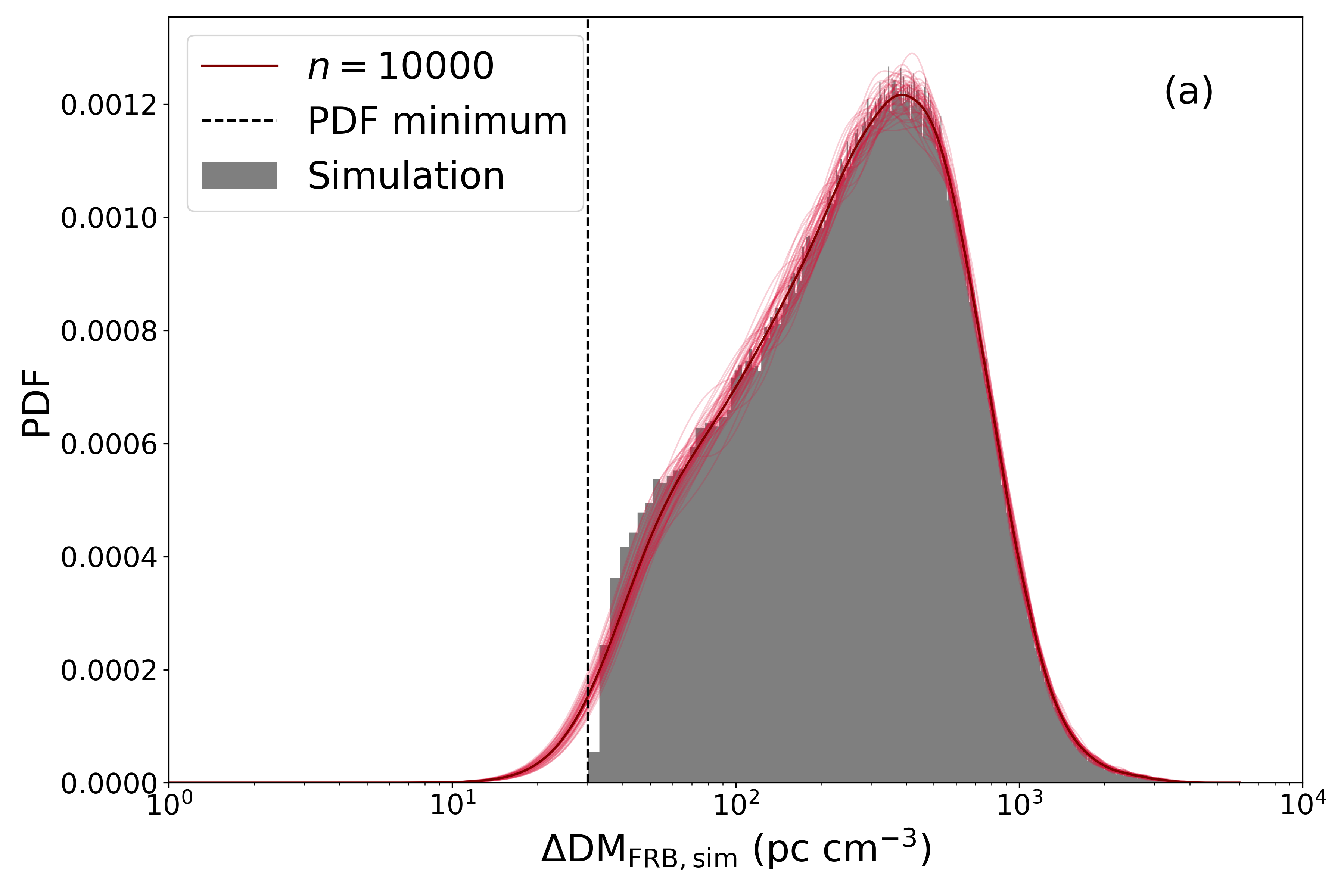
Figure 3a shows a realization of this simulated PDF for draws. This realization has an absolute minimum of and rises sharply due to the host and contributions. The dark red curve is the KDE (gamma) using the original data set and the other red curves are distributions generated with resampled data.
We explore the sensitivity of the analysis and results to samples size as follows. For and 10,000, we draw a random set of values and model the distributions with KDE (gamma). We then estimate a minimum value from the gradients of the PDFs, i.e. is the value which maximizes the slope of the KDE. Since each PDF is complemented by 1000 PDFs resampled from the original data set, 1000 minima are available for error estimation. The distribution of min[] values are shown in Table 3. As increases, the dispersion in min[] decreases and the central values approach (Figure 3b). Adding more than 10,000 samples has no notable effect on the results.
The simulation estimates are skewed to the left for small and approach a Gaussian distribution with increased confidence as increases (Figure 3b). While the mean values of the distributions are similar (Table 3), a sample size of is inadequate to place a constraint with reasonable confidence. The confidence level does however improve significantly as approaches 10,000.
Other choices for are explored to ensure the metric is reasonably robust to changes in the FRB simulation. Results are consistent, as detailed in § A. The smoother the leading edge of i.e. the smoother ), the more conservative the limits become, and a very sharp edge for i.e. a delta function for ) is described well by the metric. These cases represent extreme examples of possible host galaxy DM distributions.

| No. FRBs | ||
|---|---|---|
| 100 | ||
| 1000 | ||
| 10000 |
V Discussion
The principle empirical result of our work is a conservative upper limit on the DM contribution of the Milky Way halo. At , ( deg, YMW16). This can be converted to a conservative upper limit of (95% c.l.). This includes the ISM and halo, and potentially a non-zero contribution from the FRB host galaxy, which is plausibly several tens (see below). This limit also includes a non-zero contribution from the cosmic web (). That contribution is difficult to estimate at present but we note that the lowest redshift FRB (Marcote et al. 2020, ;) would yield an average of . A more realistic, yet speculative, upper limit to may therefore be .
The results presented include two measurements of uncertainty: systematic uncertainties related to ISM models and statistical uncertainties related to the estimation techniques. Another point to consider is the effect that Galactic latitude has on results. Owing to the complexity of the electron distribution at lower Galactic latitudes, we consider cuts of deg and deg. Results are largely insensitive to this cut, however the loss of data at deg (371 to 215 pulsars, and 83 to 64 FRBs), motivates a cut of deg for our final analysis.
Pulsar constraints are dominated by uncertainties in modeling . We find that, on average, values recovered from NE2001 are lower than those from YMW16. Given the expectation that , we use YMW16 in our analysis (see Table 2b). This gives a final result of (95% c.l.). We note that characterizing the line of sight to MW pulsars may help find HII regions that bias the estimate, allowing for improvement in the pulsar sample.
FRB constraints are predominantly limited by sample size , i.e., our simulations show a significant improvement as increases. For an absolute value of , limits for and 10,000 are , , and , respectively (95% c.l.). This suggests that once thousands of FRBs have been observed, the constraints will greatly improve.

Even the conservative limit of offers a valuable bound to models of the Galactic halo and the Local Group that our Galaxy resides within. Scenarios that adopt a Galactic halo mass which has retained all of its cosmic average of baryons estimate (Prochaska & Zheng 2019, but see Keating & Pen 2020). Furthermore, models which would predict the gas traces the dark matter profile would yield (Figure 4); these are ruled out by our FRB analysis, and also their over-estimated X-ray emission (Fang et al. 2015, e.g.). Our results also place an upper bound on the average contribution from the Local Group medium, consistent with current estimates (Prochaska & Zheng 2019). Clearly, as the observed FRB sample increases—one expects a dramatic leap from the CHIME survey (CHIME/FRB Collaboration et al. 2018)—the resultant limits may well distinguish between models where the Galaxy has retained the majority of its baryons from those where they have been expelled.
To illustrate the potential constraints, Figure 4 shows a model-based estimate for for a dark matter halo with mass , baryonic mass and that of those baryons are in a diffuse, ionized halo. The density profile is assumed to follow a modified Navarro-Frenk-White (NFW) profile parameterized by and (Mathews & Prochaska 2017; Prochaska & Zheng 2019, see). The upper limit to estimated from our analysis prefers larger with a strict NFW profile ( ruled out at high confidence unless . Larger are inferred for our Galaxy and external ones from absorption-line analyses (Faerman et al. 2017; Mathews & Prochaska 2017, e.g.).
We emphasize that ongoing FRB projects will offer complementary constraints on the magnitude and distribution of contributions from the host and the cosmic web to the upper limit on . In particular, well-localized FRBs reveal the host galaxy population and the redshift distribution of FRB events. From follow-up observations of the hosts, one may estimate the DM contribution from the host galaxy ISM through measurements of the Balmer line emission (Tendulkar et al. 2017; Chittidi et al. 2020, e.g.). The two systems analyzed thus far yield –. There are other FRBs (Bannister et al. 2019, e.g. FRB 180924; ) where the Balmer emission is low or even negligible at the FRB location and we infer . Within the next year, we expect to have a sample of hosts to derive the distribution.
One may additionally translate the estimated stellar mass of the host galaxy into a model-based estimate for the DM contribution from the halo gas of the host (Bannister et al. 2019; Prochaska & Zheng 2019). Current estimates range from for the most massive hosts (Bannister et al. 2019) to for FRB 181112 (Prochaska & Zheng 2019). From the redshift distribution of the localized FRBs, one may estimate the minimum typical contribution of to the limit. This bears an important caveat that the selection biases of the localized sample will not match those of the larger ensemble (e.g. due to differences in the radio frequencies and/or flux limit). One will need to account for these differences. Alternatively, one may focus on the analysis of the a localized sample alone once it grows to a sufficient sample size.
Last, we emphasize that other, future observations will also offer constraints on independent of FRB analyses. We anticipate high-precision X-ray absorption-line spectroscopy of the Galactic halo from the upcoming Japanese XRISM mission. With a spectral resolution that will greatly exceed current X-ray satellites, the data will yield much more reliable estimates of O+5 and O+6 column densities across the sky. At the least, these yield conservative lower limits to . Another promising yet still unrealized opportunity is to discover pulsars in Andromeda or any other Local Group galaxy. These would offer a strict upper bound on or even a well-informed value along that sightline.
VI Concluding Remarks
We have demonstrated how density estimation techniques can be used to probe the DM—i.e. the line-of-sight electron column density—of the MW Galactic halo. For the corrected and distributions, we recover and ( uncertainty). Conservative upper and lower limits on the Galactic halo dispersion measure are also derived: and (95% c.l.). Here the lower bound given by pulsars reflects only a fraction of the MW halo DM, and the upper bound given by FRBs includes a nominal contribution from the FRB host galaxy and IGM. In the latter case, the localization of FRBs at very low distances and/or on the outskirts of galaxies would establish that the minimum DM would be more representative of the MW halo. Scenarios consistent with this include the collapse of compact objects (Falcke & Rezzolla 2013, e.g.) that have been expelled from a host galaxy, as well as more exotic theories such as tiny electromagnetic explosions (Thompson 2017a; Thompson 2017b, which may occur in dark matter halos;) and cosmic strings (Vachaspati 2008; Yu et al. 2014; Zadorozhna 2015; Brandenberger et al. 2017, e.g.).
We do not consider how may vary as a function of Galactic latitude. It may be possible with a sample of a couple thousand FRBs per region of sky, but is left to future work.
Our current estimates cannot yet discern whether the Milky Way has retained its cosmic average of baryons (), however in the near future, as more FRBs are reported, results may offer a valuable complement to other analyses. In the least, the methodology provides a reasonable—albeit conservative—estimate of and a minimum contribution from . This may discern the viability of Galactic halo models and aid in the search for missing baryons.
References
- Bannister et al. (2019) Bannister, K. W., Deller, A. T., Phillips, C., et al. 2019, Science, 365, 565, doi: 10.1126/science.aaw5903
- Booth et al. (2012) Booth, C. M., Schaye, J., Delgado, J. D., & Dalla Vecchia, C. 2012, MNRAS, 420, 1053, doi: 10.1111/j.1365-2966.2011.20047.x
- Boylan-Kolchin et al. (2013) Boylan-Kolchin, M., Bullock, J. S., Sohn, S. T., Besla, G., & van der Marel, R. P. 2013, ApJ, 768, 140, doi: 10.1088/0004-637X/768/2/140
- Brandenberger et al. (2017) Brandenberger, R., Cyr, B., & Iyer, A. V. 2017. https://arxiv.org/abs/1707.02397
- Bregman et al. (2018) Bregman, J. N., Anderson, M. E., Miller, M. J., et al. 2018, ApJ, 862, 3, doi: 10.3847/1538-4357/aacafe
- Caleb et al. (2016) Caleb, M., Flynn, C., Bailes, M., et al. 2016, MNRAS, 458, 718, doi: 10.1093/mnras/stw109
- Chen (2000) Chen, S. X. 2000, Annals of the Institute of Statistical Mathematics, 52, 471, doi: 10.1023/A:1004165218295
- Chen et al. (2018) Chen, W.-C., Tareen, A., & Kinney, J. B. 2018, Phys. Rev. Lett., 121, 160605, doi: 10.1103/PhysRevLett.121.160605
- Cheng et al. (1997) Cheng, M.-Y., Fan, J., & Marron, J. S. 1997, The Annals of Statistics, 25, 1691. http://www.jstor.org/stable/2959068
- CHIME/FRB Collaboration et al. (2018) CHIME/FRB Collaboration, Amiri, M., Bandura, K., et al. 2018, ApJ, 863, 48, doi: 10.3847/1538-4357/aad188
- Chittidi et al. (2020) Chittidi, J., Simha, S., Mannings, A., et al. 2020, ApJ, accepted
- Coles (2001) Coles, S. 2001, An Introduction to Statistical Modeling of Extreme Values (Springer Series in Statistics. Berlin: Springer-Verlag), doi: https://doi.org/10.1007/978-1-4471-3675-0
- Cordes & Chatterjee (2019) Cordes, J. M., & Chatterjee, S. 2019, ARA&A, 57, 417, doi: 10.1146/annurev-astro-091918-104501
- Cordes & Lazio (2002) Cordes, J. M., & Lazio, T. J. W. 2002. https://arxiv.org/abs/astro-ph/0207156
- Cordes & Lazio (2003) —. 2003. https://arxiv.org/abs/astro-ph/0301598
- Cowling & Hall (1996) Cowling, A., & Hall, P. 1996, Journal of the Royal Statistical Society. Series B (Methodological), 58, 551. http://www.jstor.org/stable/2345893
- Dai et al. (2010) Dai, X., Bregman, J. N., Kochanek, C. S., & Rasia, E. 2010, ApJ, 719, 119, doi: 10.1088/0004-637x/719/1/119
- Faerman et al. (2013) Faerman, Y., Sternberg, A., & McKee, C. F. 2013, ApJ, 777, 119, doi: 10.1088/0004-637X/777/2/119
- Faerman et al. (2017) —. 2017, ApJ, 835, 52, doi: 10.3847/1538-4357/835/1/52
- Falcke & Rezzolla (2013) Falcke, H., & Rezzolla, L. 2013, Astronomy and Astrophysics, 562, doi: 10.1051/0004-6361/201321996
- Fang et al. (2013) Fang, T., Bullock, J. S., & Boylan-Kolchin, M. 2013, ApJ, 762, 20, doi: 10.1088/0004-637X/762/1/20
- Fang et al. (2015) Fang, T., Buote, D. A., Bullock, J. S., & Ma, R. 2015, ApJS, 217, 21, doi: 10.1088/0067-0049/217/2/21
- Faucher-Giguère & Kaspi (2006) Faucher-Giguère, C.-A., & Kaspi, V. M. 2006, ApJ, 643, 332, doi: 10.1086/501516
- Fukugita et al. (1998) Fukugita, M., Hogan, C. J., & Peebles, P. J. E. 1998, ApJ, 503, 518, doi: 10.1086/306025
- Gaensler et al. (2008) Gaensler, B. M., Madsen, G. J., Chatterjee, S., & Mao, S. A. 2008, PASA, 25, 184, doi: 10.1071/AS08004
- Gelman et al. (2014) Gelman, A., Carlin, J. B., Stern, H. S., & Rubin, D. B. 2014, Chapman & Hall, London, doi: 10.1111/j.1467-985X.2014.12096_1.x
- Hall & Wehrly (1991) Hall, P., & Wehrly, T. E. 1991, Journal of the American Statistical Association, 86, 665, doi: 10.1080/01621459.1991.10475092
- Henley et al. (2010) Henley, D. B., Shelton, R. L., Kwak, K., Joung, M. R., & Mac Low, M.-M. 2010, ApJ, 723, 935, doi: 10.1088/0004-637X/723/1/935
- Hoffmann & Jones (2015) Hoffmann, T., & Jones, N. S. 2015. https://arxiv.org/abs/1512.03188
- Jeon & Kim (2013) Jeon, Y., & Kim, J. H. 2013, Insurance: Mathematics and Economics, 53, 569, doi: 10.1016/j.insmatheco.2013
- Jones et al. (1996) Jones, M. C., Marron, J. S., & Sheather, S. J. 1996, Journal of the American Statistical Association, 91, 401, doi: 10.2307/2291420
- Keating & Pen (2020) Keating, L. C., & Pen, U.-L. 2020, Monthly Notices of the Royal Astronomical Society: Letters, doi: 10.1093/mnrasl/slaa095
- Kinney (2014) Kinney, J. B. 2014, Phys. Rev. E, 90, 011301, doi: 10.1103/PhysRevE.90.011301
- Kinney (2015) —. 2015, Phys. Rev. E, 92, 032107, doi: 10.1103/PhysRevE.92.032107
- Kocz et al. (2019) Kocz, J., Ravi, V., Catha, M., et al. 2019, MNRAS, 489, 919, doi: 10.1093/mnras/stz2219
- Kovács et al. (2019) Kovács, O. E., Bogdán, Á., Smith, R. K., Kraft, R. P., & Forman, W. R. 2019, ApJ, 872, 83, doi: 10.3847/1538-4357/aaef78
- Law et al. (2018) Law, C. J., Bower, G. C., Burke-Spolaor, S., et al. 2018, ApJS, 236, 8, doi: 10.3847/1538-4365/aab77b
- Lorimer et al. (2007) Lorimer, D. R., Bailes, M., McLaughlin, M. A., Narkevic, D. J., & Crawford, F. 2007, Science, 318, 777, doi: 10.1126/science.1147532
- Macquart (2018) Macquart, J.-P. 2018, Nature Astronomy, 2, 836, doi: 10.1038/s41550-018-0625-7
- Macquart & Ekers (2018) Macquart, J.-P., & Ekers, R. 2018, MNRAS, 480, 4211, doi: 10.1093/mnras/sty2083
- Manchester et al. (2006) Manchester, R. N., Fan, G., Lyne, A. G., Kaspi, V. M., & Crawford, F. 2006, ApJ, 649, 235, doi: 10.1086/505461
- Manchester et al. (2005) Manchester, R. N., Hobbs, G. B., Teoh, A., & Hobbs, M. 2005, AJ, 129, 1993, doi: 10.1086/428488
- Marcote et al. (2020) Marcote, B., Nimmo, K., Hessels, J. W. T., et al. 2020, Nature, 577, 190, doi: 10.1038/s41586-019-1866-z
- Mathews & Prochaska (2017) Mathews, W. G., & Prochaska, J. X. 2017, The Astrophysical Journal, 846, L24, doi: 10.3847/2041-8213/aa8861
- Müller & Wang (1994) Müller, & Wang, J.-L. 1994, Biometrics, 50, 61, doi: 10.2307/253319
- Müller (1991) Müller, H. 1991, Biometrika, 78, 521, doi: 10.1093/biomet/78.3.521
- Müller (1993) —. 1993, Scandinavian Journal of Statistics, 20, 313. http://www.jstor.org/stable/4616287
- Petroff et al. (2019) Petroff, E., Hessels, J. W. T., & Lorimer, D. R. 2019, Astron. Astrophys. Rev., 27, 4, doi: 10.1007/s00159-019-0116-6
- Petroff et al. (2016) Petroff, E., Barr, E. D., Jameson, A., et al. 2016, PASA, 33, e045, doi: 10.1017/pasa.2016.35
- Prochaska et al. (2011) Prochaska, J. X., Weiner, B., Chen, H.-W., Mulchaey, J., & Cooksey, K. 2011, ApJ, 740, 91, doi: 10.1088/0004-637X/740/2/91
- Prochaska & Zheng (2019) Prochaska, J. X., & Zheng, Y. 2019, MNRAS, 485, 648, doi: 10.1093/mnras/stz261
- Prochaska et al. (2019) Prochaska, J. X., Macquart, J.-P., McQuinn, M., et al. 2019, Science, doi: 10.1126/science.aay0073
- Ravi et al. (2019) Ravi, V., et al. 2019, Nature, 572, 352, doi: 10.1038/s41586-019-1389-7
- Ridley et al. (2013) Ridley, J. P., Crawford, F., Lorimer, D. R., et al. 2013, MNRAS, 433, 138, doi: 10.1093/mnras/stt709
- Riihimaki & Vehtari (2014) Riihimaki, J., & Vehtari, A. 2014, Bayesian Anal., 9, 425, doi: 10.1214/14-BA872
- Salem et al. (2015) Salem, M., Besla, G., Bryan, G., et al. 2015, ApJ, 815, 77, doi: 10.1088/0004-637X/815/1/77
- Schnitzeler (2012) Schnitzeler, D. H. F. M. 2012, MNRAS, 427, 664, doi: 10.1111/j.1365-2966.2012.21869.x
- Schuster (1985) Schuster, E. 1985, Communications in Statistics - Theory and Methods, 14, 1123, doi: 10.1080/03610928508828965
- Scott (1979) Scott, D. W. 1979, Biometrika, 66, 605, doi: 10.1093/biomet/66.3.605
- Silverman (1986) Silverman, B. W. 1986, Density Estimation for Statistics and Data Analysis (London: Chapman & Hall), doi: 10.1002/bimj.4710300745
- Skare et al. (2003) Skare, Ø., Bølviken, E., & Holden, L. 2003, Scandinavian Journal of Statistics, 30, 719, doi: 10.1111/1467-9469.00360
- Tendulkar et al. (2017) Tendulkar, S. P., et al. 2017, ApJ., 834, L7, doi: 10.3847/2041-8213/834/2/L7
- Thompson (2017a) Thompson, C. 2017a, ApJ, 844, 65, doi: 10.3847/1538-4357/aa7684
- Thompson (2017b) —. 2017b, ApJ, 844, 162, doi: 10.3847/1538-4357/aa7845
- Vachaspati (2008) Vachaspati, T. 2008, Phys. Rev. Lett., 101, 141301, doi: 10.1103/PhysRevLett.101.141301
- White & Rees (1978) White, S. D. M., & Rees, M. J. 1978, MNRAS, 183, 341, doi: 10.1093/mnras/183.3.341
- Yamasaki & Totani (2020) Yamasaki, S., & Totani, T. 2020, The Astrophysical Journal, 888, 105, doi: 10.3847/1538-4357/ab58c4
- Yao et al. (2017) Yao, J. M., Manchester, R. N., & Wang, N. 2017, ApJ, 835, 29, doi: 10.3847/1538-4357/835/1/29
- Yu et al. (2014) Yu, Y.-W., Cheng, K.-S., Shiu, G., & Tye, H. 2014, JCAP, 1411, 040, doi: 10.1088/1475-7516/2014/11/040
- Zadorozhna (2015) Zadorozhna, L. V. 2015, Advances in Astronomy and Space Physics, 5, 43, doi: 10.17721/2227-1481.5.43-50
Appendix A Minimum of FRB DM Distribution
We postulate that the minimum of the distribution can be approximated by . This metric is based on the prior that the underlying distribution has a sharp leading edge and is motivated by simulations. To bear weight, the metric must hold for a wide range of reasonable distributions.
The MW can be given by a delta function (as its DM is thought to vary by 10 ) and the cosmic DM distribution can be modelled theoretically. The distribution of host galaxy DMs, however, is unknown. In the main analysis we consider a lognormal distribution with and a standard deviation of . Here we consider two extreme variations: a delta function at and a broad Gaussian distribution with and . The former distribution makes the edge of sharper and the latter makes it smoother. The metric is a reasonable approximation for the combined contribution when each distribution is sharp (Figure 5a). When has a smooth edge, the estimates are more conservative (Figure 5b). Thus, provided the leading edge of is sufficiently sharp, the metric for determining the distribution minimum can be considered reasonably robust.
Looking at Figure 5, a sample size of appears sufficient to provide an estimate consistent with that of . For , distributions are wide and skewed to the left, providing results that are clearly premature.


Appendix B Density Estimation Using Field Theory
Density estimation using field theory (Kinney 2014; Kinney 2015; Chen et al. 2018, DEFT;) is a newly developed technique specifically developed for the small data regime. It takes a Bayesian field theory approach to density estimation in small data sets using a Laplace approximation of the Bayesian posterior (also see Riihimaki & Vehtari 2014). An advantage of DEFT over standard density estimation methods is that the method does not require the manual identification of critical parameters nor does it require the specification of boundary conditions. The DEFT simulations in this paper use the Python package SUFTware (Statistics Using Field Theory) by Chen et al. 2018.
Consider data points () drawn from a known probability distribution with intervals of length . We wish to find the best estimate of this distribution and the accompanying ensemble of other plausible estimates. Each distribution is parameterized by a real field , ensuring that is positive and normalized:
| (B1) |
Using scalar field theory, a prior is formulated that favours smooth probability densities. Specifically, Kinney 2015 consider priors of the form
| (B2) |
with action
| (B3) |
and partition function
| (B4) |
Here, gives the length scale below which fluctuations are strongly damped and is an integer in the range [1,…,4] that determines the smoothness. The resultant posterior is given by
| (B5) |
with nonlinear action
| (B6) |
and partition function
| (B7) |
is a histogram that summarizes the data.
Maximum a posteriori (MAP) density estimation approximates the posterior as a function given by the mode of the posterior, at which the action is then minimized. It has been shown that even without imposing boundary conditions on , has a unique minimum (Kinney 2015). The optimal length scale is identified by maximizing the Bayesian evidence .
The uncertainty in the DEFT estimate is determined by sampling the Bayesian posterior,
| (B8) |
by first drawing from and then drawing from . Laplace approximation is used to estimate by constructing a Gaussian centered at its MAP value. This gives the Laplace posterior,
| (B9) |
from which an ensemble of distributions can be sampled. Some of the s, however, are clearly not representative of the underlying distribution. Importance resampling is thus used to remove unfavorable distributions, where each is given a weight,
| (B10) |
proportional to its probability of being drawn (Chen et al. 2018). DEFT uses importance resampling with replacement, however for this work we invoke importance resampling without replacement.
When a posterior turns out to be a poor approximation of the target distribution, a few of the sampled distributions are given very large weights and the majority are given small weights (Gelman et al. 2014; Skare et al. 2003). When resampling with replacement, the heavily weighted distributions become significantly over represented. In our case, 60–70% of the sampled distributions were duplicates, which lead to notable bias when calculating the upper and lower bounds of . As such, we use a set of the most probable distributions, with limited replications. Specifically, we select 500 out of 1000 distributions via importance sampling without replacement. This lowered the duplication rate to .
We approximate the FRB distribution described in §IV.3 using DEFT for , and . Even for large DEFT is unable to adequately describe the sharp edge of the simulated distribution. In Figure 6a, the PDF tail extends below zero, violating the physical condition that . Further, the PDF cuts straight through the front of the simulated distribution and so bypasses the structure of the distribution’s edge.

Appendix C Generalized Extreme Value
A standard statistical technique for estimating the maximum values of an ensemble to fit it with a Generalized Extreme Value (GEV) PDF (Coles 2001, e.g.). This technique, however, is most applicable for assessing the upper limit of a distribution with a long tail. For , this holds for the largest values but the lowest values rise sharply as one may expect from the MW and host contributions.
Nevertheless, we attempted to estimate the minimum of following the standard practice of assessing the maximum of the negative of the distribution (Coles 2001). The results reported a minimum value at effectively infinite confidence at the lowest in the distribution and we found the results were unstable to random sampling.