Improved Computation-Communication Trade-Off for Coded Distributed Computing using Linear Dependence of Intermediate Values

We consider the problem of computing $Q$ output functions from $N$ input files. Given $N$ input files $w_{1},\ldots,w_{N}\in\mathbb{F}_{2^{F}}$, for some $F\in\mathbb{N}$, the goal is to compute $Q$ output functions $\phi_{1},\ldots,\phi_{Q}$, where $\phi_{q}:\left(\mathbb{F}_{2^{F}}\right)^{N}\to\mathbb{F}_{2^{B}},q\in\left\{1,\ldots,Q\right\}$. We assume that the output functions $\phi_{q},q\in\left\{1,\ldots,Q\right\}$ can be decomposed as follows:

where

• •

  The "Map" function $g_{q,n}:\mathbb{F}_{2^{F}}\to\mathbb{F}_{2^{T}}$ maps the input file $w_{n}$ into the length-$T$ intermediate value for some $T\in\mathbb{N}$. The intermediate value, which is the output of the map function $g_{q,n}$, is denoted by $v_{q,n}$, i.e., $v_{q,n}=g_{q,n}(w_{n})$.

• •

  The "Reduce" function $h_{q}:\left(\mathbb{F}_{2^{T}}\right)^{N}\to\mathbb{F}_{2^{B}}$ maps the intermediate values of the map functions into the output value.

The computation of map and reduce functions are carried out by $K$ distributed computing nodes (servers). They are interconnected through an error-free broadcast network.

Node $k$ computes the map functions of a set of files $\mathcal{M}_{k}\subseteq\left\{w_{1},\ldots,w_{N}\right\}$. The computation load is defined as $r\triangleq\frac{\sum_{k=1}^{K}|\mathcal{M}_{k}|}{N}$. For the sake of simplicity, we assume that the number of input files $N$ can be divided by $\binom{K}{r}$. In the map phase, the $N$ input files are evenly partitioned into $\binom{K}{r}$ disjoint batches of size $\eta_{1}=N/\binom{K}{r}$, each corresponding to a subset $\mathcal{T}\subset\left\{1,\ldots,K\right\}$ of size $r$, i.e.,

where $\mathcal{B}_{\mathcal{T}}$ denotes the batch of $\eta_{1}$ files corresponding to the subset $\mathcal{T}$. Node $k$ computes the map functions of the files in $\mathcal{B}_{\mathcal{T}}$ iff $k\in\mathcal{T}$.

Node $k$ computes a subset of output functions, whose indices are denoted by $\mathcal{W}_{k}\subseteq\left\{1,\ldots,Q\right\}$. Again, for the sake of simplicity, we assume that the number of the reduce functions $Q$ can be divided by $\binom{K}{s}$, and every subset of $s$ nodes reduce $Q/\binom{K}{s}$ functions. The parameter $s$ is the number of times each reduce function is computed. The $Q$ reduce functions are evenly partitioned into $\binom{K}{s}$ disjoint batches of size $\eta_{2}=Q/\binom{K}{s}$, each corresponding to a subset $\mathcal{P}$ of $s$ nodes, i.e.,

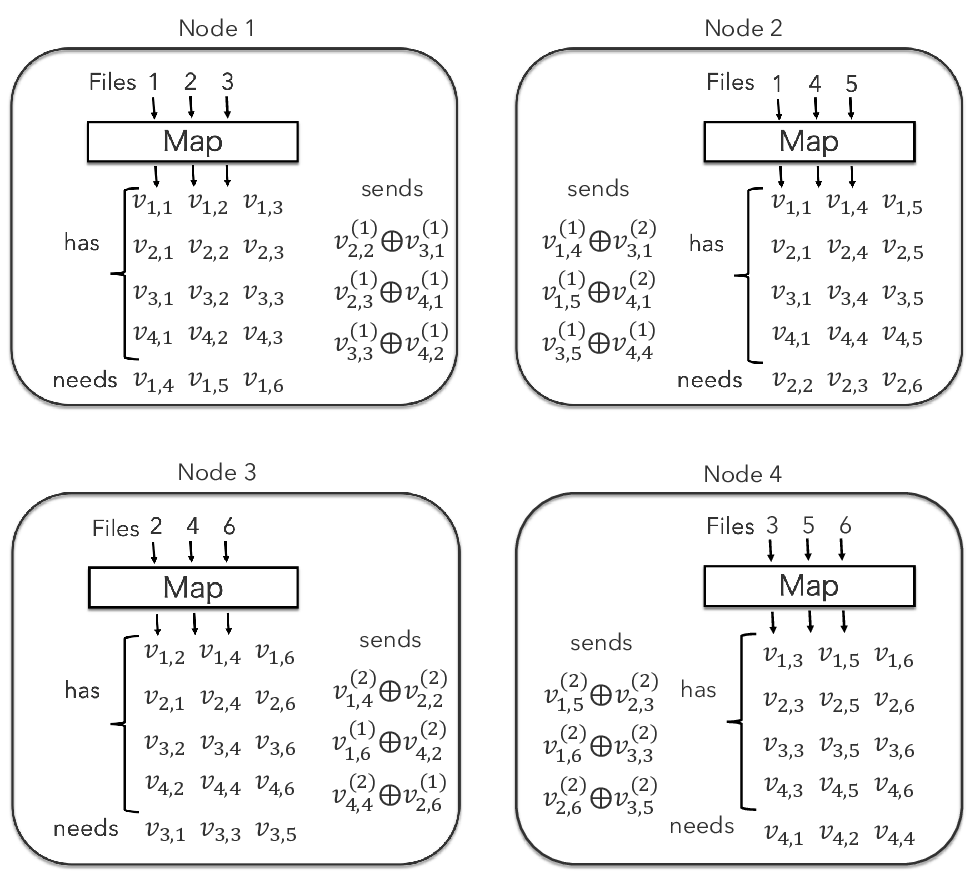
where $\mathcal{D}_{\mathcal{P}}$ denotes the indices of the batch of $\eta_{2}$ reduce functions corresponding to the subset $\mathcal{P}$. Node $k$ computes the reduce functions in the set $\mathcal{D}_{\mathcal{P}}$ iff $k\in\mathcal{P}$. An example of the distributed computing system is depicted in Fig. 1 for $K=4,N=6,Q=4,r=2,s=1$. For example, in this example, $\mathcal{B}_{\left\{1,2\right\}}=\left\{1\right\}$ and $\mathcal{D}_{\left\{1\right\}}=\left\{1\right\}$.

If the nodes are not allowed to utilize any coding scheme, each node has to receive the necessary intermediate values sent without coding by some other nodes. The communication load (the precise definition is given later) achieved by the uncoded scheme is

In the CDC scheme, the nodes construct the coded messages as follows. Let $\mathcal{S}$ be a subset of $\left\{1,\ldots,K\right\}$ of size $\max\left\{r+1,s\right\}\leq|\mathcal{S}|\leq\min\left\{r+s,K\right\}$. For a subset $\tilde{S}\subset\mathcal{S}$ with $|\tilde{\mathcal{S}}|=r$, let $\mathcal{V}_{\tilde{\mathcal{S}}}^{\mathcal{S}\setminus\tilde{\mathcal{S}}}$ be the set of intermediate values needed by all nodes in $\mathcal{S}\setminus\tilde{\mathcal{S}}$, not required by nodes outside $\mathcal{S}$, and known exclusively by nodes in $\tilde{\mathcal{S}}$, i.e.,

For example, $\mathcal{V}^{\left\{2\right\}}_{\left\{1,3\right\}}=\left\{v_{2,2}\right\}$ for the example in Fig. 1. The set $\mathcal{V}_{\tilde{\mathcal{S}}}^{\mathcal{S}\setminus\tilde{\mathcal{S}}}$ contains $\binom{r}{|\mathcal{S}|-s}\eta_{1}\eta_{2}$ intermediate values. A symbol $U_{\tilde{\mathcal{S}}}^{\mathcal{S}\setminus\tilde{\mathcal{S}}}\in\mathbb{F}_{2^{\binom{r}{|\mathcal{S}|-s}\eta_{1}\eta_{2}T}}$ is the concatenation of the intermediate values in $\mathcal{V}_{\tilde{\mathcal{S}}}^{\mathcal{S}\setminus\tilde{\mathcal{S}}}$. For $\tilde{\mathcal{S}}=\left\{\sigma_{1},\ldots,\sigma_{r}\right\}$, $U_{\tilde{\mathcal{S}}}^{\mathcal{S}\setminus\tilde{\mathcal{S}}}$ is split into $r$ segments, each containing $\binom{r}{|\mathcal{S}|-s}\frac{\eta_{1}\eta_{2}T}{r}$ bits, i.e.,

r example, $U^{\left\{2\right\}}_{\left\{1,3\right\},1}=v_{2,2}^{(1)}$ and $U^{\left\{2\right\}}_{\left\{1,3\right\},3}=v_{2,2}^{(2)}$, where $v_{2,2}^{(1)}$ and $v_{2,2}^{(1)}$ are the first half and second half bits of $v_{2,2}$, respectively. The node $\sigma_{i}\in\tilde{\mathcal{S}}$ is responsible for $U_{\tilde{\mathcal{S}},\sigma_{i}}^{\mathcal{S}\setminus\tilde{\mathcal{S}}}$. For each $k\in\mathcal{S}$, there are a total of $m_{\mathcal{S}}=\binom{|\mathcal{S}|-1}{r-1}$ subsets of $\mathcal{S}$ with size $r$ that contain the node $k$. We index these subsets as $\mathcal{S}_{(k)}[1],\ldots,\mathcal{S}_{(k)}[m_{\mathcal{S}}]$. Let $n_{\mathcal{S}}=\binom{|\mathcal{S}|-2}{r-1}$, then the the coded messages $\bm{X}_{k}^{\mathcal{S}}=(X_{k}^{\mathcal{S}}[1],\ldots,X_{k}^{\mathcal{S}}[n_{\mathcal{S}}])$, which are broadcast by the node $k$ to the nodes in $\mathcal{S}$ is constructed as follows.

where coefficients $a_{1},\ldots,a_{m_{\mathcal{S}}}\in\mathbb{F}_{2}^{\binom{r}{|\mathcal{S}|-s}}\frac{\eta_{1}\eta_{2}T}{r}$ are designed such that the nodes in $\mathcal{S}$ can decode the messages $\bm{X}_{k}^{\mathcal{S}}$. See [10] for detailed conditions. An example of the constructed message is depicted in Fig. 1. When $s=1$, only subsets of $\left\{1,\ldots,K\right\}$ of size $r+1$ are chosen as $\mathcal{S}$ and $A_{\mathcal{S}}=\left[1\ 1\ \ldots\ 1\right]$ for all $\mathcal{S}$, so the encoded messages are the XORs of some parts of the intermediate values.

The communication load is defined as $L\triangleq\frac{\sum_{k=1}^{K}b_{k}}{QNT}$, where $b_{k}$ is the number of bits sent by the node $k$. In [10], it is shown that the communication load of the coded scheme described above is

Especially, when $s=1$ (each reduce function is computed only once by a node), the communication load is given by

In [10], it is also shown that no scheme has smaller communication load for the same computation load if there is no further assumptions. However, as stated in the introduction, the map functions or reduce functions often have some structures in some applications. In such cases, the communication load may be further improved by utilizing these structures. In [13], it shows that the scheme that combines CDC scheme and compression scheme has better computation-communication trade-off when the reduce functions are linear aggregation, so this method utilizes the structure of the reduce functions. On the other hand, the method proposed in this paper utilizes the structure of the map functions.

Here, we present an illustrative example of the proposed scheme.

Consider a problem to counter the number of appearance of the numbers in the following sequence.

The sequence has 4 numbers. We consider a distributed computing system with $K=4,N=6$, where the input files $w_{1},\ldots,w_{6}$ are the 6 blocks of the sequence each of length 7. We assume that the node $k$ counts the number of appearance of the number $k$. Then, the intermediate value $v_{q,n}$ represents the number of ’$q$’s in the $n$-th block of the sequence. For example, $v_{1,1}=3,v_{1,2}=5,v_{1,3}=3$. Consider the CDC scheme presented in the previous section with $r=2$, which is the same as the example presented in Fig. 1. Then, the node broadcasts $v_{2,2}^{(1)}\oplus v_{3,1}^{(1)}$, $v_{2,3}^{(1)}\oplus v_{4,1}^{(1)}$ and $v_{3,3}^{(1)}\oplus v_{4,2}^{(1)}$. Since $v_{2,3}=v_{3,3}=2$ and $v_{4,1}=v_{4,2}=0$, it holds $v_{2,3}\oplus v_{4,1}=v_{3,3}\oplus v_{4,2}$. As a consequence, it also holds $v_{2,3}^{(1)}\oplus v_{4,1}^{(1)}=v_{3,3}^{(1)}\oplus v_{4,2}^{(1)}$. This fact indicates that the rank of the subspace constructed from 3 coded messages is 2. Thus, it is sufficient for the node 1 to broadcast the 2 basis vectors and their linear combination coefficients. Since it requires 2 linear combination coefficients in $\mathbb{F}_{2}$ for each coded message, the number of bits sent by the node 1 is $2\cdot\frac{T}{2}+3\times 2=T+6$, which is smaller than $\frac{3T}{2}$, the number of bits required to send the message in the original form, when $T$ is larger than 12¹¹ 1 This is not the case for the example because $T=6$ is sufficient for representing the coded messages. However, $T$ would take very large values for big data applications.. This is because the dimension of the subspace constructed from the messages is smaller than the number of messages. This example can be considered as a special case of the problem of word count in a large document. In many cases, many words do not appear or appear only a small number of times in the divided blocks of the document. In such cases, many intermediate values would have the same value, resulting in a smaller subspace rank.

Next example is the problem to compute linear transforms of high-dimensional vectors, which is a critical step in several machine learning and signal processing applications. Consider a problem to compute linear transforms in which given a matrix $\bm{A}\in\mathbb{F}_{q}^{m\times n}$ and $N$ input vectors $\bm{x}_{1},\ldots,\bm{x}_{N}\in\mathbb{F}_{q}^{n}$, we want to compute $\bm{y}_{1}=\bm{A}\bm{x}_{1},\ldots,\bm{y}_{N}=\bm{A}\bm{x}_{N}$. We consider the problem to compute these linear transforms in a distributed computing system with $K$ nodes. There are various ways to compute the linear transforms in a distributed manner. One of such methods is that the matrix $A$ is divided by rows into submatirices $\left\{\bm{A}_{k}:k=1,\ldots,K\right\}$ and the linear functions defined by $\bm{A}_{k},k=1,\ldots,K$ are regarded as the reduce functions. Each server $k$ computes some of $\left\{A_{k}\bm{x}_{i}:i=1,\ldots,N\right\}$ and these output vectors are the intermediate values. In this case, each intermediate value is represented by $T=m\log_{2}q/K$ bits. Consider the case where $s=1$, that is, each reduce function is computed only once by a node. Then, the length of the encoded messages is $\frac{mN\log_{2}q}{rK\binom{K}{r}}$ and the number of the messages sent by a node is $\binom{K}{r+1}$. The rank of the subspace constructed from the encoded messages is smaller than or equal to $\min\left\{\frac{mN\log_{2}q}{rK\binom{K}{r}},\binom{K}{r+1}\right\}$ and it is smaller than the number of messages $\binom{K}{r+1}$ for some cases. For a system with $K=Q=16,N=128$ and a problem with $q=2,m=2048$, the relation between the length and the number of the encoded messages sent by a node is depicted in Fig. 2.

In some cases, the rank of the subspace is even smaller. For example, as in [2], one may construct the submatrices $\left\{\bm{A}_{k}:k=1,\ldots,K\right\}$ so that each submatrix is sparse. Furthermore, in machine learning applications, vectors $\bm{x}_{1},\ldots,\bm{x}_{N}$ are often sparse [14]. Then, the intermediate values are zero vectors with high probability and they are linearly dependent.

Another example is also the problem to compute linear transforms of high-dimensional vectors, but in a situation that there would be some straggling nodes in the system. For this problem, the scheme that combines the CDC scheme and error-correcting codes are proposed in [11, 12]. In these schemes, error-correcting linear codes are applied to the matrix $\bm{A}$ and each server $k$ stores

where $\bm{E}_{1},\ldots,\bm{E}_{K}$ are designed so that the system can compute $\bm{A}\bm{x}$ even if some straggling nodes exist. Each server $k$ compute some of $\left\{\bm{U}_{k}\bm{x}_{i}:i=1,\ldots,N\right\}$. From the construction, $\bm{U}_{1},\ldots,\bm{U}_{K}$ are linearly dependent. As a consequence, the intermediate values are also linearly dependent.

The only difference of the proposed scheme from the scheme presented in section III is the way to construct the coded message in the shuffle phase. First, each node compute the coded messages of the intermediate values in the same way as in (7). Each $\bm{X}_{k}^{\mathcal{S}}$ is a length-$\binom{|\mathcal{S}|-2}{r-1}\binom{r}{|\mathcal{S}|-s}\frac{\eta_{1}\eta_{2}T}{r}$ binary vector. For $\max\left\{r+1,s\right\}\leq\ell\leq\min\left\{r+s,K\right\}$, there are a total of $\binom{K-1}{\ell-1}$ subsets of $\left\{1,\ldots,K\right\}$ with size $\ell$ that contain the node $k$. Consider a set of messages

The set contains $\binom{K-1}{\ell-1}$ of length-$\binom{\ell-2}{r-1}\binom{r}{\ell-s}\frac{\eta_{1}\eta_{2}T}{r}$ vectors. This set can be considered as a linear subspace. Let $\rho_{k,\ell}$ be the rank of the subspace (12). The node $k$ computes the $\rho_{k,\ell}$ basis of the subspace and send the basis and linear combination coefficients which are needed to recover the original coded messages. We call the proposed scheme CDC-LD. Since each node send $\binom{K-1}{\ell-1}$ coded messages and it requires $\rho_{k,\ell}$ linear combination coefficients in $\mathbb{F}_{2}$ to express each of them, the number of the bits sent by node $k$ is $\rho_{k,\ell}\binom{\ell-2}{r-1}\binom{r}{\ell-s}\frac{\eta_{1}\eta_{2}T}{r}+\rho_{k,\ell}\binom{K-1}{\ell-1}=\left(\binom{\ell-2}{r-1}\binom{r}{\ell-s}\frac{\eta_{1}\eta_{2}T}{r}+\binom{K-1}{\ell-1}\right)\rho_{k,\ell}$. As $\ell$ varies from $\max\left\{r+1,s\right\}\leq\ell\leq\min\left\{r+s,K\right\}$, the proposed scheme has the following performance.

The communication load of the proposed scheme depends on the values of $Q,T,\rho_{\ell}$, while the original scheme does not. Therefore, it depends on these values whether the proposed scheme is more efficient than the original scheme. The communication loads of the original scheme and the proposed scheme are depicted in Fig. 3 for different values of $T$, where $K=4,N=6,Q=4,r=2,s=1$. We can see that the communication load of the proposed system decreases as the length $T$ of the intermediate values increases. In this case, the proposed scheme has better performance compared to the original scheme provided that $T\geq 12$ and the average rank $\rho_{\ell}\leq 2$.

Fig. 4 shows the trade-off relationship between the computation load and the communication load for the system with $K=10,N=2520,Q=360,T=64$. We can see that the computation load is a medium value, the proposed methods perform better than the original scheme.

The proposed system utilizes the structure of the map functions and no assumptions are put for the reduce functions. So we can combine the proposed method with the method proposed in [13] if the map functions have some linear dependent structure and the reduce functions are the linear aggregation where the reduce function is the sum of intermediate values.

Our proposed method can be considered as one of the methods of compressing the intermediate values. Therefore, the lower bound of the communication load of each server to send its intermediate value is given by its entropy. However, coding schemes with good compression performance often have large computational complexity for coding and decoding, resulting in an increase in the computational time of the overall system. In our proposed scheme, it has to compute the basis of the subspace. Although its computation cost is very high in some cases, there are some cases that it is not so high. For example, we can choose standard basis for the problem of computing linear transforms. In those cases, we can obtain a cost-effective improvement.

References

- [1] K. Lee, M. Lam, R. Pedarsani, D. Papailiopoulos, and K. Ramchandran, “Speeding up distributed machine learning using codes,” IEEE Transactions on Information Theory, vol. 64, no. 3, pp. 1514–1529, 2018.
- [2] S. Dutta, V. Cadambe, and P. Grover, “Short-dot: Computing large linear transforms distributedly using coded short dot products,” in Advances In Neural Information Processing Systems, 2016, pp. 2100–2108.
- [3] Q. Yu, M. Maddah-Ali, and S. Avestimehr, “Polynomial codes: an optimal design for high-dimensional coded matrix multiplication,” in Advances in Neural Information Processing Systems, 2017, pp. 4403–4413.
- [4] C. Karakus, Y. Sun, S. Diggavi, and W. Yin, “Straggler mitigation in distributed optimization through data encoding,” in Advances in Neural Information Processing Systems, 2017, pp. 5434–5442.
- [5] R. Tandon, Q. Lei, A. G. Dimakis, and N. Karampatziakis, “Gradient coding: Avoiding stragglers in distributed learning,” in International Conference on Machine Learning, 2017, pp. 3368–3376.
- [6] S. Li, S. M. M. Kalan, A. S. Avestimehr, and M. Soltanolkotabi, “Near-optimal straggler mitigation for distributed gradient methods,” in 2018 IEEE International Parallel and Distributed Processing Symposium Workshops (IPDPSW). IEEE, 2018, pp. 857–866.
- [7] M. Ye and E. Abbe, “Communication-computation efficient gradient coding,” in International Conference on Machine Learning, 2018, pp. 5606–5615.
- [8] W. Halbawi, N. Azizan, F. Salehi, and B. Hassibi, “Improving distributed gradient descent using reed-solomon codes,” in 2018 IEEE International Symposium on Information Theory (ISIT). IEEE, 2018, pp. 2027–2031.
- [9] S. Horii, T. Yoshida, M. Kobayashi, and T. Matsushima, “Distributed stochastic gradient descent using ldgm codes,” in 2019 IEEE International Symposium on Information Theory (ISIT), July 2019, pp. 1417–1421.
- [10] S. Li, M. A. Maddah-Ali, Q. Yu, and A. S. Avestimehr, “A fundamental tradeoff between computation and communication in distributed computing,” IEEE Transactions on Information Theory, vol. 64, no. 1, pp. 109–128, 2017.
- [11] S. Li, M. A. Maddah-Ali, and A. S. Avestimehr, “A unified coding framework for distributed computing with straggling servers,” in 2016 IEEE Globecom Workshops (GC Wkshps). IEEE, 2016, pp. 1–6.
- [12] J. Zhang and O. Simeone, “Improved latency-communication trade-off for map-shuffle-reduce systems with stragglers,” in ICASSP 2019-2019 IEEE International Conference on Acoustics, Speech and Signal Processing (ICASSP). IEEE, 2019, pp. 8172–8176.
- [13] S. Li, M. A. Maddah-Ali, and A. S. Avestimehr, “Compressed coded distributed computing,” in 2018 IEEE International Symposium on Information Theory (ISIT). IEEE, 2018, pp. 2032–2036.
- [14] J. Duchi, E. Hazan, and Y. Singer, “Adaptive subgradient methods for online learning and stochastic optimization,” Journal of Machine Learning Research, vol. 12, no. Jul, pp. 2121–2159, 2011.