Estimating the integral length scale on turbulent flows from the zero crossings of the longitudinal velocity fluctuation

For this study, we employed a Reynolds decomposition for the streamwise velocity ($u=U+u^{\prime}(\tau)$ ), to extract the eulerian fluctuating velocity $u^{\prime}$. We then computed the fluctuating velocity $u^{\prime}(\tau)$ zero crossings, i.e., the set of times $\tau^{c}_{i}$ for which $u^{\prime}(\tau^{c}_{i})=0$ (see top of figure 1(b)), and translated this list of zero crossings from time into space by assuming the Taylor hypothesis $Z_{i}=\tau^{c}_{i}U$ (see figure 1(b)). It was verified that all measurements had enough temporal resolution to estimate $\lambda$ MoraPRF2019 via the zero crossings. A common procedure to verify the latter sreenivasan1983zero; mazellier2008turbulence is as follows:

1. 1.

   Take the acquired fluctuating velocity signal, and low pass filter it (with a high order filter, e.g. a fifth order butterworth filter) at different sizes $\eta_{C}=2\pi/\kappa$ (where $\kappa$ is the wave number), given the use of the Taylor hypothesis this is equivalent to filter at different frequencies.

2. 2.

   Compute the signal zero crossings, and their number density ($n_{s}=$number of zeros/duration of the signal) at at each filter size (frequency).

3. 3.

   If a plateau of $n_{s}$ is present for filter scales smaller (larger) than a certain scale (frequency) $\eta_{C}^{\star}$ (not to be confused with the Kolmogorov length scale $\eta$), the value of $n_{s}$ is properly resolved. One could then estimate $\lambda$ via $n_{s}^{-1}|_{\star}=\pi C\lambda$, with $C$ being a constant in the order of unity which accounts for the non-gaussianity of the signal mazellier2008turbulence.

The seminal work of McFadden mcfadden1958axis was the first to derive for gaussian processes closed expressions to compute the variance of the interval distance between two successive zero crossings ($\Delta Z=Z_{i+1}-Z_{i}$) under two analytically tractable conditions: intervals between zeros are statistically independent, or intervals between zeros make a Markov chain. For the former, statistically independent case, the expression for the variance goes as,

The latter expression, and assuming Taylor hypothesis, provides an estimate for $\mathcal{L}$ if the assumption of independent zero crossing intervals approximately holds for turbulent signals;

By truncating the integral up to the first term, one obtains a relation between the Fano factor smith2008fluctuations, and the integral time ($\mathcal{T}$) and length scales:

Interestingly, if McFadden’s assumption of statistically independent intervals holds, the variance of the length between two successive intervals bendat2011random could be written as,

Thus, an easy way to analyse the implications of this assumption (and its deviations) could be using 1D Voronoï tessellations ferenc2007size. These two frameworks (Voronoï tessellations and ‘raw’ inter-crossing distances) are related by their respective definitions. For instance, if a random variable $\Delta Z$ represents the distance between successive crossings, the respective Voronoï cell length $L$ (also a random variable) is given by $L=1/2(\Delta Z_{L}+\Delta Z_{R})$, where $\Delta Z_{L}=|Z_{P}-Z_{L}|$ and $\Delta Z_{R}=|Z_{R}-Z_{P}|$ are the crossing lengths (random variables) at the left, and at the right of the crossing $Z_{P}$ (see figure 1(b)). From these definitions; $\langle L\rangle=\langle\Delta Z\rangle=n^{-1}_{s}$.

Then, if the covariance between $\Delta Z_{L}$ and $\Delta Z_{R}$ is very weak, the variance of the ensemble of normalized Voronoï cells ($\mathcal{V}=L/\langle L\rangle$) is half the variance of $\Delta Z/\langle\Delta Z\rangle^{2}$:

The latter expression is easily verified for a random Poisson process (RPP), for which $\langle\Delta Z\rangle=1$, $\mathrm{Var}(\Delta Z)=1$, and its respective Voronoï normalised cell variance is $\mathrm{Var}(L)/\langle L\rangle^{2}=1/2$ ferenc2007size. We will refer to the standard deviation of this RPP process as $\sigma_{RPP}=\sqrt{1/2}$, and to the respective standard deviation coming from our Voronoï analysis of turbulent signals as $\sigma_{\mathcal{V}}$.

We compute the values of $\mathrm{Var}(\Delta Z)$ and $\langle\Delta Z\rangle$ for all datasets and examine the accuracy of McFadden’s equation (equation 3). To estimate $\mathrm{Var}(\Delta Z)$ and $\langle\Delta Z\rangle$, we follow a standard procedure found in the literature sreenivasan1983zero; mazellier2008turbulence, and described in section 2.1: we low-pass filter $u^{\prime}$ with a range of filter sizes $\eta_{C}$, and compute the signal zero crossings and zero crossings density at each filter size. The presence of a plateau (not reported here, but present for all our datatets) for small values of $\eta_{C}$ show that $n_{s}$ is well resolved, and therefore $\lambda$ can be computed as $n^{-1}_{s}=\langle\Delta Z\rangle\sim\pi\lambda$. Resolving $\lambda$ gives credence to the use of McFadden’s equation with our datasets values.

To check the validity of McFadden’s equation, we apply it to all velocity signals and for all filter scales (see figure 2). The equation provides indeed an acceptable estimation of $\mathcal{L}$ for large values of $Re_{\lambda}$ when the value at the plateau is compared to the traditional method of integrating up to the first zero of the autocorrelation.

Our method, however, has a residual dependency on $Re_{\lambda}$ coming from variance value at the plateau, and as expected from previous analyses mazellier2008turbulence. On the other hand, for the AG data (figure 2(d)), our results suggest that there was indeed a underestimation of the original values of $\mathcal{L}=\int_{0}^{r_{0}}\rho(r)dr$ (already discussed in MoraPRF2019), and such underestimation strongly depends on the value of $\delta$ selected; as $\delta$ increases $\mathcal{L}$ decreases.

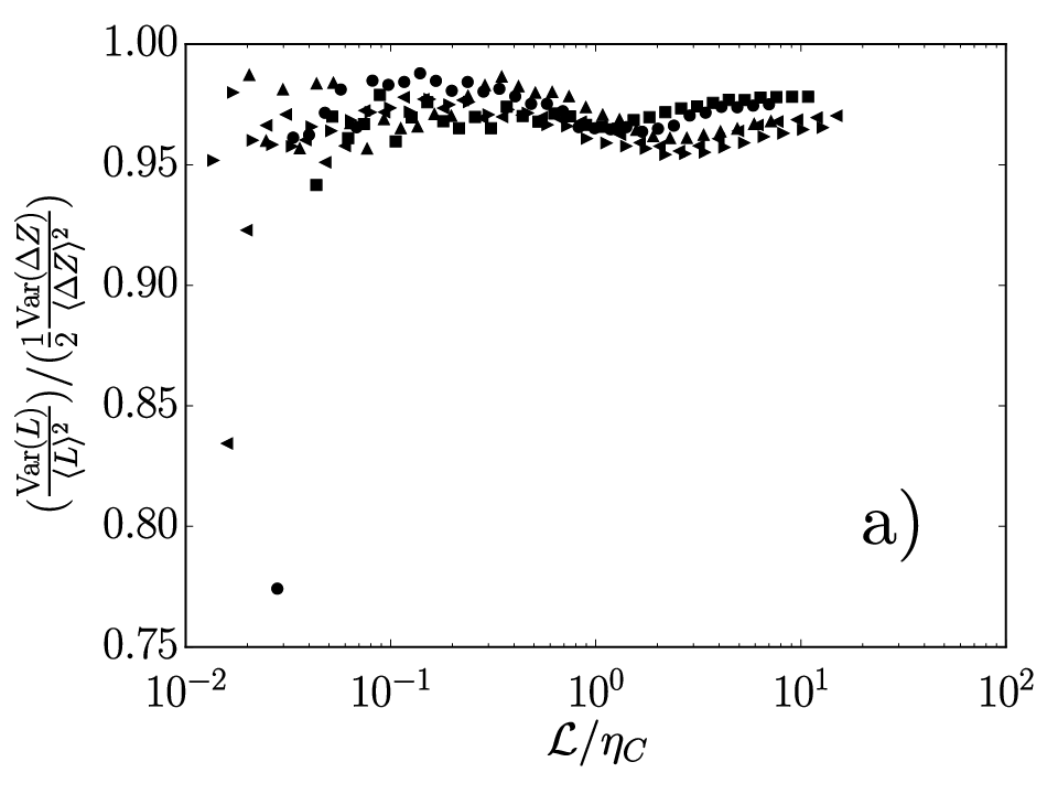
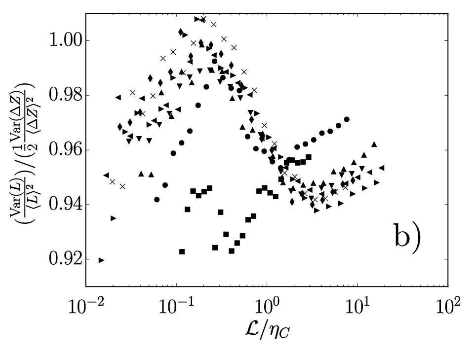
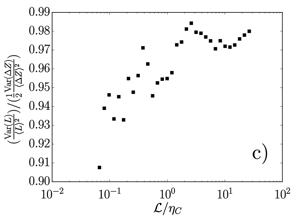
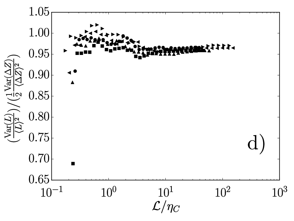
Moreover, these observations advance that indeed the assumption of independent successive zero crossings could hold to some extent in turbulent signals. In fact, if equation 4 is approximately valid at all filters of interest, then the same follows for equation 5 , which relates the variance of the Voronoï tessellation $\sigma_{\mathcal{V}}^{2}$ applied to zero crossings with the variance of the interval distance between two successive zero crossings $\mathrm{Var}(\Delta Z)$. The latter yields $\mathrm{Var}(L)=\frac{1}{2}\mathrm{Var}(\Delta Z)$. Equation 5 then (see figures 3(a) to 3(d)) gives:

at all filter scales of interest for the data found in Table 1. This observation supports that the independent interval assumption is approximately valid within $10\%$ error for our datasets.

Taking into account the previous section observations, we applied 1D Voronoï tessellation analysis ferenc2007size to the signals’ zero crossings (see figure 1(b)) at each filter scale.

Our results reveal that $\sigma_{\mathcal{V}}$ (see figures 4(a) to 4(d)) has complex behaviour with the filter scale $\eta_{C}$ which can be divided in 3 parts. First, a plateau regime at low values of $\kappa_{C}\sim\eta_{C}^{-1}$ representative of a flat white noise gaussian spectrum. Second, an intermediate regime where $\sigma_{\mathcal{V}}$ may attain a power law behaviour with an exponent close to $1/4$ for large values of $Re_{\lambda}$; despite of its persistence among different datasets, the existence of this intermediate regime remains unexplained and is left for future research as the limited extend of our data does not allows us to unambiguously conclude the accuracy of the exponent. Third, a second plateau consistent with the one found for the zero crossing number density $n^{-1}_{s}=\langle\Delta Z\rangle$ is found.

On the contrary, and interestingly, there seems to be a strong correlation between the filter scale at which $\sigma_{\mathcal{V}}/\sigma_{RPP}\approx 1$, and $\mathcal{L}$, i.e., apparently $\sigma_{\mathcal{V}}/\sigma_{RPP}\approx 1$ when $\eta_{C}=\mathcal{L}$. These results hint that an alternative definition of $\mathcal{L}$ could be: the length-scale at which the zero crossing intervals topology is approximately uncorrelated.

Furthermore, a comparison between the values estimated from McFadden’s equation (taking the last points of the plateaus of $n_{s}$, and $\sigma_{\mathcal{V}}$), and the values extracted from $\sigma_{\mathcal{V}}/\sigma_{RPP}\approx 1$ when $\eta_{C}=\mathcal{L}$ (see figures 2(d) and 5(a)) points out again that for the AG data, the integral length scale $\mathcal{L}$ could have been originally underestimated by a factor of 2 explaining the discrepancy in $C_{\varepsilon}$ between the studies of MoraPRF2019, and puga2017normalized. This underestimation occurs, when integrating the autocorrelation by the method proposed by puga2017normalized, as a consequence of the arbitrary choice of the value $\delta$; smaller values converge to a closer value of $\mathcal{L}$, while larger values of $\delta$ reduce the noise while keeping the trends.

These observations suggest that the integral length scale can also be estimated as $\mathcal{L}=\mathcal{L}_{Voro}=\eta_{C}|_{\sigma_{\mathcal{V}}\approx\sigma_{RPP}}$. This new definition (see figure 5(b)) seems to be less sensitive to $Re_{\lambda}$ than the value of $\mathcal{L}$ estimated from equation 3, and to have less dispersion. The values obtained by the latter method show that for grid turbulence at large $U_{\infty}$, $\mathcal{L}$ increases with $Re_{\lambda}$, as previously reported.

On the other hand, and in the context of inertial particles clustering, Monchaux et al. Monchaux2010 introduced Voronoï tessellations, and argued that clustering is present when the ratio $\sigma_{\mathcal{V}}|_{\star}/\sigma_{RPP}>1$ (where $\sigma_{\mathcal{V}}|_{\star}$ is the value of $\sigma_{\mathcal{V}}$ at the plateau observed at small values of $\eta_{C}$), and its intensity depends on this ratio magnitude. Being the standard deviation mainly set by the ‘voids’ sumbekova2017preferential (periods without zero crossings ), our results show that the degree of clustering of zero crossings increases with $Re_{\lambda}^{1/3}$ (see figure 5(c)), in agreement with the observations of Mazellier and Vassilicos mazellier2008turbulence.

We therefore conclude that while McFadden’s equation gives a good estimation of $\mathcal{L}$, a better estimation could be $\mathcal{L}=\eta_{C}|_{\sigma_{\mathcal{V}}=\sigma_{RPP}}$. The last expression relies on the same hypotheses as McFadden’s model, and still has the advantage of producing the value of $\mathcal{L}$ even for non-stationary or non-calibrated data.

References

- (1) Bendat, J.S., Piersol, A.G.: Random data: analysis and measurement procedures, vol. 729. John Wiley & Sons (2011)
- (2) Bewley, G.P., Chang, K., Bodenschatz, E., for Turbulence Research), I.C.: On integral length scales in anisotropic turbulence. Physics of Fluids 24(6), 061702 (2012)
- (3) Cava, D., Katul, G.G., Molini, A., Elefante, C.: The role of surface characteristics on intermittency and zero-crossing properties of atmospheric turbulence. Journal of Geophysical Research: Atmospheres 117(D1) (2012)
- (4) Chamecki, M.: Persistence of velocity fluctuations in non-gaussian turbulence within and above plant canopies. Physics of Fluids 25(11), 115110 (2013)
- (5) Dairay, T., Obligado, M., Vassilicos, J.C.: Non-equilibrium scaling laws in axisymmetric turbulent wakes. Journal of Fluid Mechanics 781, 166–195 (2015)
- (6) Davila, J., Vassilicos, J.: Richardson’s pair diffusion and the stagnation point structure of turbulence. Physical review letters 91(14), 144501 (2003)
- (7) Ferenc, J.S., Néda, Z.: On the size distribution of poisson voronoi cells. Physica A: Statistical Mechanics and its Applications 385(2), 518–526 (2007)
- (8) Gagne, Y., Castaing, B., Baudet, C., Malécot, Y.: Reynolds dependence of third-order velocity structure functions. Physics of Fluids 16(2), 482–485 (2004)
- (9) Griffin, K.P., Wei, N.J., Bodenschatz, E., Bewley, G.P.: Control of long-range correlations in turbulence. Experiments in Fluids 60(4), 55 (2019)
- (10) Hearst, R.J., Lavoie, P.: The effect of active grid initial conditions on high reynolds number turbulence. Experiments in Fluids 56(10), 185 (2015)
- (11) Krogstad, P.Å., Davidson, P.: Freely decaying, homogeneous turbulence generated by multi-scale grids. Journal of fluid mechanics 680, 417–434 (2011)
- (12) Mazellier, N., Vassilicos, J.: The turbulence dissipation constant is not universal because of its universal dependence on large-scale flow topology. Physics of Fluids 20(1), 015101 (2008)
- (13) McFadden, J.: The axis-crossing intervals of random functions–ii. IRE Transactions on Information Theory 4(1), 14–24 (1958)
- (14) Monchaux, R., Bourgoin, M., Cartellier, A.: Preferential concentration of heavy particles: A Voronoï analysis. Physics of Fluids 22(10) (2010). DOI 10.1063/1.3489987
- (15) Mora, D.O., Cartellier, A., Obligado, M.: Experimental estimation of turbulence modification by inertial particles at moderate . Phys. Rev. Fluids 4, 074309 (2019). DOI 10.1103/PhysRevFluids.4.074309. URL https://link.aps.org/doi/10.1103/PhysRevFluids.4.074309
- (16) Mora, D.O., Muñiz Pladellorens, E., Riera Turró, P., Lagauzere, M., Obligado, M.: Energy cascades in active-grid-generated turbulent flows. Phys. Rev. Fluids 4, 104601 (2019). DOI 10.1103/PhysRevFluids.4.104601. URL https://link.aps.org/doi/10.1103/PhysRevFluids.4.104601
- (17) Mydlarski, L.: A turbulent quarter century of active grids: from makita (1991) to the present. Fluid Dynamics Research 49(6), 061401 (2017)
- (18) O’Neill, P.L., Nicolaides, D., Honnery, D., Soria, J., et al.: Autocorrelation functions and the determination of integral length with reference to experimental and numerical data. In: 15th Australasian fluid mechanics conference, vol. 1, pp. 1–4. Univ. of Sydney Sydney, NSW, Australia (2004)
- (19) Orey, S.: Gaussian sample functions and the hausdorff dimension of level crossings. Zeitschrift für Wahrscheinlichkeitstheorie und verwandte Gebiete 15(3), 249–256 (1970)
- (20) Pope, S.B.: Turbulent Flows. Cambridge University Press (2000)
- (21) Puga, A.J., LaRue, J.C.: Normalized dissipation rate in a moderate taylor reynolds number flow. Journal of Fluid Mechanics 818, 184–204 (2017)
- (22) Smith, J., Hopcraft, K., Jakeman, E.: Fluctuations in the zeros of differentiable gaussian processes. Physical Review E 77(3), 031112 (2008)
- (23) Sreenivasan, K., Prabhu, A., Narasimha, R.: Zero-crossings in turbulent signals. Journal of Fluid Mechanics 137, 251–272 (1983)
- (24) Sumbekova, S., Cartellier, A., Aliseda, A., Bourgoin, M.: Preferential concentration of inertial sub-Kolmogorov particles: The roles of mass loading of particles, Stokes numbers, and Reynolds numbers. Physical Review Fluids 2(2), 24302 (2017). DOI 10.1103/PhysRevFluids.2.024302
- (25) Tennekes, H., Lumley, J.L.: A first course in turbulence. MIT press (1972)
- (26) Tritton, D.J.: Physical fluid dynamics. Springer Science & Business Media (2012)
- (27) Valente, P., Vassilicos, J.C.: The decay of turbulence generated by a class of multiscale grids. Journal of Fluid Mechanics 687, 300–340 (2011)
- (28) Vassilicos, J.C.: Dissipation in turbulent flows. Annual Review of Fluid Mechanics 47, 95–114 (2015)