Diffusion in unimodular gravity: Analytical solutions, late-time acceleration, and cosmological constraints
Abstract
Unimodular gravity is an appealing approach to address the cosmological constant problem. In this scenario, the vacuum energy density of quantum fields does not gravitate and the cosmological constant appears merely as an integration constant. Recently, it has been shown that energy diffusion that may arise in quantum gravity and in theories with spontaneous collapse is compatible with this framework by virtue of its restricted diffeomorphism invariance. New studies suggest that this phenomenon could lead to higher-order equations in the context of homogeneous and isotropic Universe, affecting the well-posedness of their Cauchy initial-value problem. In this work, we show that this issue can be circumvented by assuming an equation of state that relates the energy density to the function that characterizes diffusion. As an application, we solve the field equations analytically for an isotropic and homogeneous Universes in a barotropic model and in the mass-proportional continuous spontaneous localization (CSL) scenario, assuming that only dark matter develops energy diffusion. Different solutions possessing phase transition from decelerated to accelerated expansion are found. We use cosmological data of type Ia Supernovae and observational Hubble data to constrain the free parameters of both models. It is found that very small but nontrivial energy nonconservation is compatible with the barotropic model. However, for the CSL model, we find that the best-fit values are not compatible with previous laboratory experiments. We comment on this fact and propose future directions to explore energy diffusion in cosmology.
I Introduction
Independent observations of type Ia Supernovae (SNe Ia) suggest that the Universe is passing through a phase of accelerated expansion Riess et al. 1998; Perlmutter et al. 1999; an event that it is likely to have begun at a redshift of Hinshaw et al. 2013; Ade et al. 2016; Moresco et al. 2016. The simplest explanation for this phenomenon is to add the cosmological constant to the Einstein’s field equations. When matter fields are included, however, quantum fluctuations generate an effective value that it tightly constrained by observational data. This fact pushes down the bare cosmological constant by several orders of magnitude in order to cancel the huge contributions coming from the matter sector. The lack of explanation for this unnatural choice of the parameters is known as the cosmological constant problem (for a review see Weinberg 1989).
On the other hand, the discrepancy between two independent measurements of the Hubble constant that disagree at four sigma level can be regarded as a current cosmological puzzle as well Addison et al. 2018; Macaulay et al. 2019; Wong et al. 2019. The first one involves the measurement of the receding velocity of SNe Ia and it represents a model-independent estimation Riess et al. 2016; Riess et al. 2018; Riess et al. 2019. The second one, is an extrapolation of the data coming from the cosmic microwave background (CMB) and it assumes the Lambda cold dark matter (CDM) paradigm Aghanim et al.. There are three possible resolutions to this tension: (i) a modification of the statistical setup to refine the measurements Bennett et al. 2014; Cardona et al. 2017; Feeney et al. 2018; Zhang et al. 2017, (ii) possible systematic errors that have not been fully accounted for the analysis, and (iii) a modification of the laws of gravitation.
Unimodular gravity (UG) is an interesting approach to deal with these two puzzles at once. It is based on a restricted diffeomorphism invariance of the Einstein–Hilbert action that preserves the volume element Einstein 1919; Anderson and Finkelstein 1971; van der Bij et al. 1982; Buchmuller and Dragon 1988; Unruh 1989; Henneaux and Teitelboim 1989; Ng and van Dam 1991; Finkelstein et al. 2001; Ellis et al. 2011. In fact, several of their properties and implications at the quantum level have been studied Álvarez 2005; Álvarez et al. 2006; Jain et al. 2012; Barvinsky and Kamenshchik 2017; Álvarez et al. 2008; Smolin 2009; Fiol and Garriga 2010; Barceló et al. 2014; Padilla and Saltas 2015; Saltas 2014; Álvarez et al. 2015a; Álvarez et al. 2015b; Bufalo et al. 2015; Eichhorn 2015; Benedetti 2016; Josset et al. 2017; de León Ardón et al. 2018; Percacci 2018.11 1 There exist, however, a covariant formulation that introduces a dynamical exact -form, whose value is fixed on-shell by a Lagrange multiplier Henneaux and Teitelboim 1989. Later, it was shown that one can avoid introducing the latter and still have a generally covariant theory Jirouˇsek and Vikman 2019; Hammer et al. 2020. Their analysis through constrained Hamiltonian dynamics shows that, even though it has less symmetries than general relativity (GR), it propagates the same number of degrees of freedom by virtue of an additional constraint Henneaux and Teitelboim 1989.
The Noether theorem associated to this symmetry implies a modified conservation law for matter fields. On shell, Bianchi identities give rise to the Einstein’s field equation with the cosmological constant arising as an integration constant. Moreover, the vacuum energy density of quantum fields can be removed from the field equations by rescaling an additional component of the energy-momentum tensor that appears from the restricted invariance Smolin 2009. In consequence, there is no cosmological constant problem whatsoever. It is worth mentioning that this reduced symmetry has been explored in modified gravity theories as well, e.g. in and gravities Nojiri et al. 2016; Bamba et al. 2017; Nassur et al. 2016; Rajabi and Nozari 2017, with being the Gauss–Bonnet invariant Houndjo 2017, unimodular Einstein–Cartan theory Álvarez and González-Martín 2015; Bonder and Corral 2018, supergravity Anero et al. 2020a; Anero et al. 2020b, to mention a few.
On the other hand, UG provides a suitable setup to reconcile gravitation with the energy-momentum nonconservation that arises from quantum collapse or quantum gravity discreteness Josset et al. 2017; Perez and Sudarsky 2019a; Perez et al. 2018. As mentioned in Ref. Josset et al. 2017, this phenomenon appears when the density matrix is modeled by the Kossakowski–Lindblad equation Kossakowski 1972; Lindblad 1976, and it has been used by Susskind, Unruh, Hawking, and others, to characterize the evolution of pure states into mixed states in evaporation of black holes Banks et al. 1984; Unruh and Wald 1995; Hawking 1976. Although this effect is assumed to be very small, its accumulation along the Universe’s history is recorded in an effective cosmological constant that drives the cosmic acceleration Josset et al. 2017. Even more, such a process provides a resolution to the Hubble tension Perez et al. 2020 and it might explain the low spin of black holes detected via gravitational waves Perez and Sudarsky 2019b. Diffusion may produce measurable effects in compact objects Astorga-Moreno et al. 2019; Alho and Calogero 2017 and in cosmology Calogero 2012; Calogero and Velten 2013; Benisty and Guendelman 2017; Benisty and Guendelman 2018; Benisty et al. 2019; Daouda et al. 2019 that can be constrained by current experimental data.
In a homogeneous and isotropic Universe, energy diffusion could lead to third-order time derivatives of the scale factor García-Aspeitia et al. 2019a; García-Aspeitia et al. 2019b, introducing the jerk parameter of cosmography Weinberg 2008 into the Friedmann’s equations. However, it is well known that higher-order time derivatives may produce undesirable features from an initial-value problem viewpoint, complicating its physical interpretation.
In this work, we point out that the latter issue can be avoided by assuming an equation of state (EoS) that relates the diffusion function with the energy density of matter. This choice is inspired by the mass-proportional continuous spontaneous localization (CSL) Pearle 1976; Ghirardi et al. 1986; Pearle 1989; Ghirardi et al. 1990, where energy is created due to quantum collapse. To this end, we start from the modified conservation law in UG arising from the restricted diffeomorphism invariance. Then, we study a barotropic model that encompasses the physics behind the energy diffusion process and later we focus on the CSL model. In a matter dominated era, we solve the field equations analytically by assuming that only dark matter develops energy diffusion. Different accelerated solutions with phase transition are found. We contrast the distinct models with measurements of the Hubble parameter and receding velocity of SNe Ia. The observational limits allow for the barotropic model to be compatible with very small but nontrivial energy diffusion at the background level, driving the accelerated expansion without the cosmological constant problem. In the case of the CSL model, our analysis shows it can fit the data proficiently, however, either the best-fit parameters are not compatible with previous experimental data or it does not give a best fit when the latter is taken into account beforehand. This fact reinforces the result of Ref. Martin and Vennin 2020, where similar conclusions were obtained from observations of the CMB.
The article is organized as follows: in Sec. II, a review of unimodular gravity is given. In Sec. III, we present the two models under consideration and solve the field equations analytically for a homogeneous and isotropic Universe. In Sec. IV, we use the observational evidence coming from SNe Ia and observational Hubble data to constraint both models and in Sec. V we present our main results. Finally, Sec. VI is devoted to conclusions and further remarks. Throughout the manuscript, we use the metric signature , the Riemann tensor is , while the Ricci tensor and scalar are defined as and , respectively.
II Unimodular gravity
Unimodular gravity can be described in different but equivalent ways Einstein 1919; Anderson and Finkelstein 1971; van der Bij et al. 1982; Buchmuller and Dragon 1988; Unruh 1989; Henneaux and Teitelboim 1989; Ng and van Dam 1991; Finkelstein et al. 2001; Ellis et al. 2011. Here, we focus on those realizations given by an action principle that remains invariant under volume-preserving diffeomorphisms, i.e. those generated by vector fields satisfying . This can be done by introducing a Lagrange multiplier that fixes the volume element on shell according to (see Padilla and Saltas 2015)
| (1) |
where , is the matter Lagrangian, are the matter fields, and is a nondynamical -form that breaks the diffeomorphism invariance down to volume-preserving diffeomorphisms.
It is well known that diffeomorphism invariance of the matter action generated by an arbitrary vector field imples the conservation law . Therefore, the reduced symmetry of UG must modify the latter, since vector fields that generate the symmetries of (1) are no longer arbitrary but subject to the condition of being divergence free. In order to obtain the modified conservation law, the restriction can be solved as , where is an arbitrary -form. The Noether theorem associated to this reduced symmetry implies that . This, in turn, can be solved locally through the Poincaré lemma to obtain Josset et al. 2017
| (2) |
Here, is an arbitrary function that measures the nonconservation of the energy-momentum tensor and hereafter is referred to as the diffusion function. In fact, if , the usual conservation law is obtained. The case will play a key role in the forthcoming analysis.
The field equations are obtained by performing arbitrary variations of (1) with respect to , , and , giving
| (3) | ||||
| (4) | ||||
| (5) |
respectively. Equation (3) can be interpreted as the Einstein’s field equations with a cosmological function , bearing in mind that the metric has its volume element fixed through Eq. (4). Taking the trace on Eq. (3), the variable cosmological constant can be solved algebraically as , with being the trace of the energy-momentum tensor. Replacing it back into (3), one obtains
| (6) |
which is identified as the traceless part of the Einstein’s field equations. This fact shows that UG possesses one independent equation less than GR with an additional constraint [cf. Eq. (4)]. Taking the covariant divergence on Eq. (6) and using the conservation law in Eq. (2), a first integral of motion is obtained
| (7) |
where is an integration constant that should be fixed by initial data. Thus, it becomes clear that the variable cosmological constant is sourced by the energy diffusion function . Interestingly, Eq. (2) allows for after Bianchi identities, in contrast to promoting the cosmological constant to be a field in the standard Einstein–Hilbert action. Moreover, the vacuum energy density of quantum fields does not gravitate, since the right-hand side of Eq. (3) is invariant under the simultaneous shift symmetry and .
In the next section, we assume an homogeneous and isotropic Universe filled with matter, and find from the field equations in two different models.
III Cosmic acceleration from diffusion
Assuming that the Universe is homogeneous and isotropic at large scales, the line element is given by the Friedmann–Lemaître–Robertson–Walker (FLRW) metric
| (8) |
where denotes the scale factor and stands for spherical, hyperbolic, and flat spatial sections, respectively. Additionally, we consider a perfect fluid that describes the matter sector with an energy-momentum tensor given by
| (9) |
where , and are the pressure, energy density and fluid element four-velocity, respectively, normalized as . Furthermore, we shall assume that and the diffusion function are isotropic and homogeneous as well, implying that , , and .
For these ansätze, Eq. (3) leads to the Friedmann’s equations in UG, which are
| (10) | ||||
| (11) |
where dot denotes derivative with respect to the cosmic time, is the Hubble function, and the sum over all species is assumed. Notice that we have considered different ’s for the sake of generality. The constraint Eq. (4), on the other hand, reads
| (12) |
while the conservation law for matter in Eq. (2) becomes
| (13) |
The energy diffusion function, and therefore the variable cosmological constant, can be modeled in different ways. For this purpose, we consider two distinct scenarios in the next Subsections. The first one, is a barotropic model that encompasses the phenomenon we are interested in, while the second one is a well-studied scenario known as the CSL model. This will provide a setup to understand the dynamical evolution of in different contexts.
III.1 A barotropic model
We propose a model where the pressure and diffusion function are parametrized by a barotropic EoS, i.e. and , with and being real constants. Physically, this means that diffusion is proportional to the derivative of energy density with respect to the cosmic time and its proportionality constant, , is expected to be small. In such a case, Eq. (13) can be solved as
| (14) |
where and is an integration constant.22 2 Imposing before the integration implies that , which represents the EoS for dark energy. Hereafter, we restrict ourselves to the case where . Additionally, in order for the energy density to scale as the inverse of some power of the scale factor, the condition must be met for . We assume that this restriction holds from hereon.
Defining the deceleration parameter , the Friedmann’s equations can be written in terms of the redshift as
| (15) | ||||
| (16) |
Here, we have defined , , and as the dimensionless density parameters, while the subscript zero denotes evaluation at present time, e.g. , , and so on. Throughout this manuscript, we use the normalization . In general, each diffusion function admits a different EoS, namely (no sum over ).
Since is an integration constant, it should be fixed by initial data. To do so, we take the first integral of motion (7) and evaluate it in the FLRW ansatz, giving
| (17) |
It is straightforward to show that this expression is not independent of the Friedmann equations (10) and (11). The value of the integration constant can be found by evaluating Eq. (17) at present time, giving
| (18) |
where denotes the value of the deceleration parameter at . One can use the second Friedmann equation to simplify this expression further. Evaluating Eq. (16) at present time and replacing the value of in the last expression, we get
| (19) |
which can be obtained analogously by evaluating Eq. (15) at present time. Therefore, Eq. (19) represents the Friedmann’s constraint at present time in the presence of energy diffusion, which implies that is completely determined by , , , and . Nevertheless, since the parameter is assumed to be constant during the cosmic evolution, its present value must be determined by cosmological data. In this sense, instead of having two free parameters as in the CDM model after the Friedmann’s constraint, i.e. and , this model has three.
In a flat FLRW Universe dominated by dust, the energy density scales as and the value of the dimensionless density associated to the integration constant, , obeys
| (20) |
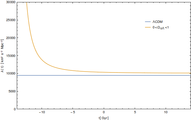
where and is the dimensionless parameter associated to the variable cosmological constant in the barotropic model. Thus, the number of free parameters in this case is reduced by one. The cosmic evolution of is given in Fig. 1 for the unique solution having phase transition in this model.33 3 The existence of future singularities induced by diffusion as shown in forthcoming sections implies that the redshift is not a monotonically decreasing function of time. Thus, hereon we use the cosmic time for the plots instead of the redshift.
In order to avoid negative energy density for matter fields, the condition must be met. This, in turn, implies
| (21) |
Since we have demanded for a reasonable scaling of the matter’s energy density, condition (21) implies that . This bound is saturated when , which is equivalent to demanding for .
Then, the Friedmann’s equations in a flat Universe for a matter dominated era are
| (22) | ||||
| (23) |
These equations admit exact solutions in four distinctive cases: (i) , (ii) , (iii) , and (iv) , which should be treated separately. In what follows, we define the parameter where, due to the previous considerations, implies that .
III.1.1 Case when
This case corresponds to a Universe filled only with a dark matter, whose energy density is modified by the factor introduced by [cf. Eq. (20)]. As we will see below, the solution for the scale factor resembles the one obtained for the Einstein–de Sitter model, i.e.
| (24) |
where is an integration constant. Since , this solution represents a power-law expansion without phase transition, and therefore is disfavored by observations. It can be decelerated or accelerated for if is lesser or greater than 1, respectively.
III.1.2 Case when
Since we have previously demanded , this case implies from Eq. (20). Thus, the evolution corresponds to a de Sitter solution with a scale factor
| (25) |
where is an integration constant and . We shall not consider this solution from now on.
III.1.3 Case when
In this scenario, dark matter coexists with negative pressure dark energy modeled by the variable cosmological constant . Since the dark matter density is a decreasing function of time, the variable cosmological constant also decreases as the cosmic time evolves, going to a constant value (see Fig. 2).44 4 A similar behavior is found for the CSL model of Sec. III.2, that has been previously outlined in Ref. Josset et al. 2017. Therefore, it is expected that a phase transition from a decelerated to accelerated expansion occurs, ending with a de Sitter-like behavior. In fact, the Friedmann’s equations in this case are solved by
| (26) |
Thus, it becomes clear that this solution possesses a phase transition and its behavior is more likely to describe the observational data. The age of the Universe in this case is
| (27) |
where the integration constant has been fixed according to the normalization . This solution will be taken into account in forthcoming sections to be constrained with cosmological data.

III.1.4 Case when
The last possibility characterizes a Universe filled with dark matter and a negative integration constant . This solution represents an anti-de Sitter Universe with future cosmological singularity, whose scale factor is given by
| (28) |
where, recall, . However, it does not exhibit a phase transition and it is therefore unsupported by experimental data.
In sum, the barotropic model develops energy diffusion through dark matter where, for positive values of , it implies a energy loss as evolves. Four different exact solutions are found, depending on the value of integration cosmological constant. From an observational viewpoint, the most interesting one appears when , since it has a phase transition. This solution will be contrasted with SNe Ia and observational Hubble data later.
In the next section, we consider the specific form of the diffusion function obtained in Ref. Josset et al. 2017 for the CSL model in a cosmological setup and solve the field equations analytically.
III.2 Continuous spontaneous localization
The CSL model Pearle 1976; Ghirardi et al. 1986; Pearle 1989; Ghirardi et al. 1990; Bassi and Ghirardi 2003 is one of the most studied and refined approaches to solve the measurement problem of quantum mechanics. It describes quantum-to-classical transitions through stochastic and nonlinear terms in the Schrödinger equation, that produce the quantum collapse of the wave function. Remarkably, the appearance of energy divergences in collapse models Ballentine 1991; Pearle and Squires 1996; Bassi et al. 2005 can be avoided by introducing energy dissipation of matter Smirne et al. 2014; Smirne and Bassi 2015, which has been shown to be compatible with the volume-preserving diffeomorphisms invariance of UG Josset et al. 2017.55 5 It is worth mentioning that an additional framework with similar predictions is the causal set approach to quantum gravity Dowker et al. 2004; Philpott et al. 2009. For concreteness, we restrict ourselves to the CSL setup and leave causal sets for a future studies. In this Subsection, we focus on this scenario that provides a specific prediction for the diffusion function .
For matter, the CSL model predicts a characteristic form of the diffusion function that can be expressed as Josset et al. 201766 6 In Ref. Josset et al. 2017, this form was taken for baryons only. Here, we consider that dark matter behaves similarly to baryons, although an extension that distinguishes their nature is straightforward.
| (29) |
where is an integration constant and is the energy density of the matter content. As we will see next, contributes to an effective value of the integration constant that plays the role of the cosmological constant. The latter will be fixed by initial data through their corresponding Friedmann’s constraint. Moreover, current experimental data impose severe constraints on the free parameter according to (see Josset et al. 2017 and references therein).
Assuming a dustlike dark matter component, the conservation law (13) is solved by
| (30) |
where is an integration constant related to the present energy density of matter. Thus, the effect of energy diffusion in the CSL model is to provide a modulation of the scaling of matter. Although one would expect an exponential grow of energy density at late times, the backreaction of diffusion generates a similar modification on the scale factor [see Eqs. (36)-(40) below] that cancels out the exponential in Eq. (30), producing a decay on the energy density as long as the scale factor grows.
Considering that only dark matter develops diffusion, the Friedmann’s equations in the CSL scenario become
| (31) | ||||
| (32) |
where and represents its value at present time. In the flat case, and defining the quantity (with denoting its present value), we find that these equations admit exact solutions in three distinct cases: (i) , (ii) , and (iii) .
The Friedmann’s constraints for each case are
| (33) | ||||
| (34) |
where the upper and lower signs of Eq. (33) correspond to the first and second cases, respectively, while Eq. (34) corresponds to the third case. To obtain a clearer meaning of Eqs. (33) and (34) before the analytical solutions are presented, we subtract in their both sides and take their second power. Both results can be summarized in
| (35) |
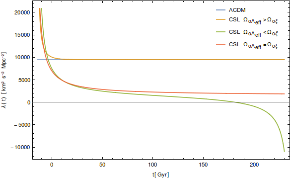
where is contained as a particular case. Thus, is interpreted as the dimensionless parameter associated to the variable cosmological constant for the CSL model. Remarkably, the case when [i.e. with the minus sign in Eq. (35)], admits a sign flip of the variable cosmological constant as time evolves, passing from a de Sitter to an anti de Sitter phase at very late times. Its cosmic evolution is displayed in Fig. 3 for the three analytical solutions found below.
In the following, we discuss each of these cases separately and provide the analytic form of the scale factor that solves Eqs. (31) and (32). Remarkably, it is found that the presence of energy diffusion generates an exponential modulation of the scale factor in all cases. This feature induces a phase transition from decelerated to accelerated expansion, providing a suitable setup to be constrained by cosmological data.
III.2.1 Case when
This scenario represents a Universe filled with dark matter, where the effective integration constant dominates over energy diffusion at present time. Therefore, in the constraint given by Eq. (35), the variable cosmological constant remains positive during the whole evolution. In fact, solving the Friedmann’s equations (31) and (32), we obtain a scale factor
| (36) |
Remarkably, this solution represents a Universe with phase transition from deceleration to acceleration driven by energy diffusion induced by quantum collapse, with a de Sitter-like expansion at late times. The age of the Universe in this scenario is
| (37) |
where the integration constant has been fixed by .
III.2.2 Case when
In this scenario, the Universe is filled with dark matter whose diffusion function dominates over the cosmological integration constant. The constraint given by Eq. (33) indicates that decreases to a minimum value and the variable cosmological constant takes negative values at late times (see Figs. 3 and 5). This behavior is encoded in the solution of the scale factor as a function of the cosmic time, i.e.,
| (38) |
Therefore, the exponential modulation induced by quantum collapse generates a phase transition during the period when the variable cosmological constant remains positive. As time evolves, it can take negative values, leading to a big crunch for very far future times. The behavior of the scale factor of this solution is plotted in Fig. 4, while the variable cosmological constant is included in Fig. 5. The age of the Universe in this case is given by
| (39) |
where, as before, the integration constant has been fixed according to .
III.2.3 Case when
Whenever the dimensionless parameters related to the effective integration constant and energy diffusion are equal at present time, the function goes to its minimum value as long as goes to zero with the cosmic expansion. Thus, the variable cosmological constant reaches a nontrivial asymptotic value and it is expected to have a de Sitter-like expansion at late times driven by . Integrating Eqs. (31) and (32) we obtain the scale factor, which takes the form
| (40) |
This solution represents a power-law expansion modulated by an exponential function of the cosmic time, with a de Sitter behavior at late times. Remarkably, it has a phase transition from decelerated to accelerated expansion due to the nontrivial contribution of energy diffusion. The age of the Universe in this case is
| (41) |
where the normalization has been used.


In the next section, we constrain the parameters of the barotropic and CSL models using observational data for a flat FLRW Universe. To this end, we focus on solutions possessing phase transition and compare them with observational Hubble data (OHD) and SNe Ia data.
IV Cosmological constraints
To impose the constraints on the preceding models, we compute the best-fit value of their parameters by means of the affine-invariant Markov Chain Monte Carlo method (MCMC) Goodman and Weare 2010. This is implemented in the pure-Python code emcee Foreman-Mackey et al. 2013 by setting 24 chains with 4500 steps. In order for the latter to explore the whole parameter space and get settled in the maximum of the probability density, 1500 burn-in steps are performed beforehand.
Since we are implementing Bayesian statistical analysis to estimate the free parameters and their confidence regions, we construct the Gaussian likelihood function
| (42) |
Here, is a normalization constant and stands for each data set under consideration, namely OHD, SNe Ia, and their joint analysis with . They are described in the following, alongside their functions.
IV.1 Observational Hubble Data
To constrain the models with OHD, we use the data set of Ref. Magaña et al. 2018 that consists of 51 Hubble data points in the redshift range . In this catalog, 31 data points are obtained by the differential age method Jimenez and Loeb 2002, where the points can be estimated using
| (43) |
with being measured using the break feature as a function of the redshift. This method is model independent since it relies on the metallicity and the age of the stellar population of early galaxies estimated through spectroscopy. The remaining data points come from measurements of baryon acoustic oscillation, assuming that the data of is obtained independently. Hence, the merit function of the OHD is constructed as
| (44) |
where and are the observational and theoretical Hubble parameters at redshift , respectively, is the associated error of , and denotes the free parameters.
It is worth mentioning that we consider the present value of the Hubble constant as a free parameter as well. Thus, for the Bayesian analysis, we use a Gaussian prior over the dimensionless Hubble parameter, , where and are the mean value and standard deviation, respectively. This is done according to , measured with a of uncertainty Riess et al. 2016.
IV.2 Type Ia Supernovae
In addition to OHD, SNe Ia data can be used to constrain the models. Currently, there are three main catalogs: Union 2.1 with 557 points in the redshift range Suzuki et al. 2012, JLA with 740 points in the redshift range Betoule et al. 2014, and Pantheon with 1048 point in the redshift range Scolnic et al. 2018. Here we focus on the latter that is a compilation of 279 SNe Ia data discovered by the Pan-STARRS1 Medium Deep Survey, combined with their estimated distance from the Sloan Digital Sky Survey, Supernova Legacy Survey, and various low- and Hubble Space Telescope samples. In this case, the merit function is constructed as
| (45) |
where and are the observational and theoretical distance modulus of each SNe Ia at redshift , respectively, is the error in the measurement of , and encompasses the free parameters of the respective model.
In the Pantheon sample, the observational distance modulus is obtained by using the modified version of the Tripp formula Tripp 1998. This method, however, is endowed with at least three nuisance parameters that must be jointly estimated with the cosmological parameters . To overcome this problem, the method BEAMS with bias correction was proposed Kessler and Scolnic 2017, in which its value reduces to
| (46) |
where is the apparent B-band magnitude of a fiducial SNe Ia and is a nuisance parameter. Even more, the Pantheon sample gives the corrected apparent magnitude directly. On the other hand, the theoretical distance modulus in a flat FLRW spacetime of a given model is defined through the relation
| (47) |
where , is the speed of light given in units of , and is the luminosity given by
| (48) |
Equation (45) can be written in matrix notation (denoted by bold symbols) according to
| (49) |
where is the total covariance matrix given by
| (50) |
and we have defined . The entries of the diagonal matrix denote the statistical uncertainties of for each redshift, while denotes the systematic uncertainties in the BEAMS with bias correction approach.77 7 The Pantheon data set is available online in the GitHub repository https://github.com/dscolnic/Pantheon. The corrected apparent magnitude for each SNe Ia together with their respective redshifts and errors are available in the document lcparam_full_long.txt. The full systematic uncertainties matrix is available in the document sys_full_long.txt. In order to reduce the number of free parameters and marginalize over , we define with being an auxiliary nuisance parameter and being defined below Eq. (47). Thus, Eq. (49) can be expanded as Lazkoz et al. 2005
| (51) |
where
| (52) | ||||
| (53) | ||||
| (54) |
with .
Minimizing Eq. (51) with respect to gives and it reduces to
| (55) |
Notice that this function depends only on the free parameters of the model. In fact, Eq. (49) provides the same information as Eq. (55), since the best-fit parameters minimize the merit function. Then, gives an indication of the goodness of fit: the smaller its value, the better is the fit.
V Results and discussion
The two models are contrasted with OHD and SNe Ia data through their corresponding Hubble parameters. For the barotropic model, we consider the solution (22) subject to the Friedmann’s constraint (20). Hence, their free parameters are . For we use the flat prior , for we use the Gaussian prior , and for an EoS-like flat prior .
For the CSL model, on the other hand, we take into account all the solutions with phase transition, subject to the constraint (35). Thus, the free parameters of the first two cases are , while for the last one we have . The same priors as for the barotropic model are used for and . For , we consider a flat prior derived from Eq. (33), where the region allowed by laboratory experiments is contained. In each case, the Hubble parameter as a function of the redshift is obtained numerically.
For further comparison, we obtain the best fit of the free parameters of the CDM model after the Friedmann’s constraint, i.e. , with a flat prior , using
| (56) |
It is worth mentioning that a parameter in the emcee code is modified to obtain a mean acceptance fraction between and for each model Foreman-Mackey et al. 2013. Their values are 7 for CDM, 5 for the barotropic model, and 4 for the CSL model.
Even though the value of characterizes the goodness of the fit, it does not take into account the number of free parameters. Thus, one could add more of them at will such that the likelihood gets minimized. To overcome this problem, we compare their goodness through two statistical indicators: the Akaike Information Criterion (AIC) Akaike 1974 and the Bayesian Information Criterion (BIC) Schwarz 1978, defined, respectively as
| AIC | (57) | |||
| BIC | (58) |
Here, represents the maximum value of the likelihood function calculated for the best-fit parameters, is the number of free parameters, and is the number of the data samples. Thereby, these indicators characterize the model according to the number of free parameters, where the most favored one minimize their AIC and BIC values. Since the latter depends on the logarithm of the total observational data, it gives a better smoking gun than AIC. Thus, a model possessing a higher value of BIC when compared to the other is considered as a criterion against it.
From the observational data of OHD, SNe Ia, and their joint analysis, we provide the best-fit values for the parameters of each model in Table 1, alongside their AIC and BIC indicators. In Figs. 6-10, we show the allowed regions of the parameter space for the CDM, barotropic, and CSL models, respectively.
The results of Table 1 indicate that, for the joint analysis, the barotropic model has lower than CDM, reproducing better the cosmological data of SNe Ia and OHD. However, since CDM has less free parameters, it gives a lower BIC. Thus, even though we found evidence that CDM is statistically preferred, the small difference between their indicators is not strong enough to be conclusive about which model is better. In this case, the age of the Universe obtained from Eq. (27) is .
On the other hand, the CSL model with also reproduces better the cosmological data than CDM, as it can be seen from the difference of their in the joint analysis. The CDM model, in contrast, is statistically preferred as one concludes from their BIC’s values. However, the best fit of is translated into
| (59) |
which is clearly incompatible with previous laboratory experiments (see Josset et al. 2017 and references therein). This is in agreement with the conclusions of Ref. Martin and Vennin 2020 whose results obtained from the CMB are also in tension with earlier data. Moreover, imposing a prior compatible with preexisting data yields to similar values for and when compared to CDM, differing only in their associated errors. This indicates that the CSL model tends to the latter when the value of . Nevertheless, the obtained value for is not a best fit in this case, since it does not maximize the probability within the restricted prior. The age of the Universe in this case is .
| Data | Best-fit values | Goodness of fit | |||||
| AIC | BIC | ||||||
| CDM Model | |||||||
| OHD | - | - | |||||
| SNe Ia | - | - | |||||
| Joint | - | - | |||||
| Barotropic Model | |||||||
| OHD | - | ||||||
| SNe Ia | - | ||||||
| Joint | - | ||||||
| CSL Model with | |||||||
| OHD | - | ||||||
| SNe Ia | - | ||||||
| Joint | - | ||||||
| CSL Model with | |||||||
| OHD | - | ||||||
| SNe Ia | - | ||||||
| Joint | - | ||||||
| CSL Model with | |||||||
| OHD | - | - | |||||
| SNe Ia | - | - | |||||
| Joint | - | - | |||||
The cases when and do not minimize neither the nor the BIC’s value in comparison with CDM. Indeed, although the latter case has less free parameters than the barotropic and CSL model with , the large value of its undermines the remaining statistical indicators. Even more, in both cases, the best-fit values of obtained from the joint analysis of OHD and SNe Ia data are ruled out by model-independent estimations Holanda et al. 2019. Thus, we conclude that these two cases are not well supported by cosmological observations.
VI Conclusions and further remarks
In this work, we address the issue of higher-order equations generated by energy diffusion in homogeneous and isotropic UG García-Aspeitia et al. 2019a; García-Aspeitia et al. 2019b, by assuming an EoS that relates the diffusion function with the energy density of matter. It is worth recalling that diffusion is compatible with UG by virtue of its restricted diffeomorphism invariance, induced by the presence of the nondynamical -form , whose value is constrained through the cosmic history through Eq. (12). We study a Universe filled with dark matter that develops energy diffusion and, to determine their observational viability, two models possessing such a feature are considered and contrasted with cosmological data.
First, we study a barotropic model that incorporates the phenomenon of diffusion to gain intuition. Although the cosmological integration constant is fixed by initial data, energy diffusion introduces an additional parameter. Four exact solutions are found in this scenario, with one of them having a phase transition from decelerated to accelerated expansion. Remarkably, this model is successful at describing the joint analysis of OHD and SNe Ia data, even though CDM is statistically preferred for having less free parameters. However, their small difference in BIC’s value indicates that, in order to be conclusive, more data are needed.
Second, a well-known scenario with energy-momentum nonconservation generated by quantum collapse is analyzed: the CSL model. Three analytical homogeneous and isotropic solutions are found. Remarkably, all of them possess phase transition induced by energy diffusion. When contrasted with observations, the CSL model with gives, according to experimental data, a better description of the cosmological evolution than CDM model. Nevertheless, the latter has fewer free parameters and it is therefore more favorable from a statistical viewpoint. However, the best-fit value of forces the free parameter of the CSL model to lie in a region that is incompatible with other laboratory experiments. On the other hand, the cases when and give neither a good fit nor a compatible prediction with model-independent measurements of .
Even though we found evidence that some cases studied here tend to CDM asymptotically, the source of the accelerated expansion is radically different in scenarios with diffusion. Interestingly enough, the CSL model that emulates a variable cosmological constant with sign flip at late times opens the possibility of having a Universe with phase transition from de Sitter to anti de Sitter expansion with a very far future cosmological singularity: a big crunch. The absence of turning points in the Hubble parameter, as predicted by CDM and supported by experiments, is a remarkable feature of the aforementioned models possessing a sign flip in the variable cosmological constant. This may be an attractive consequence regarding the swampland criteria on cosmology Agrawal et al. 2018. Although different scenarios with variable cosmological constant have been proposed beyond CDM Caldwell et al. 1998; Clifton et al. 2012; van Putten 2015; Ó Colgáin et al. 2019; van Putten 2019, diffusion provides a rich phenomenology dispensing from additional fields and higher-curvature corrections to the Einstein–Hilbert action.
It is worth mentioning that the constraints obtained here are model dependent. Indeed, we found that diffusion is not ruled out by SNe Ia or Hubble data in the barotropic model, providing an appealing approach to describe late-time acceleration. This may open new avenues to be explored, for instance, in the context of cosmological perturbations. In Ref. Gao et al. 2014, it was shown that UG could have observable effects in the CMB through the Sachs–Wolfe effect Sachs and Wolfe 1967. For adiabatic fluctuations, however, the differences with GR are negligible at large scales. Later, the same effect was computed in gauge-invariant way, concluding that cosmological perturbations of UG and GR are identical Basak et al. 2016. Nevertheless, both studies assumed the conservation of the energy-momentum tensor and it is certainly of great interest to study the effect of energy diffusion to determine whether it could affect the CMB or structure formation.
On the other hand, the only viable case of the CSL model, namely , is in tension with previous constraints, since the best-fit values of in Eq. (59) are incompatible with Toroš et al. 2017 (see also Josset et al. 2017). The nature of this incompatibility is different from Ref. Martin and Vennin 2020, whose limitations in the inflationary epoch were recently pointed out in Bengochea et al. 2020. The extrapolation in this work is far less dramatic than Martin and Vennin 2020, since the effects of diffusion start from hadronization to the present time. Of course, there is still the possibility that the effective parameters changed after nucleosynthesis, affecting the estimations done here. This fact reinforces the idea of keep exploring the implications of energy diffusion in cosmology, in particular collapse models.
An appealing approach to restore the energy-momentum conservation in UG is to consider interacting fluids. Although their energy-momentum tensor may not need to be conserved individually, their interaction could imply a energy conservation of the whole system.88 8 We thank A. Arza for pointing this out. This setup has been considered in different scenarios Chimento 2006; Cataldo et al. 2008; Farajollahi et al. 2010; Lip 2011; Cotsakis and Kittou 2012; Elizalde and Khurshudyan 2017; Cruz et al. 2019, but it has not been implemented in UG. The cosmological consequences of such interaction are worth exploring, since the backreaction of more than one fluid becomes relevant in phase transitions between different matter dominated eras. The predictions of the interacting model can be contrasted with observational data in the same spirit as it has been done here. These studies are relevant for determining the viability of UG with energy-momentum nonconservation and they are left for future contributions.
Acknowledgements.
The authors thank to Ariel Arza, Yuri Bonder, Eoin Ó. Colgáin, Daniel Sudarsky, Maurice H.P.M. van Putten, and Nelson Videla for valuable comments. C.C. thanks the hospitality of Universidad de Santiago de Chile as well as the partial support of Proyecto POSTDOC_DICYT, Código 041931CM_POSTDOC, Universidad de Santiago de Chile. N.C. is partially supported by the Dirección de Investigación Científica y Tecnológica (Dicyt) from Universidad de Santiago de Chile through Grant N∘ 041831CM.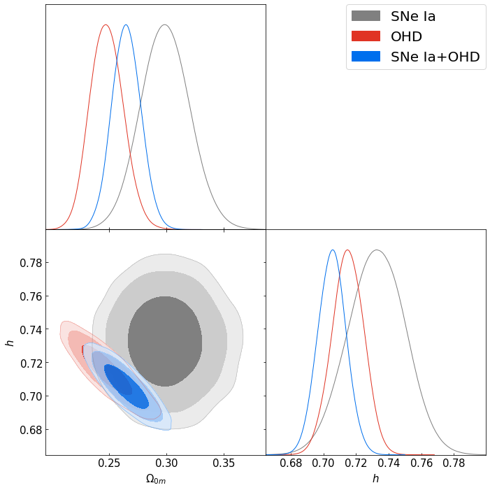


References
- Riess et al. (1998) A. G. Riess et al., Astron. J. 116, 1009 (1998).
- Perlmutter et al. (1999) S. Perlmutter et al., Astrophys. J. 517, 565 (1999).
- Hinshaw et al. (2013) G. Hinshaw et al., Astrophys. J. Suppl. Ser. 208, 19 (2013).
- Ade et al. (2016) P. A. R. Ade et al. (Planck), Astron. Astrophys. 594, A13 (2016).
- Moresco et al. (2016) M. Moresco, L. Pozzetti, A. Cimatti, R. Jimenez, C. Maraston, L. Verde, D. Thomas, A. Citro, R. Tojeiro, and D. Wilkinson, JCAP 1605, 014 (2016).
- Weinberg (1989) S. Weinberg, Rev. Mod. Phys. 61, 1 (1989).
- Addison et al. (2018) G. E. Addison, D. J. Watts, C. L. Bennett, M. Halpern, G. Hinshaw, and J. L. Weiland, Astrophys. J. 853, 119 (2018).
- Macaulay et al. (2019) E. Macaulay et al. (DES), Mon. Not. Roy. Astron. Soc. 486, 2184 (2019).
- Wong et al. (2019) K. C. Wong et al., (2019), arXiv:1907.04869 [astro-ph.CO] .
- Riess et al. (2016) A. G. Riess et al., Astrophys. J. 826, 56 (2016).
- Riess et al. (2018) A. G. Riess et al., Astrophys. J. 861, 126 (2018).
- Riess et al. (2019) A. G. Riess, S. Casertano, W. Yuan, L. M. Macri, and D. Scolnic, Astrophys. J. 876, 85 (2019).
- (13) N. Aghanim et al. (Planck), arXiv:1807.06209 [astro-ph.CO] .
- Bennett et al. (2014) C. L. Bennett, D. Larson, J. L. Weiland, and G. Hinshaw, Astrophys. J. 794, 135 (2014).
- Cardona et al. (2017) W. Cardona, M. Kunz, and V. Pettorino, JCAP 1703, 056 (2017).
- Feeney et al. (2018) S. M. Feeney, D. J. Mortlock, and N. Dalmasso, Mon. Not. Roy. Astron. Soc. 476, 3861 (2018).
- Zhang et al. (2017) B. R. Zhang, M. J. Childress, T. M. Davis, N. V. Karpenka, C. Lidman, B. P. Schmidt, and M. Smith, Mon. Not. Roy. Astron. Soc. 471, 2254 (2017).
- Einstein (1919) A. Einstein, Sitzungsber. Preuss. Akad. Wiss. Berlin (Math. Phys.) 1919, 349 (1919).
- Anderson and Finkelstein (1971) J. L. Anderson and D. Finkelstein, Am. J. Phys. 39, 901 (1971).
- van der Bij et al. (1982) J. J. van der Bij, H. van Dam, and Y. J. Ng, Physica 116A, 307 (1982).
- Buchmuller and Dragon (1988) W. Buchmuller and N. Dragon, Phys. Lett. B 207, 292 (1988).
- Unruh (1989) W. G. Unruh, Phys. Rev. D 40, 1048 (1989).
- Henneaux and Teitelboim (1989) M. Henneaux and C. Teitelboim, Phys. Lett. B 222, 195 (1989).
- Ng and van Dam (1991) Y. J. Ng and H. van Dam, J. Math. Phys. 32, 1337 (1991).
- Finkelstein et al. (2001) D. R. Finkelstein, A. A. Galiautdinov, and J. E. Baugh, J. Math. Phys. 42, 340 (2001).
- Ellis et al. (2011) G. F. R. Ellis, H. van Elst, J. Murugan, and J.-P. Uzan, Class. Quant. Grav. 28, 225007 (2011).
- Álvarez (2005) E. Álvarez, JHEP 03, 002 (2005).
- Álvarez et al. (2006) E. Álvarez, D. Blas, J. Garriga, and E. Verdaguer, Nucl. Phys. B756, 148 (2006).
- Jain et al. (2012) P. Jain, A. Jaiswal, P. Karmakar, G. Kashyap, and N. K. Singh, JCAP 1211, 003 (2012).
- Barvinsky and Kamenshchik (2017) A. O. Barvinsky and A. Yu. Kamenshchik, Phys. Lett. B774, 59 (2017).
- Álvarez et al. (2008) E. Álvarez, A. F. Faedo, and J. J. Lopez-Villarejo, JHEP 10, 023 (2008).
- Smolin (2009) L. Smolin, Phys. Rev. D80, 084003 (2009).
- Fiol and Garriga (2010) B. Fiol and J. Garriga, JCAP 1008, 015 (2010).
- Barceló et al. (2014) C. Barceló, R. Carballo-Rubio, and L. J. Garay, Phys. Rev. D89, 124019 (2014).
- Padilla and Saltas (2015) A. Padilla and I. D. Saltas, Eur. Phys. J. C75, 561 (2015).
- Saltas (2014) I. D. Saltas, Phys. Rev. D90, 124052 (2014).
- Álvarez et al. (2015a) E. Álvarez, S. González-Martín, M. Herrero-Valea, and C. P. Martín, Phys. Rev. D92, 061502 (2015a).
- Álvarez et al. (2015b) E. Álvarez, S. González-Martín, M. Herrero-Valea, and C. P. Martín, JHEP 08, 078 (2015b).
- Bufalo et al. (2015) R. Bufalo, M. Oksanen, and A. Tureanu, Eur. Phys. J. C75, 477 (2015).
- Eichhorn (2015) A. Eichhorn, JHEP 04, 096 (2015).
- Benedetti (2016) D. Benedetti, Gen. Rel. Grav. 48, 68 (2016).
- Josset et al. (2017) T. Josset, A. Perez, and D. Sudarsky, Phys. Rev. Lett. 118, 021102 (2017).
- de León Ardón et al. (2018) R. de León Ardón, N. Ohta, and R. Percacci, Phys. Rev. D97, 026007 (2018).
- Percacci (2018) R. Percacci, Found. Phys. 48, 1364 (2018).
- Jirouˇsek and Vikman (2019) P. Jirouˇsek and A. Vikman, JCAP 04, 004 (2019).
- Hammer et al. (2020) K. Hammer, P. Jirousek, and A. Vikman, (2020), arXiv:2001.03169 [gr-qc] .
- Nojiri et al. (2016) S. Nojiri, S. D. Odintsov, and V. K. Oikonomou, JCAP 1605, 046 (2016).
- Bamba et al. (2017) K. Bamba, S. D. Odintsov, and E. N. Saridakis, Mod. Phys. Lett. A32, 1750114 (2017).
- Nassur et al. (2016) S. B. Nassur, C. Ainamon, M. J. S. Houndjo, and J. Tossa, Eur. Phys. J. Plus 131, 420 (2016).
- Rajabi and Nozari (2017) F. Rajabi and K. Nozari, Phys. Rev. D96, 084061 (2017).
- Houndjo (2017) M. J. S. Houndjo, Eur. Phys. J. C77, 607 (2017).
- Álvarez and González-Martín (2015) E. Álvarez and S. González-Martín, Phys. Rev. D92, 024036 (2015).
- Bonder and Corral (2018) Y. Bonder and C. Corral, Phys. Rev. D97, 084001 (2018).
- Anero et al. (2020a) J. Anero, C. P. Martin, and R. Santos-Garcia, JHEP 01, 145 (2020a).
- Anero et al. (2020b) J. Anero, C. P. Martin, and R. Santos-Garcia, (2020b), arXiv:2001.05365 [hep-th] .
- Perez and Sudarsky (2019a) A. Perez and D. Sudarsky, Phys. Rev. Lett. 122, 221302 (2019a).
- Perez et al. (2018) A. Perez, D. Sudarsky, and J. D. Bjorken, Int. J. Mod. Phys. D27, 1846002 (2018).
- Kossakowski (1972) A. Kossakowski, Rep. Math. Phys. 3, 247 (1972).
- Lindblad (1976) G. Lindblad, Commun. Math. Phys. 48, 119 (1976).
- Banks et al. (1984) T. Banks, L. Susskind, and M. E. Peskin, Nucl. Phys. B244, 125 (1984).
- Unruh and Wald (1995) W. G. Unruh and R. M. Wald, Phys. Rev. D52, 2176 (1995).
- Hawking (1976) S. W. Hawking, Phys. Rev. D14, 2460 (1976).
- Perez et al. (2020) A. Perez, D. Sudarsky, and E. Wilson-Ewing, (2020), arXiv:2001.07536 [astro-ph.CO] .
- Perez and Sudarsky (2019b) A. Perez and D. Sudarsky, (2019b), arXiv:1911.06059 [gr-qc] .
- Astorga-Moreno et al. (2019) J. A. Astorga-Moreno, J. Chagoya, J. C. Flores-Urbina, and M. A. Garcia-Aspeitia, JCAP 1909, 005 (2019).
- Alho and Calogero (2017) A. Alho and S. Calogero, J. Geom. Phys. 120, 62 (2017).
- Calogero (2012) S. Calogero, J. Geom. Phys. 62, 2208 (2012).
- Calogero and Velten (2013) S. Calogero and H. Velten, JCAP 11, 025 (2013).
- Benisty and Guendelman (2017) D. Benisty and E. Guendelman, Eur. Phys. J. C 77, 396 (2017).
- Benisty and Guendelman (2018) D. Benisty and E. I. Guendelman, Int. J. Mod. Phys. A 33, 1850119 (2018).
- Benisty et al. (2019) D. Benisty, E. Guendelman, and Z. Haba, Phys. Rev. D 99, 123521 (2019), [Erratum: Phys. Rev. D101, 049901 (2020)].
- Daouda et al. (2019) M. Daouda, J. Fabris, A. Oliveira, F. Smirnov, and H. Velten, Int. J. Mod. Phys. D 28, 1950175 (2019).
- García-Aspeitia et al. (2019a) M. A. García-Aspeitia, C. Martínez-Robles, A. Hernández-Almada, J. Magaña, and V. Motta, Phys. Rev. D99, 123525 (2019a).
- García-Aspeitia et al. (2019b) M. A. García-Aspeitia, A. Hernández-Almada, J. Magaña, and V. Motta, (2019b), arXiv:1912.07500 .
- Weinberg (2008) S. Weinberg, Cosmology (2008).
- Pearle (1976) P. M. Pearle, Phys. Rev. D13, 857 (1976).
- Ghirardi et al. (1986) G. C. Ghirardi, A. Rimini, and T. Weber, Phys. Rev. D34, 470 (1986).
- Pearle (1989) P. M. Pearle, Phys. Rev. A39, 2277 (1989).
- Ghirardi et al. (1990) G. C. Ghirardi, P. M. Pearle, and A. Rimini, Phys. Rev. A42, 78 (1990).
- Martin and Vennin (2020) J. Martin and V. Vennin, Phys. Rev. Lett. 124, 080402 (2020).
- Bassi and Ghirardi (2003) A. Bassi and G. C. Ghirardi, Phys. Rept. 379, 257 (2003).
- Ballentine (1991) L. E. Ballentine, Phys. Rev. A 43, 9 (1991).
- Pearle and Squires (1996) P. M. Pearle and E. Squires, Found. Phys. 26, 291 (1996).
- Bassi et al. (2005) A. Bassi, E. Ippoliti, and B. Vacchini, Journal of Physics A: Mathematical and General 38, 8017 (2005).
- Smirne et al. (2014) A. Smirne, B. Vacchini, and A. Bassi, Phys. Rev. A 90, 062135 (2014).
- Smirne and Bassi (2015) A. Smirne and A. Bassi, Scientific Reports 5, 12518 (2015).
- Dowker et al. (2004) F. Dowker, J. Henson, and R. D. Sorkin, Mod. Phys. Lett. A19, 1829 (2004).
- Philpott et al. (2009) L. Philpott, F. Dowker, and R. D. Sorkin, Phys. Rev. D79, 124047 (2009).
- Goodman and Weare (2010) J. Goodman and J. Weare, Commun. Appl. Math. Comput. Sci. 5, 65 (2010).
- Foreman-Mackey et al. (2013) D. Foreman-Mackey, A. Conley, W. Meierjurgen Farr, D. W. Hogg, D. Lang, P. Marshall, A. Price-Whelan, J. Sanders, and J. Zuntz, Publ. Astron. Soc. Pac. 125, 306 (2013).
- Magaña et al. (2018) J. Magaña, M. H. Amante, M. A. Garcia-Aspeitia, and V. Motta, Mon. Not. Roy. Astron. Soc. 476, 1036 (2018).
- Jimenez and Loeb (2002) R. Jimenez and A. Loeb, Astrophys. J. 573, 37 (2002).
- Riess et al. (2016) A. G. Riess et al., Astrophys. J. 826, 56 (2016).
- Suzuki et al. (2012) N. Suzuki et al., Astrophys. J. 746, 85 (2012).
- Betoule et al. (2014) M. Betoule et al., Astron. Astrophys. 568, A22 (2014).
- Scolnic et al. (2018) D. M. Scolnic et al., Astrophys. J. 859, 101 (2018).
- Tripp (1998) R. Tripp, Astron. Astrophys. 331, 815 (1998).
- Kessler and Scolnic (2017) R. Kessler and D. Scolnic, Astrophys. J. 836, 56 (2017).
- Lazkoz et al. (2005) R. Lazkoz, S. Nesseris, and L. Perivolaropoulos, JCAP 2005, 010 (2005).
- Akaike (1974) H. Akaike, IEEE Transactions on Automatic Control 19, 716 (1974).
- Schwarz (1978) G. Schwarz, Annals of Statistics 6, 461 (1978).
- Holanda et al. (2019) R. Holanda, R. Gonçalves, J. Gonzalez, and J. Alcaniz, Journal of Cosmology and Astroparticle Physics 2019, 032 (2019).
- Agrawal et al. (2018) P. Agrawal, G. Obied, P. J. Steinhardt, and C. Vafa, Phys. Lett. B 784, 271 (2018).
- Caldwell et al. (1998) R. Caldwell, R. Dave, and P. J. Steinhardt, Phys. Rev. Lett. 80, 1582 (1998).
- Clifton et al. (2012) T. Clifton, P. G. Ferreira, A. Padilla, and C. Skordis, Phys. Rept. 513, 1 (2012).
- van Putten (2015) M. H. van Putten, Mon. Not. Roy. Astron. Soc. 450, L48 (2015).
- Ó Colgáin et al. (2019) E. Ó Colgáin, M. H. van Putten, and H. Yavartanoo, Phys. Lett. B 793, 126 (2019).
- van Putten (2019) M. H. P. M. van Putten, Monthly Notices of the Royal Astronomical Society: Letters 491, L6 (2019).
- Gao et al. (2014) C. Gao, R. H. Brandenberger, Y. Cai, and P. Chen, JCAP 1409, 021 (2014).
- Sachs and Wolfe (1967) R. K. Sachs and A. M. Wolfe, Astrophys. J. 147, 73 (1967).
- Basak et al. (2016) A. Basak, O. Fabre, and S. Shankaranarayanan, Gen. Rel. Grav. 48, 123 (2016).
- Toroš et al. (2017) M. Toroš, G. Gasbarri, and A. Bassi, Physics Letters A 381, 3921 (2017).
- Bengochea et al. (2020) G. R. Bengochea, G. Leon, P. Pearle, and D. Sudarsky, (2020), arXiv:2006.05313 [gr-qc] .
- Chimento (2006) L. P. Chimento, Phys. Lett. B633, 9 (2006).
- Cataldo et al. (2008) M. Cataldo, P. Mella, P. Minning, and J. Saavedra, Phys. Lett. B662, 314 (2008).
- Farajollahi et al. (2010) H. Farajollahi, N. Mohamadi, and H. Amiri, Mod. Phys. Lett. A25, 2579 (2010).
- Lip (2011) S. Z. W. Lip, Phys. Rev. D83, 023528 (2011).
- Cotsakis and Kittou (2012) S. Cotsakis and G. Kittou, Phys. Lett. B712, 16 (2012).
- Elizalde and Khurshudyan (2017) E. Elizalde and M. Khurshudyan, Int. J. Mod. Phys. D27, 1850037 (2017).
- Cruz et al. (2019) M. Cruz, S. Lepe, and G. Morales-Navarrete, Nucl. Phys. B 943, 114623 (2019).