Towards Exascale Lattice Boltzmann computing
Abstract
We discuss the state of art of Lattice Boltzmann (LB) computing, with special focus on prospective LB schemes capable of meeting the forthcoming Exascale challenge. After reviewing the basic notions of LB computing, we discuss current techniques to improve the performance of LB codes on parallel machines and illustrate selected leading-edge applications in the Petascale range. Finally, we put forward a few ideas on how to improve the communication/computation overlap in current large-scale LB simulations, as well as possible strategies towards fault-tolerant LB schemes.
1 Introduction
Exascale computing refers to computing systems capable of delivering Exaflops, one billion billions (, also known as quintillion) floating-point operations per second, that is one floating-point operation every billionth of a billionth of second, also known as Attosecond ( s).
Just to convey the idea, at Attosecond resolution, one can take a thousand snapshots of
an electron migrating from one atom to another to establish a new chemical bond.
Interestingly, the attosecond is also the frontier of current day atomic clock precision, which means clocks that lose or gain less than two seconds over the entire age of the Universe!
In 2009 Exascale was projected to occur in 2018, a prediction which turned out to be fulfilled just months ago,
with the announcement of a 999 PF/s sustained throughput computational using the SUMMIT supercomputer [1]11
1
This figure was obtained using half precision (FP16) floating point arithmetic..
Mind-boggling as they are, what do these numbers imply for the actual advancement of science?
The typical list includes new fancy materials, direct simulation of biological organs, fully-digital design of cars and airplanes with no need of building physical prototypes, a major boost in cancer research, to name but a few.
Attaining Exaflop performance on each of these applications, however, is still an open challenge,
because it requires a virtually perfect match between the system architecture and
the algorithmic formulation of the mathematical problem.
In this article, we shall address the above issues with specific reference to a class of mathematical
models known as Lattice Boltzmann (LB) methods, namely a lattice formulation of Boltzmann’s kinetic equation
which has found widespread use across a broad range of problems involving complex states of flowing
matter [2].
The article is organized as follows: in Section 2 we briefly introduce the basic features of the LB method.
In Section 3 the state of-the-art of LB performance implementation will be briefly presented,
whereas in Section 4 the main aspects of future exascale computing are discussed,
along with performance figures for current LB schemes on present-day Petascale machines.
Finally, in Section 5 we sketch out a few tentative ideas which may facilitate the migration of LB
codes to Exascale platforms.
2 Basic Lattice Boltzmann Method
The LB method was developed in the late 1980’s as a noise-free replacement of lattice gas cellular automata
for fluid dynamic simulations [2].
Ever since, it has featured a (literal) exponential growth of applications across
a remarkably broad spectrum of complex flow problems, from fully developed turbulence
to micro and nanofluidics [3], all the way down to quark-gluon plasmas [4, 5].
The main idea is to solve a minimal Boltzmann kinetic equation for a set
of discrete distribution functions (populations in LB jargon) , expressing
the probability of finding a particle at position and time , with a (discrete) velocity .
The set of discrete velocities must be chosen in such a way as to secure enough symmetry
to comply with mass-momentum-energy conservation laws of macroscopic hydrodynamics, as well as
with rotational symmetry.
Figure 1 shows two of the 3D lattices most widely used for current LB simulations, with a set of 19 discrete velocities (D3Q19) or 27 velocities (D3Q27).
In its simplest and most compact form, the LB equation reads as follows:
| (1) |
where and are 3D vectors in ordinary space, is the equilibrium distribution function
and the lattice time step is made unit, so that is the length of the link connecting a generic lattice site
node to its neighbors, .
In the above, the local equilibria are provided by a lattice truncation, to
second order in the Mach number , of the Maxwell-Boltzmann distribution, namely
| (2) |
where is a set of weights normalized to unity,
and , in spatial dimensions.
Finally, is a source term encoding the fluid interaction with external (or internal) sources, the latter
being crucial to describe multiphase flows with potential energy interactions.
The above equation represents the following situation: the populations at site at time
collide to produce a post-collisional state , which is then scattered away
to the corresponding neighbors at at time .
Provided the lattice is endowed with suitable symmetries, and the local equilibria
are chosen accordingly, the above scheme can be shown to reproduce the
Navier-Stokes equations for an isothermal quasi-incompressible fluid of density and velocity
| (3) |
The relaxation parameter dictates the viscosity of the lattice fluid according to
| (4) |
Full details can be found in the vast literature on the subject [6][7].
2.1 The stream-collide LB paradigm
The main strength of the LB scheme is the stream-collide paradigm, which stands
in marked contrast with the advection-diffusion of the macroscopic
representation of fluid flows.
Unlike advection, streaming proceeds along straight lines defined by the discrete
velocities , regardless of the complexity of the fluid flow.
This is a major advantage over material transport
taking place along fluid lines, whose tangent is given by the fluid velocity itself, a highly
dynamic and heterogeneous field in most complex flows.
To be noted that streaming is literally exact. i.e., there is no round-off error, as it
implies a memory shift only with no floating-point operation.
For the case of a 2D lattice, discounting boundary conditions, the streaming along positive
and negative (p=1, 2) can be coded as shown in Algorithms 2.1 and 2.1.
Note that the second loop runs against the flow, i.e. counterstream, so as to avoid overwriting
memory locations, which would result in advancing the same population across the
entire lattice in a single time step!
A similar trick applies to all other populations: the loops
must run counter the direction of propagation.
This choice makes possible to work with just a single array for time levels and , thereby halving the memory requirements.
With this streaming in place, one computes the local equilibria distribution as a
quadratic combination of the populations and moves on to the collision step, as shown in pseudocode 2.1.
This completes the inner computational engine of LB.
In this paper, we shall not deal with boundary conditions, even though, like with any
computational fluid-dynamic method, they ultimately decide the quality of the simulation results.
We highlight only that the exact streaming permits to handle fairly complex
boundary conditions in a conceptually transparent way [9] because information always moves along the straight lines defined by the discrete velocities.
Actual programming can be laborious, though.
———————————————————————————————
Algorithm 2.1: In-place streaming (.)
———————————————————————————————
Algorithm 2.2: In-place streaming (.)
———————————————————————————————
Algorithm 2.3: Collision step(.)
3 Improving LB performance
The LB literature provides several “tricks” to accelerate the execution of the basic LB algorithms above described. Here we shall briefly describe three major ones, related to optimal data storage and access, as well as parallel performance optimisation.
3.1 Data storage and allocation
The Stream-Collide paradigm is very powerful, but due to the comparatively large number
of discrete velocities, it shows exposure to memory bandwidth issues, i.e. the number
of bytes to be moved to advance the state of each lattice site from time to .
Such data access issues have always been high on the agenda of efficient LB implementations,
but with prospective Exascale LB computing in mind, they become vital.
Thus, one must focus on efficient data allocation and access practices.
There are two main and mutually conflicting ways of storing LB populations (assuming row-major memory order as in
C or C++ languages):
- •
By contiguously storing the set of populations living in the same lattice site:
fpop[nx][ny][npop](AoS, Array of Structures) - •
By contiguously storing homologue streamers across the lattice:
fpop[npop][nx][ny](SoA, Structure of Arrays)
The former scenario, AoS, is optimal for collisions since the collision
step requires no information from neighbouring populations and it is also
cache-friendly, as it presents unit stride access, i.e., memory
locations are accessed contiguously, with no jumps in-between.
However, AoS is non-optimal for streaming, whose stride is now equal
to npop, the number of populations.
The latter scenario, SoA, is just reciprocal, i.e., optimal for streaming, since it features a unitary stride, but
inefficient for collisions, because it requires npop different streams of data at the same time.
These issues are only going to get worse as more demanding applications
are faced, such multiphase or multicomponent flows requiring more populations
per lattice site and often also denser stencils.
Whence the need of developing new strategies for optimal data storage and access.
A reliable performance estimate is not simple, as it depends on a number of hardware platform parameters, primarily
the latency and bandwidth of the different levels of memory hierarchy.
An interesting strategy has been presented by Aniruddha and coworkers [11],
who proposed a compromising data organization, called AoSoA.
Instead of storing all populations on site, they propose to store only relevant
subsets, namely the populations sharing the same energy (energy-shell organization).
For instance, for the D3Q27 lattice, this would amount to four energy shells:
energy (just 1 population), energy (6 populations),
energy (12 populations) and energy (8 populations).
This is sub-optimal for collisions but relieves much strain from streaming.
As a matter of fact, by further ingenuous sub-partitioning of the energy shells, the authors manage to capture the best of the two, resulting in an execution of both Collision and Streaming
at their quasi-optimal performance.
Note that in large-scale applications, streaming can take up to per cent of the execution time
even though it does not involve any floating-point operation!
In [10] a thorough analysis of various data allocation policies is presented.
3.2 Fusing Stream-Collide
Memory access may take a significant toll if stream and collide are kept as separate steps (routines).
Indeed, node-wise, using a single-phase double precision D3Q19 LB scheme, there are
bytes involved in memory operations (load/store) per
Flops of computation, corresponding to a rough computation to memory ratio of Flops/Byte.
The memory access issue was recognized since the early days of
LB implementations and led to the so-called fused, or push, scheme.
In the fused scheme (eq. 5), streaming is, so to say, “eaten up” by collisions
and replaced by non-local collisions [12].
| (5) |
where is the pointee of site along the -th direction.
As one can appreciate, the streaming has virtually disappeared, to be
embedded within non-local collisions, at the price of doubling memory requirements (two separate arrays at and are needed) and a more complex load/store operation.
Actually, fused versions with a single memory level have also appeared in the literature,
but it is not clear whether their benefits are worth the major programming complications they entail [13].
Moreover the chance of executing them in parallel mode is much more limited.
3.3 Hiding communication costs
The third major item, which is absolutely crucial for multiscale applications, where
LB is coupled to various forms of particle methods, is the capability of hiding the
communication costs by overlapping communication and calculation when running in parallel mode.
Technically, this is achieved by using non-blocking communication
send/receive MPI primitives as shown in pseudo-algorithm 3.3:
———————————————————————————————
Algorithm 3.1: non-blocking Receive(.)
where is the boundary data to be transferred from source to destination, in order
for the latter to perform its chunk of computation.
The send operation is usually non-blocking, i.e. the source task keeps doing other
work while the memory sub-system is transmitting the data, because these data are, so to say, not its concern.
The destination task, on the other hand, cannot start the calculation until
those data are received, hence the safe procedure is to sit idle
until those data are actually received, i.e. the blocking-receive scenario.
However, if other work, not contingent to the reception of those data is
available, there is obviously no point of waiting, whence the point of non-blocking receive.
In other words, after posting its request for data from another task, the given
task proceeds with the calculations which are free from causal dependencies on the
requested data, until it is notified that these data are finally available.
This is of course way more complicated than just sitting idle until the requested data
arrive, as it requires a detailed command at the concurrent timeline of the parallel code.
However, non-blocking receive operations are absolutely key: without hiding communication costs, multiscale LB
applications would not get any near to the extreme performance they have attained in the last decade.
As an example, the multiscale code MUPHY [14]
scaled from tens of Teraflops in 2011 to 20 Petaflops in 2013, providing a precious
asset for the design of future exascale LB code.
A description of the state of the art of HPC LB can be found in [15].
4 Petascale and the roadmap to Exascale computers
Back in 1975, Gordon Moore predicted doubling of computing power every 18 months, namely
a thousandfold increase every fifteen years [16].
A unique case in the history of technology, such
prediction, now going by the name of Moore’s law, has proved correct
for the last four decades, taking from CRAY’s Megaflops of the early 80’s
to the current two hundreds Petaflops of Summit supercomputer [17].
Besides decreasing single-processor clock time, crucial to this achievement
has proven the ability of supercomputer architectures to support concurrent
execution of multiple tasks in parallel.
The current leading entries in the list of top-500 performers support up to
millions of such concurrent tasks and each CPU hosts tens of basic computing units, known as “cores”.
The promised 2020’s Exascale machine will cater to hundreds of
million of cores, with a core-clock still in the GHz range, because of heat power constraints.
As a consequence, an Exascale code should be prepared to exploit up to a billion concurrent
cores, each of them able to perform billions of floating point operations: .
This “symmetry” between computation and number of units that need to communicate
reflects and mandates a perfect balance between the two.
Indeed, as performance ramps up, it is increasingly apparent that accessing
data could become more expensive than make computations using them:
Bytes/s is taking over Flops/s as a metrics for extreme performance.
Besides hardware issues, Exascale computing also bears far-reaching implications on computational science, setting a strong premium on algorithms
with low data traffic, low I/O, lean communication to computation ratios and high fault-tolerance.
The point is simple, but worth a few additional comments.
Let being the number of Flops required by a given application, the corresponding number of Bytes,
the processing speed (Flops/s) and (Bytes/s) the corresponding bandwidth.
On the assumption of no overlap between memory access and computation, the execution time
is given by the sum of the two, namely:
| (6) |
The corresponding effective processing rate is given by:
| (7) |
where
| (8) |
This shows that in order to attain the peak performance , corresponding to
no data access overheads (infinite bandwidth), one must secure the condition .
Indeed, for , i.e., a “large” , we have , whereas in the opposite limit
, a “small” , the effective processing rate flattens at , i.e.,
a fraction of the bandwidth.
This is a (simplified) version of the so-called roofline model [18].
In a symbolic form, the roofline condition (8) can be written as
“Flops/Bytes much larger than (Flops/s)/(Bytes/s)”.
The former depends solely on the application, whereas the
latter is dictated by the hardware instead.
The “threshold” value, at which the transition between memory-bound to
floating-point-bound regimes occurs, is, for present hardware (fig. 2), .
4.1 Vanilla LB: back of envelope calculations
Using a simple Vanilla LB (VLB), i.e. single-phase, single time relaxation, 3D lattice with fused collision,
the roofline model permits to estimate limiting figures of performance. In Fig. 2 the roofline for an Intel phi is shown22
2
Bandwidth and Float point computation limits are obtained performing stream e HPL benchmark.
The technical name of the ratio between flops and data that need to be loaded/stored from/to memory is
Operational Intensity, OI for short, but we prefer to stick to our notation to keep
communication costs in explicit sight.
It provides information about code limitations: whether it is bandwidth-bound
() or floating-point bound (), as shown in Fig. 2.
The HPL code used to rank supercomputers [17] is floating-point bound
33
3
All hardware is built to exploit performance for floating point bound codes..
For a VLB, is the number of floating point operations per lattice site and time step
and is load/store demand in bytes, using double precision, hence
, which spells “bandwidth-bound”.
Boundary conditions operations are not considered here, for the sake of simplicity.
Memory Bandwidth in current-day hardware, at single node level, is about GB/s for an Intel Xeon Phi 7250 using MCDRAM in flat mode. MCDRAM is faster than RAM memory but it is limited in size ( GB). It can be used as a further cache level (cache mode) or auxiliary memory (flat mode) [19].
For a “standard server” like Intel Xeon Platinum 8160 server Memory Bandwidth is GB/s.
According to technological trends, bandwidth is not expected to exceed 500 GB/s by 2020 [20].
Using as LB performance metrics GLUPS (Giga Lattice Update Per Second), due to the fact that LB is memory bounded the peak value is 400 GB/s, the limit is yielding GLUPS for a Phi node, so that the
ratio , yielding an overhead factor : the effective processing speed is .
For an Exascale machine with order of nodes and GB/s Bandwidth per node, a peak of LUPS is expected.
4.2 Present-day Petascale LB application
As a concrete example of current-day competitive LB performance, we discuss the case of the
flow around a cylinder (Fig. 3, 4): the goal is to study the effect on vorticity
reduction using decorated cylinders [21] .
To describe short-scale decorations, such as those found in nature, resolutions in the Exascale range are demanded since the simulation can easily entail six spatial decades (meters to microns).
Clearly, more sophisticated techniques, such as grid-refinement [22], or unstructured
grids, could significantly reduce the computational demand, but we shall not delve into these matters here.
Indeed, if the “simple” computational kernel is not performing well on today Petascale machines, there is no reason to expect it would scale up successfully to the Exascale.
Hence, we next discuss performance data for a Petascale class machine
(Marconi, Intel Phi based [23]) for a VLB code.
Starting from the performance of a VLB, a rough estimate of more complex LB’s can be provided: a
Shan-Chen multiphase flow [24], essentially two coupled VLB’s, is about 2-3 times slower than VLB.
Our VLB code reached about 0.5 GLUPs for a single node, equivalent to about 50% of the theoretical peak according to the roofline models44
4
The nodes are Phi in cache mode, which means about 300 GB/s, hence an upper limit of about 1 GLUPS.
In Fig. 5 the strong scaling is presented for a resolution,
One point must be underlined: super-linear performance is due to the MCDRAM Memory limitation.
Below four nodes, memory falls short of storing the full problem, hence a slower standard RAM is instead used.
The best performance per node () is reached for a size of about per node, using tasks and threads per node.
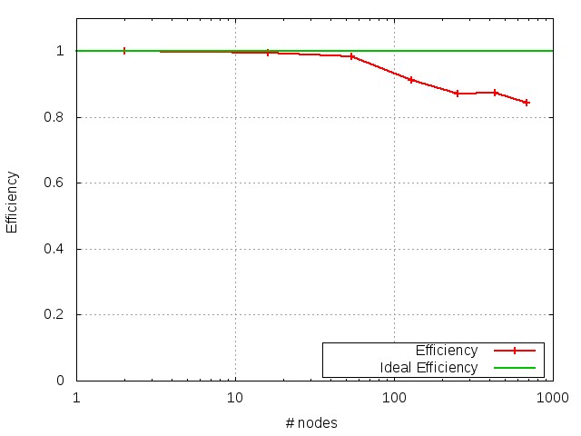
In Fig. 6 weak scaling results are presented using gridpoints per task, 4 task per node, 17 threads per task. A reasonably good performance, a parallel efficiency of is obtained using up to nodes, that means a 1.4 PFlops peak performance.
Three different levels of parallelism have to be deployed for an efficient Exascale simulation:
- •
At core/floating point unit level: (e.g., using vectorization)
- •
At node level: (i.e., shared memory parallelization with threads)
- •
At clustRoofKNL.jpeger level: (i.e., distributed memory parallelization with task)
The user must be able to manage all the three levels but the third one depends not only by the user (Sec. 3.3), since the performance crucially depends on the technology and the topology of the network, as well as on the efficiency of the communication software.
5 Tentative ideas
It is often argued that Exascale computing requires a new computational “ecosystem”, meaning by this that hardware, software and computational algorithms, must all work in orchestrated harmony.
The challenges associated with achieving the above task on exascale machines is
likely to require an optimal balance between evolutionary versus revolutionary changes to the
existing algorithms, as well as to the programming models.
For very informative discussions on these topics, see [30, 31, 32].
Besides scalability, the authors point out a number of additional crucial metrics, such
as resilience to failure rates and silent errors, energy-consumption, runtime
reconfigurability, as well as new programming models and languages
aimed at supporting the above metrics.
In the following, we present some potentially new ideas on the specific
topics of communication/computation overlap and fault-tolerance in prospective
exascale LB applications.
5.1 Time-delayed LB
The idea of time-delayed PDE’s as a means of further hiding communication costs has been recently put forward by Ansumali and collaborators [25]. The main point is to apply the Liouvillean operator at a delayed past time , namely:
| (9) |
A formal Taylor expansion shows that this is tantamount to advancing the
system at time via a retarded Liouvillean .
The delay provides a longer lapse between the posting of data request
(non-blocking send/receive) and the actual reception, thereby leaving more time for
doing additional work, while waiting for the requested data.
In the case of LB, a M-level delayed streaming would look like follows
| (10) |
where are suitable normalized weights.
Incidentally, we note that for a negative-definite , as required by stability,
is a dilatation of for any .
Therefore, besides introducing extra higher-order errors, the delayed scheme
is subject to more stringent stability constraints than the standard one-time level version.
Nevertheless, once these issues are properly in place, delayed versions of LB might
prove very beneficial for Exascale implementations.
5.2 Fault-tolerant LB
Another crucial issue in the Exascale agenda is to equip the computational model with
error-recovery procedures, assisting the standard hardware operation
against fault occurrences and silent errors (so far, hardware took up the full job).
Due to the large number of nodes/core, HW faults are very likely to appear routinely
by a mere statistical argument [31].
As a consequence, not only at system level all libraries & API (e.g., MPI) have
to be robust and fault-tolerant, but also the computational scheme.
To the best of our knowledge, for the case of LB, this key issue is entirely
unexplored at the time of this writing.
5.2.1 Check-Point Restart protocols
The standard strategy to recover from system failures is Check-Point Restart (CPR), i.e. roll the system back to the closest checkpoint and resume execution from there. The CPR strategy is error-free, but very costly, since it requires a periodic dump of the full system configuration, easily in the order of tens of thousands trillions variables for Exascale applications (say, a cube of linear size lattice units).
The frequency at which CPR must take place is strictly related to the expected
failure rate of the system, which is a pretty complex quantity to assess.
However, at a failure rate of about two per hour, as recently predicted on
for exascale platforms[32], an exaflops/s LB simulation with
lattice sites, each taking flops/site/step, would advance
one timestep per second, which means about CPR every steps.
Although this is well separated from the simulation timescale, it places nonetheless
a major strain on the I/O subsystem, as we are talking of the order of 1 Exabyte for each CPR.
A less-conservative but more sustainable procedure, consists of injecting a correction term at the time
when the error is first detected and keep going from there, without any roll-back, a
strategy sometimes referred to as imprecise computing.
The close-eyes hope is that a suitable correction term can be extrapolated from the
past, and that the error still left shows capable of self-healing within a reasonably short transient time.
The first question is: how should such correction term look like?
Here comes a tentative idea.
Let be the time of most recent check-point and the time
of error-detection (ED). One could estimate the reconstructed ED state by
time-extrapolating from to .
Formally
| (11) |
where denotes some suitable Predictor operator, extrapolating from to .
This assumes the availability of a sequence of outputs , where .
Generally, that sequence is available but restricted to a set of hydrodynamic fields, say for short, such
as density and fluid velocity, namely four fields instead of twenty or so, major savings.
Density and velocity are sufficient to reconstruct the equilibrium component but
not the full distribution , because the non-equilibrium component depends
on the gradients (in principle at all orders) of the equilibrium.
One could then partially reconstruct by taking first order gradients of density
and velocity, a procedure which is going particularly touchy near the boundaries.
Here a peculiar feature of LB may prove pretty helpful: the first order gradients do not need to
be computed since they are contained in the momentum flux tensor, defined as
, a local combination of the populations.
If the momentum flux tensor is also stored in the hydrodynamic set , then
the first-order gradient contribution to non-equilibrium is already accounted for, and only higher order
non equilibrium terms, usually called “ghosts” in LB jargon, are left out from the reconstruction.
This is very good news; yet, it does not come for free, since the momentum flux tensor involves
another six fields, for a total of ten, only half of the memory required by the full configuration.
Regardless of which policy is used, the entire procedure hangs on the
(reasonable?) hope that leaving ghosts out of the reconstruction of ,
is not going to compromise the quality of the predicted state .
Although only direct experimentation can tell, one may argue that numerical methods equipped
with inherent stability properties, such as the entropic LB [26],
should stand good chances for fault-tolerant implementations.
For instance, restricting the predicted solution to feature an entropy increase (or
non-decrease) as compared to the current state at time , may help improve
the quality of the reconstruction procedure.
It should also be pointed out that higher-order moments can also be systematically
reconstructed by suitable recursive procedures exploiting the recurrence
relations between Hermite basis functions [27].
5.2.2 Mitigating Silent Data Corruptions
The above procedures may prove pretty useful not only to design better CPR protocols, but also to mitigate the effects of silent errors, or better said, silent data corruptions (SDC’s). SDC’s are expected to become a major source of concern on exascale systems for a series of reasons, primarily the reduction in size and corresponding increase in number of elementary components, which enhances their exposure to, say, cosmic radiation. A number of studies show that although the majority of SDC’s leads to explicit crashes, a smaller fraction corrupts the results without crashing the application, which is of course way more dangerous [32]. To the best of our knowledge, the vulnerability of LB to SDC’s stands completely unexplored at the time of this writing. Here again, entropic formulations and/or recursive reconstruction of kinetic moments may offer new possibilities. For instance, some errors might remain silent. i.e. escape detection, at the level of lowest order moments but not at the ghost level, so that ghosts could be used as SDC’s detectors.
Summarizing, the kinetic LB representation may offer new physics-inspired data-compression and error-detection/correction strategies to deal with fault-tolerance and silent data corruptions: the exploration of these strategies makes a very interesting research topic for the design of a new generation Exascale LB schemes.
6 Prospective Exascale LB applications
In the present paper, we have discussed at length the challenges faced by LB to meet
with Exascale requirements.
Given that, as we hope we have been able to show, this is not going to be
a plain “analytic continuation of current LB’s”, the obvious question before
concluding is: what can we do once Exascale LB is with us?
The applications are indeed many and most exciting.
For instance, Exascale LB codes will enable direct numerical simulations
at Reynolds numbers around , thereby relieving much work from turbulence models.
The full-scale design of automobiles will become possible.
At moderate Reynolds regimes, Exascale hemodynamics will permit to simulate a full heartbeat
at red-blood cell resolution in about half an hour, thus disclosing new
opportunities for precision medicine.
Likewise, Exascale LB-particle codes will allow millisecond simulations of protein dynamics within the
cell, thereby unravelling invaluable information on many-body hydrodynamic effects under crowded conditions,
which are vital to many essential biological functions, hence potentially also for medical therapies
against neurological diseases [28].
Further applications can be envisaged in micro-nanofluidics, such as the simulation of foams
and emulsions at near-molecular resolution, so as to provide a much more detailed
account of near-contact interface interactions, which are essential to understand the complex rheology of such flows.
For instance, the macroscale structure (say mm) of soft-flowing crystals, i.e., ordered collections of liquid droplets
within a liquid solvent (say oil in water), is highly sensitive to the nanoscale interactions which take place
as interfaces come in near-contact, thereby configuring a highly challenging multiscale problem spanning
six spatial decades and nearly twice as many in time [34].
As a very short example, Fig.7 shows different configurations of monodispersed emulsions at the outlet of
the flow-focuser obtained by changing the dispersed/continuous flow rate ratios.
Such multiscale problem is currently handled via a combination of coarse-graining and grid-refinement techniques [29].
Exascale computing would drastically relax the need for both, if not lift it altogether, thereby paving the way to
the computational design of mesoscale materials (mm) at near-molecular resolution (nm) [8].
The prospects look bright and exciting, but a new generation of ideas and
LB codes are needed to turn this mind-boggling potential into a solid reality.



References
- [1] T. Kurth, S. Treichler et al, Exascale Deep Learning for Climate Analytics https://arxiv.org/abs/1810.01993 (2018).
- [2] S. Succi, The Lattice Boltzmann Equation - For Complex States of Flowing Matter, Oxford University Press, (2018).
- [3] A. Montessori, P. Prestininzi et al., Lattice Boltzmann approach for complex nonequilibrium flows, Phys. Rev. E 92 (4), 043308 (2015)
- [4] S Succi, The European Physical Journal B 64 (3-4), 471-479 74 (2008)
- [5] S. Succi, Lattice Boltzmann 2038. EPL, 109 50001 (2015)
- [6] T. Kruger, H. Kusumaatmaja et al., The Lattice Boltzmann Method Principles and Practice, Springer (2017)
- [7] A. Montessori, G. Falcucci, Lattice Boltzmann Modeling of Complex Flows for Engineering Applications Morgan & Claypool Publishers, (2018)
- [8] A. Montessori, M. Lauricella et al., Elucidating the mechanism of step emulsification, Phys. Rev. Fluids 3, 072202(R) (2018)
- [9] S. Chen and D. Martínez, On boundary conditions in lattice Boltzmann methods Physics of Fluids 8, 2527 (1996)
- [10] lM.Wittmann, V.Haag at al., LBM Lattice Boltzmann benchmark kernels as a testbed for performance analysis, Computers & Fluids Volume 172, Pages 582-592 (2018)
- [11] G. S. Aniruddha, K. Siddarth et al., On vectorization of lattice based simulation, Int. J. of Modern Physics C Vol. 24, No. 12, 1340011 (2013)
- [12] K. Mattila, J. Hyväluoma et al., Comparison of implementations of the lattice-Boltzmann method, Computers & Math. with Applications, Vol. 55, 7, Pp 1514-1524 (2008)
- [13] F. Massaioli, G. Amati, Achieving high performance in a LBM code using OpenMP, The 4th European Workshop on OpenMP (http://www.compunity.org/events/pastevents/ewomp2002/EWOMP02-09-1_massaioli_amati_paper.pdf) (2002)
- [14] M. Bernaschi, S. Melchionna et al., MUPHY: A parallel MUlti PHYsics/scale code for high performance bio-fluidic simulations, Comp. Phys. Comm., Vol. 180, 9, pp. 1495-1502, (2009)
- [15] F. Schornbaum, U. Rüde: Massively Parallel Algorithms for the Lattice Boltzmann Method on Nonuniform Grids, SIAM Journal on Scientific Computing, 38(2): 96-126, 2016
- [16] G. E. Moore, Progress in digital integrated electronics, Electron Devices Meeting (1975)
- [17] https://www.top500.org/
- [18] S. Williams, A. Waterman et al., Roofline: an insightful visual performance model for multicore architectures, Communications of the ACM, Vol. 52, 4, pp.65-76, (2009)
- [19] A. Sodani, R. Gramunt et al., Knights Landing: Second-Generation Intel Xeon Phi Product, IEEE Micro, Vol. 36, 2 (2016)
- [20] J. D. McCalpin, Memory Bandwidth and System Balance in HPC systems, http://sites.utexas.edu/jdm4372/2016/11/22/sc16-invited-talk-memory-bandwidth-and-system-balance-in-hpc-systems/.
- [21] VK. Krastev, G. Amati, et al. On the effects of surface corrugation on the hydrodynamic performance of cylindrical rigid structures, Eur. Phys. J. E 41: 95 (2018)
- [22] D. Lagrava, O. Malaspinas et al., Advances in multi-domain lattice Boltzmann grid refinement, J. of Comput. Physics, Volume 231, 14, Pp 4808-4822 (2012)
- [23] http://www.hpc.cineca.it/hardware/marconi
- [24] X. Shan. H. Chen, Lattice Boltzmann model for simulating flows with multiple phases and components, Phys. Rev. E 47, 1815, (1993)
- [25] D. Mudigere, S. D. Sherlekar, et al., Delayed Difference Scheme for Large Scale Scientific Simulations Phys. Rev. Lett. 113, 218701 (2014)
- [26] S. Chikatamarla, S. Ansumali, et al., Entropic Lattice Boltzmann Models for Hydrodynamics in Three Dimensions, Phys. Rev. Lett. 97, 010201 (2006)
- [27] Coreixas C , Wissocq G , et al. Recursive regularization step for high-order lattice Boltzmann methods, Phys. Rev. E, 96,033306 (2017).
- [28] M. Bernaschi, S. Melchionna et al., Mesoscopic simulations at the physics-chemistry-biology interface. Rev. Mod. Phys., 91(2), 025004 (2019).
- [29] A. Montessori et al, Mesoscale modelling of soft flowing crystals, Phil. Trans. A, Accepted, DOI 10.1098/rsta.2018.0149, 2018
- [30] Da Costa, Fahringer, et al., Exascale machines require new programming paradigms and runtimes, Supercomputing frontiers and innovations, 2, 6-27, (2015).
- [31] F. Cappello, A. Geist, W. Gropp et al, Towards Exascale Resilience, Int. J. High Perform. Comput. Appl., 23(4), 374, (2014).
- [32] M. Snir, R.W. Wisniewski, J. A. Abrahm et al, Addressing failures in exascale computing, Int. J. High Perform. Comput. Appl., 28(2) 129, (2014).
- [33] P.L. Guhur, E. Constantinescu, D. Ghosh et al, Detection of Silent Data Corruption in Adaptive Numerical Integration Solvers, IEEE International Conference on Cluster Computing (CLUSTER). IEEE, 592, (2017).
- [34] A. Montessori, M. Lauricella and S. Succi, Mesoscale modelling of soft-flowing crystals, Phil. Trans. Roy. Soc. A, 377(2142), 20180149, (2019).