Functions and eigenvectors of partially known matrices with applications to network analysis
Abstract
Matrix functions play an important role in applied mathematics. In network analysis, in particular, the exponential of the adjacency matrix associated with a network provides valuable information about connectivity, as well as about the relative importance or centrality of nodes. Another popular approach to rank the nodes of a network is to compute the left Perron vector of the adjacency matrix for the network. The present article addresses the problem of evaluating matrix functions, as well as computing an approximation to the left Perron vector, when only some of the columns and/or some of the rows of the adjacency matrix are known. Applications to network analysis are considered, when only some sampled columns and/or rows of the adjacency matrix that defines the network are available. A sampling scheme that takes the connectivity of the network into account is described. Computed examples illustrate the performance of the methods discussed.
keywords
Matrix function, Arnoldi process, low-rank approximation, cross approximation, column subset selection, centrality measure1 Introduction
Many problems in applied mathematics can be formulated and solved with the aid of matrix functions. This includes the solution of linear discrete ill-posed problems [7], the solution of time-dependent partial differential equations [12], and the determination of the most important node(s) of a network that is represented by a graph and its adjacency matrix [13, 15]. Usually, all entries of the adjacency matrix are assumed to be known. This paper is concerned with the situation when only some columns, and/or rows, of the matrix are available. This situation arises, for instance, when one samples columns, and possibly rows, of a large matrix. We will consider applications in network analysis, where column and/or row sampling arises naturally in the process of collecting network data by accessing one node at a time and finding all the other nodes it is connected to. This is particularly important when it is too expensive or impractical to collect a full census of all the connections.
A network is represented by a graph , which consists of a set of vertices or nodes, and a set of edges, the latter being the links between the vertices. Edges may be directed, in which case they emerge from a node and end at a node, or undirected. Undirected edges are “two-way streets” between nodes. For notational convenience and ease of discussion, we consider simple (directed or undirected) unweighted graphs without self-loops. Then the adjacency matrix associated with the graph has the entry if there is a directed edge emerging from vertex and ending at vertex ; if there is an undirected edge between the vertices and , then . Other matrix entries vanish. In particular, the diagonal entries of vanish. Typically, , which makes the matrix sparse. A graph is said to be undirected if all its edges are undirected, otherwise the graph is directed. The adjacency matrix for an undirected graph is symmetric; for a directed graph it is nonsymmetric. Examples of networks include:
- •
Flight networks, with airports represented by vertices and flights by directed edges.
- •
Social networking services, such as Facebook and Twitter, with members or accounts represented by vertices and interactions between any two accounts by edges.
Numerous applications of networks are described in [9, 14, 26].
We are concerned with the situation when only some of the nodes and edges of a graph are known. Each node and its connections to other nodes determine one row and column of the matrix . Specifically, all edges that point to node determine column of , and all edges that emerge from this node define the row of . We are interested in studying properties of networks associated with partially known adjacency matrices.
An important task in network analysis is to determine which vertices of an associated graph are the most important ones by measuring how well-connected they are to other vertices of the graph. This kind of importance measure often is referred to as a centrality measure. The choice of a suitable centrality measure depends on what the graph is modeling. All commonly used centrality measures ignore intrinsic properties of the vertices, and provide information about their importance within the graph just by using connectivity information.
A simple approach to measure the centrality of a vertex in a directed graph is to count the number of edges that point to it. This number is known as the indegree of . Similarly, the outdegree of is the number of edges that emerge from this vertex. For undirected graphs, the degree of a vertex is the number of edges that “touch” it. However, this approach to measure the centrality of a vertex often is unsatisfactory, because it ignores the importance of the vertices that is connected to. Here we consider the computation of certain centrality indices quantifying the “importance” of a vertex on the basis of the importance of its neighbors, according to different criteria of propagation of the vertex importance. Such centrality indices are based on matrix functions of the adjacency matrix of the graph, and are usually called spectral centrality indices. In particular, we focus on the Katz index and the subgraph centrality index. Moreover, we also consider eigenvector centrality, that is, the Perron eigenvector of the adjacency matrix.
To discuss measures determined by matrix functions, we need the notion of a walk in a graph. A walk of length is a sequence of vertices and a sequence of edges , such that points from to for . The vertices and edges of a walk do not have to be distinct. It is a well known fact that , i.e., the entry of , yields the number of walks of length starting at node and ending at node . Thus, a matrix function evaluated at the adjacency matrix , defined by a power series with nonnegative coefficients, can be interpreted as containing weighted sums of walk counts, with weights depending on the length of the walk. Unless is nilpotent (i.e., the graph is directed and contains no cycles), convergence of the power series requires that the coefficients converge to zero; this corresponds well with the intuitively natural requirement that long walks be given less weight than short walks (which is the case in (1) and (2) below).
Commonly used matrix functions for measuring the centrality of the vertices of a graph are the exponential function and the resolvent , where and are positive user-chosen scaling parameters; see, e.g., [13]. These functions can be defined by their power series expansions
| (1) | |||||
| (2) |
For the resolvent, the parameter has to be chosen small enough so that the power series converges, which is the case when is strictly smaller than , where denotes the spectral radius of .
Matrix functions , such as (1) and (2), define several commonly used centrality measures: If , then is called the total subgraph communicability of node , while the diagonal matrix entry is the subgraph centrality of node ; see, e.g., [2, 13]. Moreover, if , then gives the Katz index of node ; see, e.g., [26, Chap. 7].
It may be beneficial to complement the centrality measures above by the measures and , , when the graph that defines is directed. Here and below the superscript T denotes transposition; see, e.g., [2, 11, 13, 14] for discussions on centrality measures defined by functions of the adjacency matrix.
We are interested in computing useful approximations of the largest diagonal entries of , or the largest entry of or , when only of the columns and/or rows of are known. The need to compute such approximations arises when the entire graph is not completely known, but only a small subset of the columns or rows of the adjacency matrix of are available. This happens, e.g., when not all nodes and edges of a graph are known, a situation that is common for large, complex, real-life networks. The situation we will consider is when the columns and rows of the adjacency matrix are not explicitly known, but can be sampled. It is then of considerable interest to investigate how the sampling should be carried out, as simple random sampling of columns and possibly rows of a large adjacency matrix does not give the best results. We will describe a sampling method in Section 2. A further reason for our interest in computing approximations of functions of a large matrix , that only use a few of the columns and/or rows of the matrix, is that the evaluation of these approximations typically is much cheaper than the evaluation of functions of .
Another approach to measure centrality is to compute a left or right eigenvector associated with the eigenvalue of largest magnitude of . In many situations the entries of these eigenvectors live in a one-dimensional invariant subspace, have only nonvanishing entries, and can be scaled so that all entries are positive. The so-scaled eigenvectors are commonly referred to as the left and right Perron vectors for the adjacency matrix . The left and right Perron vectors are unique up to scaling provided that the adjacency matrix is irreducible or, equivalently, if the associated graph is strongly connected. The centrality of a node is given by the relative size of its associated entry of the (left or right) Perron vector for the adjacency matrix. If the entry of the, say left, Perron vector is the largest, then is the most important vertex of the graph. This approach to determine node importance is known as eigenvector centrality or Bonacich centrality; see, e.g., [3, 14, 26] for discussions of this method. We will consider the application of this method to partially known adjacency matrices.
This paper is organized as follows. Section 2 discusses our sampling method for determining (partial) knowledge of the graph and its associated adjacency matrix. The evaluation of matrix functions of adjacency matrices that are only partially known is considered in Section 3, and Section 4 describes how an approximation of the left Perron vector of can be computed quite inexpensively by using low-rank approximations determined by sampling. A few computed examples are presented in Section 5, and concluding remarks can be found in Section 6.
2 Sampling adjacency matrices
Let be the singular values of a large matrix and let, for some , and be left and right singular (unit) vectors associated with the largest singular values. Then the truncated singular value decomposition (TSVD)
| (3) |
furnishes a best approximation of of rank at most with respect to the spectral and Frobenius matrix norms; see, e.g., [33]. However, the computation of the approximation (3) may be expensive when is large and is of moderate size. This limits the applicability of the TSVD-approximant (3). Moreover, the evaluation of this approximant requires that all entries of be explicitly known.
As mentioned above, we are concerned with the situation when is an adjacency matrix for a simple (directed or undirected) unweighted graph without self-loops and that, while the whole matrix is not known, we can sample a (relatively small) number of rows and columns. Then, approximations different from (3) have to be used. This section discusses methods to sample columns and/or rows of . The low-rank approximations of determined in this manner are used in Sections 3 and 4 to compute approximations of spectral node centralities.
In the first step, a random non-vanishing column of is chosen. Let its index be , and denote the chosen column by . If the columns have been chosen, corresponding to the indices , at the next step we pick an index according to a probability distribution on proportional to . Thus, at the step, the probability of choosing column as the next sampled column is proportional to the number of edges in the network from node to nodes . At each step, if a column has already been picked, or the new column consists entirely of zeros, this choice is discarded and the procedure is repeated until a new, nonzero column is obtained. We denote by the set of indices of the chosen columns; using MATLAB notation, the matrix is made up of the chosen columns of . Another way of describing this sampling method is that we pick the first vertex at random, and then pick subsequent vertices randomly using a probability distribution proportional to .
We remark that this scheme for selecting columns can just as easily be used in the case when the edges have positive weights (that is, the nonzero entries of may be positive numbers other than 1). Also, if a row-sampling scheme is needed, rows of the adjacency matrix can be selected similarly by applying the above scheme to the columns of the matrix ; in this case we denote by the set of row indices. The matrix contains the selected rows of . By alternating column and row sampling, sets of columns and rows can be determined simultaneously.
The adaptive cross approximation method (ACA) applied to a matrix also samples rows and columns to obtain an approximation of the whole matrix. In ACA, one uses the fact that the rows and columns of and have common entries. These entries form the matrix . When the latter matrix is nonsingular, the cross approximation of is given by
| (4) |
Let be the singular value of . Then the matrix (3) satisfies , where denotes the spectral norm. Goreinov et al. [18] show that there is a matrix of rank , determined by cross approximation of , such that
| (5) |
Thus, cross approximation can determine a near-best approximation of of rank without computing the first singular values and vectors of .
However, the selection of columns and rows of so that (5) holds is computationally difficult. In their analysis, Goreinov et al. [19] select sets and that give the submatrix maximal “volume” (modulus of the determinant). It is difficult to compute these index sets in a fast manner. Therefore, other methods to select the sets and have been proposed; see, e.g., [16, 24]. They are related to incomplete Gaussian elimination with complete pivoting. These methods work well when the matrix is not very sparse. The adjacency matrices of concern in the present paper typically are quite sparse, and we found the sampling methods described in [16, 24] often to give singular matrices . This makes the use of adaptive cross approximation difficult. We therefore will not use the expression (4) in subsequent sections.
3 Functions of low-rank matrix approximations
This section discusses the approximation of functions of a large matrix that is only partially known. Specifically, we assume that only columns of are available, and we would like to determine an approximation of . We will tacitly assume that the function and matrix are such that is well defined; see, e.g., [17, 20] for several definitions of matrix functions. For the purpose of this paper, the definition of a matrix function by its power series expansion suffices; cf. (1) and (2). We first will assume that the matrix is nonsymmetric. At the end of this section, we will address the situation when is symmetric.
Let be a permutation matrix such that the known columns of the matrix have indices . Thus, the first columns of are . Let for . We first approximate by
| (6) |
Thus,
and then approximate by
| (7) |
Hence, it suffices to consider the evaluation of at an matrix, whose last columns vanish. We will tacitly assume that is well defined.
The computations simplify when . We therefore will consider the functions
| (8) |
The subtraction of in the above expressions generally is of no significance for the analysis of networks, because one typically is interested in the relative sizes of the diagonal entries of , or of the entries of the vectors or .
The power series representations of the functions in (8),
show that only the first columns of the matrix contain nonvanishing entries.
Let be a random unit vector (not belonging to ). Application of steps of the Arnoldi process to with initial vector , generically, yields the Arnoldi decomposition
| (9) |
where is an upper Hessenberg matrix and the matrix has orthonormal columns. The computation of the Arnoldi decomposition (9) requires the evaluation of matrix-vector products with , which is quite inexpensive since has at most nonvanishing columns. We assume that the decomposition (9) exists. This is the generic situation. Breakdown of the Arnoldi process, generically, occurs at step ; see Saad [30, Chapter 6] for a thorough discussion of the Arnoldi decomposition and its computation.
Introduce the spectral factorization
| (10) |
which we tacitly assume to exist. This is the generic situation. Thus, the matrix is diagonal; its diagonal entries are the eigenvalues of . We may assume that the eigenvalues are ordered by nonincreasing modulus. Then the last diagonal entry of vanishes. It follows that the last column of the matrix is an eigenvector that is associated with a vanishing eigenvalue. There may be other vanishing diagonal entries of as well, but this will not be exploited. The situation when the factorization (10) does not exist can be handled as described by Pozza et al. [28].
We have
The columns of are eigenvectors of . The last column of is an eigenvector that is associated with a vanishing eigenvalue.
Let , , where denotes the column of an identity matrix of appropriate order. Then
is an eigenvector matrix of , and
where is the leading principal submatrix of . Hence,
| (11) | |||||
where we have used the fact that .
To evaluate the expression (11), it remains to determine the first rows of . This can be done with the aid of the Sherman–Morrison–Woodbury formulas [17, p. 65]. Define the matrix and let denote the leading principal submatrix of the identity matrix . Then the first rows of are given by , and we can evaluate
| (12) |
where denotes a matrix with only zero entries.
Our approximation of is given by . For a large matrix , the computationally most expensive part of evaluating this approximation, when the matrix is available, is the computation of the Arnoldi decomposition (9), which requires arithmetic floating point operations.
We remark that for functions such that
| (13) |
which includes the functions (1) and (2), we may instead sample rows of , which are columns of , to determine an approximation of using the same approach as described above. We remark that equation (13) holds for all matrix functions that stem from a scalar function for .
We turn to the situation when the matrix is symmetric, and assume that of its columns are known. Let the permutation matrix be the same as above. Then the first rows and columns of the symmetric matrix are available. Letting be a random unit vector and applying steps of the symmetric Lanczos process to with initial vector gives, generically, the Lanczos decomposition
| (14) |
where is a symmetric tridiagonal matrix and has orthonormal columns. The computation of the decomposition (14) requires the evaluation of matrix-vector products with . We assume is small enough so that the decomposition (14) exists. Breakdown depends on the choice of . Typically this assumption is satisfied; otherwise the computations can be modified. Breakdown of the symmetric Lanczos process, generically, occurs at step . We now can derive a representation of of the form (11), making use of the spectral factorization of . The derivation in the present situation is analogous to the derivation of in (11), with the difference that the eigenvector matrix can be chosen to be orthogonal.
4 The computation of an approximate left Perron vector
Let be the adjacency matrix of a strongly connected graph. Then has a unique left Perron vector of unit length with all entries positive. As mentioned above, the importance of vertex is proportional to . When the matrix is nonsymmetric, the left Perron vector measures the centrality of the nodes as receivers; the right Perron vector yield the centrality of the nodes as transmitters.
Assume for the moment that the (unmodified) adjacency matrix is nonsymmetric. We would like to determine an approximation of the left Perron vector by using a submatrix determined by sampling columns and rows as described in Section 2. Let the set contain the indices of the sampled columns of . Thus, the matrix contains the sampled columns. Similarly, applying the same column sampling method to gives a set of indices; the matrix contains the sampled rows. We will compute an approximation of the left Perron vector of by applying the power method to the matrix , which approximates (without explicitly forming ). We instead also could have applied the power method to . Since the matrix is not explicitly stored, the latter choice offers no advantage.
Possible nonunicity of the Perron vector and non-convergence of the power method can be remedied by adding a matrix to , where all entries of are equal to a small parameter . The computations with the power method are carried out without explicitly storing the matrix and forming . The iterations with the power method applied to are much cheaper than the iterations with the power method applied to , when . Moreover, our method does not require the whole matrix to be explicitly known. In the computed examples reported in Section 5, we achieved fairly accurate rankings of the most important nodes without using the matrix defined above. Moreover, we found that only fairly few rows and columns of were needed to quite accurately determine the most important nodes in several “real” examples.
When the adjacency matrix is symmetric, we propose to compute the Perron vector of the matrix , which can be constructed by sampling the columns of , only, to construct , since . Notice that for symmetric matrices the right and left Perron vectors are the same.
5 Computed examples
This section illustrates the performance of the methods discussed when applied to the ranking of nodes in several “real” large networks. All computations were carried out in MATLAB with standard IEEE754 machine arithmetic on a Microsoft Windows 10 computer with CPU Intel(R) Core(TM) i7-8550U @ 1.80GHz, 4 Cores, 8 Logical Processors and 16GB of RAM.


| Mean | Max | Min | |
|---|---|---|---|
| 500 | 22.28 | 24.05 | 17.23 |
| 1000 | 85.28 | 93.33 | 74.20 |
| 1500 | 184.46 | 189.55 | 177.92 |
| 2000 | 336.34 | 477.35 | 323.31 |
| 2500 | 549.49 | 596.81 | 524.38 |
| 3000 | 753.24 | 810.85 | 721.24 |
5.1 soc-Epinions1
The network of this example is a “web of trust” among members of the website Epinions.com. This network describes who-trusts-whom. Each user may decide to trust the reviews of other users or not. The users are represented by nodes. An edge from node to node indicates that user trusts user . The network is directed with 75,888 members (nodes) and 508,837 trust connections (edges) [29, 31]. We will illustrate that one can determine a fairly accurate ranking of the nodes by only using a fairly small number of columns of the nonsymmetric adjacency matrix with . The node centrality is determined by evaluating approximations of the diagonal entries of the matrix function .
We sample columns of the adjacency matrix using the method described in Section 2. The first column, , is a randomly chosen nonvanishing column of ; the remaining columns are chosen as described in Section 2. Once the columns of have been chosen, we evaluate an approximation of as described in Section 3. The rankings obtained are displayed in Figure 1; see below for a detailed description of this figure. When instead all columns of are chosen randomly, then we obtain the rankings shown in Figure 2. Computing times are reported in Table 1.
The exact ranking of the nodes of the network is difficult to determine due to the large size of the adjacency matrix. It is problematic to evaluate both because of the large amount of computational arithmetic required, and because of the large storage demand. While the matrix is sparse, and therefore can be stored efficiently using a sparse storage format, the matrix is dense. In fact, the MATLAB function expm cannot be applied to evaluate on the computer used for the numerical experiments. Instead, we apply the Arnoldi process to approximate . Specifically, steps of the Arnoldi process applied to with a random unit initial vector generically gives the Arnoldi decomposition
| (15) |
where the matrix has orthonormal columns, is an upper Hessenberg matrix, and the vector is orthogonal to the columns of . We then approximate by ; see, e.g., [1, 12] for discussions on the approximation of matrix function using the Arnoldi process. These computations were carried out for , , , and , and rankings for these -values were determined. We found the rankings to converge as increases. The ranking obtained for therefore is considered the “exact” ranking. It is shown in the second column of Figure 1. Subsequent columns of this figure display rankings determined by the diagonal entries of for , , , , , and , when the columns of are sampled by the method of Section 2. Each column shows the top 20 ranked nodes. To make it easier for a reader to see the rankings, we use colors, and levels for each color. As we pick columns of , of the top ranked nodes are identified, but only the most important node (35) has the correct ranking. When , the computed ranking improves somewhat. We are able to identify out of top nodes. As we sample more columns of , we obtain improved rankings. For , we are able to identify of the most important nodes, and the rankings get closer to the exact ranking. The figure illustrates that useful information about node centrality can be determined by sampling many fewer than columns of . Computing times are reported in Table 1.
Figure 2 differs from Figure 1 in that the columns of the matrix are randomly sampled. Comparing these figures shows the sampling method of Section 2 to yield rankings that are closer to the “exact ranking” of the second column for the same number of sampled columns.

| Mean | Max | Min | |
|---|---|---|---|
| 500 | 0.89 | 1.02 | 0.76 |
| 1000 | 2.38 | 3.54 | 2.06 |
| 1500 | 4.61 | 7.66 | 3.55 |
| 2000 | 7.55 | 12.43 | 5.78 |
| 2500 | 10.87 | 19.45 | 8.45 |
| 3000 | 15.53 | 37.50 | 11.03 |
5.2 ca-CondMat
This example illustrates the application of the technique of Section 3 to a symmetric partially known matrix. We consider a collaboration network from e-print arXiv. The 23,133 nodes of the associated graph represent authors. If author co-authored a paper with author , then the graph has an undirected edge connecting the nodes and . The adjacency matrix is symmetric with 186,936 non-zero entries [23, 31]. Of the entries, 58 are on the diagonal. Since we are interested in graphs without self-loops, we set the latter entries to zero. We use the node centrality measure furnished by the diagonal of .
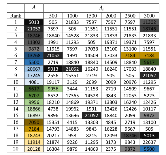
Figure 3 shows results when using the sampling method described in Section 2 to choose columns of the adjacency matrix . Due to the symmetry of , we also know rows of . The figure compares the ranking of the nodes using the diagonal of the matrix (which is the exact ranking) with the rankings determined by the diagonal entries of for . The figure shows the top ranked nodes determined by each matrix. For , a couple of the most important nodes can be identified among the first nodes, but their rankings are incorrect. The most important node (5013) is in the position, and the second most important node (21052) is in the position. Increasing to 1000 yields more accurate rankings. The most important nodes, i.e., (5013), (21052), and (18746), are ranked correctly. Increasing further yields rankings that are closer to the “exact” ranking of the second column. For instance, identifies of the most important nodes, and of them have the correct rank. The figure suggests that we may gain valuable insight into the ranking of the nodes by using fairly few columns (and rows) of the adjacency matrix, only. Computing times are shown in Table 2.
Figure 4 differs from Figure 3 in that the columns of the matrix are randomly sampled. Comparing these figures shows that the sampling method of Section 2 gives rankings that are closer to the “exact ranking” of the second column for the same number of sampled columns.

| Mean | Max | Min | |
|---|---|---|---|
| 500 | 0.21 | 0.37 | 0.11 |
| 1000 | 0.32 | 0.58 | 0.10 |
| 1500 | 0.38 | 0.66 | 0.10 |
| 2000 | 0.42 | 0.72 | 0.10 |
| 2500 | 0.42 | 0.84 | 0.11 |
| 3000 | 0.43 | 0.95 | 0.10 |
5.3 Enron
This example illustrates the application of the method described in Section 4 to a nonsymmetric adjacency matrix. The network in this example is an e-mail exchange network, which represents e-mails (edges) sent between Enron employees (nodes). The associated graph is unweighted and directed with 69,244 nodes and 276,143 edges, including 1,535 self-loops. We removed the self-loops before running the experiment. This network has been studied in [10] and can be found at [32].
We choose columns of the matrix as described in Section 2 and put the indices of these columns in the index set . Similarly, we select columns of the matrix . The indices of these rows make up the set . This determines the matrix of rank at most . We calculate an approximation of a left Perron vector of by computing a left Perron vector of . The size of the entries of the Perron vectors determines the ranking.
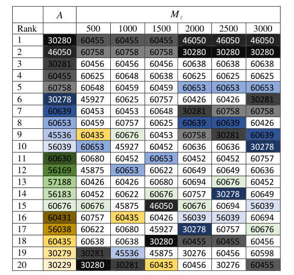
The second column of Figure 5 shows the “exact ranking” determined by a left Perron vector of . The remaining columns show the rankings defined by Perron vectors of for with the sampling of the columns of carried out as described in Section 2. The ranking determined by Perron vectors of gets closer to the exact ranking in the second column as increases. When , we are able to identify out of the most important nodes, but not in the correct order. The three most important nodes have the correct ranking for . When , we almost can identify all the 20 important nodes, because node (60606) is actually ranked . Computing times are shown in Table 3.
Figure 6 differs from Figure 5 in that the columns of the matrix are randomly sampled. These figures show that the sampling method of Section 2 gives rankings that are closer to the “exact ranking” of the second column for the same number of sampled columns.


| Mean | Max | Min | |
|---|---|---|---|
| 500 | 0.08 | 0.13 | 0.03 |
| 1000 | 0.13 | 0.17 | 0.02 |
| 1500 | 0.16 | 0.24 | 0.03 |
| 2000 | 0.19 | 0.26 | 0.03 |
| 2500 | 0.21 | 0.25 | 0.03 |
| 3000 | 0.23 | 0.28 | 0.03 |
5.4 Cond-mat-2005
The network in this example models a collaboration network of scientists posting preprints in the condensed matter archive at www.arxiv.org. It is discussed in [27] and can be found at [25]. We use an unweighted version of the network. The associated graph is undirected and has 40,421 nodes and 351,382 edges. We use the Perron vector as a centrality measure, and compare the node ranking using the Perron vector of with the ranking determined by the Perron vector for the matrices for several -values. The matrix is determined as described in Section 2, and is just .
Figure 7 shows the (exact) ranking obtained with the Perron vector for (2nd column) and the rankings determined by the Perron vector for , for , when the columns of are sampled as described in Section 2. We compare the ranking of the top ranked nodes in these rankings. When , the two most important nodes are ranked correctly by using the Perron vector for . Moreover, out of top ranked nodes are identified, but their ranking is not correct. For , the nine most important nodes are ranked correctly. Computing times are displayed in Table 4.
Figure 8 differs from Figure 7 in that the columns of the matrix are randomly sampled. Clearly, the sampling method of Section 2 gives rankings that are closer to the “exact ranking” for the same number of sampled columns.
The above examples illustrate that valuable information about the ranking of nodes can be gained by sampling columns and rows of the adjacency matrix. The last two examples determine the left Perron vector. The most popular methods for computing this vector for a large adjacency matrix are the power method and enhanced variants of the power method that do not require much computer storage. These methods, of course, also can be applied to determine the left Perron vector of the matrices . It is outside the scope of the present paper to compare approaches to efficiently compute the left Perron vector. Extrapolation and other techniques for accelerating the power method are described in [4, 5, 6, 8, 21, 22, 34].
In our experience the sampling method described performs well on many “real” networks. However, one can construct networks for which sampling might not perform well. For instance, let be an undirected graph made up of two large clusters with many edges between vertices in the same cluster, but only one edge between the clusters. The latter edge may be difficult to detect by sampling and the sampling method. The method therefore might only give results for edges in one of the clusters. We are presently investigating how the performance of the sampling method can be quantified. We would like to mention that the sampling method can be used to study various quantities of interest in network analysis, such as the total communicability [2].
6 Conclusion
In this work we have described novel methods for analyzing large networks in situations when not all of the adjacency matrix is available. This was done by evaluating matrix functions or computing approximations of the Perron vector of partially known matrices. In the computed examples, we considered the situation when only fairly small subsets of columns, or of rows, or both, are known.
There are two distinct advantages to the approaches developed here:
- 1.
They are computationally much cheaper than the evaluation of matrix functions or the computation of the Perron vector of the entire matrix when the adjacency matrix is large.
- 2.
The methods described correspond to a compelling sampling strategy when obtaining the full adjacency information of a network is prohibitively costly. In many realistic scenarios, the easiest way to collect information about a network is to access nodes (e.g., individuals) and interrogating them about the other nodes they are connected to. This version of sequential sampling is described in Section 2.
Finally, in order to illustrate the feasibility of our techniques, we have shown how to approximate well-known node centrality measures for large networks, obtaining quite good approximate node rankings, by using only a few columns and rows of the underlying adjacency matrix.
Acknowledgement
The authors would like to thank Giuseppe Rodriguez and the anonymous referees for comments and suggestions.
References
- [1] B. Beckermann and L. Reichel, Error estimation and evaluation of matrix functions via the Faber transform, SIAM J. Numer. Anal., 47 (2009), pp. 3849–3883.
- [2] M. Benzi and C. Klymko, Total communicability as a centrality measure, J. Complex Networks, 1 (2013), pp. 124–149.
- [3] P. F. Bonacich, Power and centrality: A family of measures, Am. J. Sociol., 92 (1987), pp. 1170–1182.
- [4] C. Brezinski and M. Redivo–Zaglia, Rational extrapolation for the PageRank vector, Math. Comp., 77 (2008), pp. 1585–1598.
- [5] C. Brezinski and M. Redivo–Zaglia, The simplified topological -algorithms for accelerating sequences in a vector space, SIAM J. Sci. Comput., 36 (2014), pp. A2227–A2247.
- [6] C. Brezinski and M. Redivo–Zaglia, The genesis and early developments of Aitken’s process, Shanks’ transformation, the -algorithm, and related fixed point methods, Numer. Algorithms, 80 (2019), pp. 11–133.
- [7] D. Calvetti and L. Reichel, Lanczos-based exponential filtering for discrete ill-posed problems, Numer. Algorithms, 29 (2002), pp. 45–65.
- [8] S. Cipolla, M. Redivo-Zaglia, and F. Tudisco, Shifted and extrapolated power methods for tensor -eigenpairs, Electron. Trans. Numer. Anal., 53 (2020), pp. 1–27.
- [9] J. J. Crofts, E. Estrada, D. J. Higham, and A. Taylor, Mapping directed networks, Electron. Trans. Numer. Anal., 37 (2010), pp. 337–350.
- [10] A. Cruciani, D. Pasquini, G. Amati, and P. Vocca, About Graph Index Compression Techniques, Proceedings of the 10th Italian Information Retrieval Workshop (IIR-2019), Padova, Italy, September 16-18, 2019, CEUR-WS.org/Vol-2441/paper23.pdf.
- [11] O. De la Cruz Cabrera, M. Matar, and L. Reichel, Analysis of directed networks via the matrix exponential, J. Comput. Appl. Math., 355 (2019), pp. 182–192.
- [12] V. Druskin, L. Knizhnerman, and M. Zaslavsky, Solution of large scale evolutionary problems using rational Krylov subspaces with optimized shifts, SIAM J. Sci. Comput., 31 (2009), pp. 3760–3780.
- [13] E. Estrada and D. J. Higham, Network properties revealed through matrix functions, SIAM Rev., 52 (2010), pp. 696–714.
- [14] E. Estrada, The Structure of Complex Networks, Oxford University Press, Oxford, 2012.
- [15] C. Fenu, D. Martin, L. Reichel, and G. Rodriguez, Block Gauss and anti-Gauss quadrature with application to networks, SIAM J. Matrix Anal. Appl., 34 (2013), pp. 1655–1684.
- [16] K. Frederix and M. Van Barel, Solving a large dense linear system by adaptive cross approximation, J. Comput. Appl. Math., 234 (2010), pp. 3181–3195.
- [17] G. H. Golub and C. F. Van Loan, Matrix Computations, th ed., Johns Hopkins University Press, Baltimore, 2013.
- [18] S. A. Goreinov, E. E. Tyrtyshnikov, and N. L. Zamarashkin, A theory of pseudo-skeleton approximation, Linear Algebra Appl., 261 (1997), pp. 1–21.
- [19] S. A. Goreinov, E. E. Tyrtyshnikov, and N. L. Zamarashkin, Pseudo-skeleton approximations by matrices of maximal volume, Math. Notes, 62 (1997), pp. 515–519.
- [20] N. J. Higham, Functions of Matrices: Theory and Computation, SIAM, Philadelphia, 2008.
- [21] K. Jbilou and H. Sadok, LU-implementation of the modified minimal polynomial extrapolation method, IMA J. Numer. Anal., 19 (1999), pp. 549–561.
- [22] K. Jbilou and H. Sadok, Vector extrapolation methods. Applications and numerical comparison, J. Comput. Appl. Math., 122 (2000), pp. 149–165.
- [23] J. Leskovec, J. Kleinberg, and C. Faloutsos, Graph evaluation: Densification and shrinking diameters, ACM Trans. Knowledge Discovery from Data, 1(1) (2007), Art. 2, pp. 1–41.
- [24] T. Mach, L. Reichel, M. Van Barel, and R. Vandebril, Adaptive cross approximation for ill-posed problems, J. Comput. Appl. Math., 303 (2016), pp. 206–217.
- [25] M. E. J. Newman, Network Data, http://www-personal.umich.edu/ mejn/netdata/.
- [26] M. E. J. Newman, Networks: An Introduction, Oxford University Press, Oxford, 2010.
- [27] M. E. J. Newman, The structure of scientific collaboration networks, Proc. Natl. Acad. Sci. USA, 98 (2001), pp. 404–409.
- [28] S. Pozza, M. S. Pranić, and A. Strakoš, The Lanczos algorithm and complex Gauss quadrature, Electron. Trans. Numer. Anal., 48 (2018), pp. 362–372.
- [29] M. Richardson, R. Agrawal, and P. Domingos, Trust management for the semantic web, in The Semantic Web - ISWC 2003, eds. D. Fensel, K. Sycara, and J. Mylopoulos, Lecture Notes in Computer Science, vol. 2870, Springer, Berlin, pp. 351–368.
- [30] Y. Saad, Iterative Methods for Sparse Linear Systems, 2nd ed., SIAM, Philadelphia, 2003.
- [31] Stanford Large Network Dataset Collection, http://snap.stanford.edu/data/index.html
- [32] SuiteSparse Matrix Collection, https://sparse.tamu.edu.
- [33] L. N. Trefethen and D. Bau III, Numerical Linear Algebra, SIAM, Philadelphia, 1997.
- [34] G. Wu, Y. Zhang, and Y. Wei, Accelerating the Arnoldi-type algorithm for the PageRank problem and the ProteinRank problem, J. Sci. Comput., 57 (2013), pp. 74–104.