跳到论文正文
W Papers独立论文阅读器 arXiv:2005.05774 论文正文 计算阅读时间 · 0%
引用这篇论文根据当前论文元数据生成,正式投稿前建议核对。


License: arXiv.org perpetual non-exclusive license
arXiv:2005.05774v1 [math.NA] 12 May 2020

Finite Element Methods For Interface Problems On Local Anisotropic Fitting Mixed MeshesThanks: In this research, Jun Hu was supported by NSFC projects 11625101 and 11421101; Hua Wang was supported by China Postdoctoral Science Foundation Grand 2019M660277 and Jiangsu Key Lab for NSLSCS Grant 201906

Jun Hu Jun HuSchool of Mathematical Sciences, Peking University, Beijing, China Email address: hujun@math.pku.edu.cn and Hua Wang Hua Wang ✉School of Mathematical Sciences, Peking University, Beijing, China Email address: wanghua.math@foxmail.com
Abstract.

A simple and efficient interface-fitted mesh generation algorithm is developed in this paper. This algorithm can produce a local anisotropic fitting mixed mesh which consists of both triangles and quadrilaterals near the interface. A new finite element method is proposed for second order elliptic interface problems based on the resulting mesh. Optimal approximation capabilities on anisotropic elements are proved in both the H1H^{1} and L2L^{2} norms. The discrete system is usually ill-conditioned due to anisotropic and small elements near the interface. Thereupon, a multigrid method is presented to handle this issue. The convergence rate of the multigrid method is shown to be optimal with respect to both the coefficient jump ratio and mesh size. Numerical experiments are presented to demonstrate the theoretical results.

Key words and phrases:
interface-fitted mesh, anisotropic element, multigrid method

1. Introduction

Let Ω\Omega be a convex polygon in ℝ2\mathbb{R}^{2} which is separated by a C2C^{2}-continuous interface Γ\Gamma into two sub-domains Ω1\Omega_{1} and Ω2\Omega_{2}, see Figure 1.1 for an illustration. Consider the following interface problem

(1.1) −div(β∇u)=finΩ1∪Ω2,[[u]]=qonΓ,[[β​∂u∂𝒏Γ]]=gonΓ,u=0on∂Ω,\displaystyle\begin{aligned} -\mathrm{div}(\beta\nabla u)&=f\penalty\ &\mathrm{in}\penalty\ &\Omega_{1}\cup\Omega_{2},\\ [\![u]\!]&=q\penalty\ &\mathrm{on}\penalty\ &\Gamma,\\ [\![\beta\frac{\partial u}{\partial\bm{n}_{\Gamma}}]\!]&=g\penalty\ &\mathrm{on}\penalty\ &\Gamma,\\ u&=0\penalty\ &\mathrm{on}\penalty\ &\partial\Omega,\end{aligned}

where [[v]]:=(v|Ω1)|Γ−(v|Ω2)|Γ[\![v]\!]:=(v|_{\Omega_{1}})|_{\Gamma}-(v|_{\Omega_{2}})|_{\Gamma} for any vv belonging to H1​(Ω1∪Ω2)H^{1}(\Omega_{1}\cup\Omega_{2}), and 𝒏Γ\bm{n}_{\Gamma} is the unit normal vector of Γ\Gamma which points from Ω1\Omega_{1} to Ω2\Omega_{2}, see Figure 1.1. The coefficient function β\beta is discontinuous across the interface Γ\Gamma, i.e.,

(1.2) β={β1,in​Ω1,β2,in​Ω2,\displaystyle\beta=\left\{\begin{aligned} &\beta_{1},\penalty\ \penalty\ \text{in}\penalty\ \Omega_{1},\\ &\beta_{2},\penalty\ \penalty\ \text{in}\penalty\ \Omega_{2},\end{aligned}\right.

where β1\beta_{1} and β2\beta_{2} are positive constants.

Figure 1.1. A sketch of the domain for the interface problem.

This problem occurs widely in practical applications, such as fluid mechanics, electromagnetic wave propagations, materials sciences, and biological sciences. Mathematically, the interface problem usually leads to partial differential equations with discontinuous or non-smooth solutions across interfaces. Hence, classical numerical methods designed for smooth solutions do not work efficiently. For regularity of the interface problem (1.1), Chen and Zou [10] proved that

‖u‖H2​(Ω1)+‖u‖H2​(Ω2)≤Cβ​(‖f‖L2​(Ω)+‖g‖H1/2​(Γ)),\|u\|_{H^{2}(\Omega_{1})}+\|u\|_{H^{2}(\Omega_{2})}\leq C_{\beta}(\|f\|_{L^{2}(\Omega)}+\|g\|_{H^{1/2}(\Gamma)}),

where CβC_{\beta} is a constant independent of uu, ff and gg, but depends strongly and implicitly on the constants β1\beta_{1}, β2\beta_{2} and the jump in the coefficient across the interface. Later, Huang and Zou [15, 16] improved the estimate

|β11/2​u|H2​(Ω1)+|​β21/2​u|H2​(Ω2)≤C⁡(‖f‖L2​(Ω)+‖g‖H1/2​(Γ)).|\beta_{1}^{1/2}u|_{H^{2}(\Omega_{1})}+|\beta_{2}^{1/2}u|_{H^{2}(\Omega_{2})}\leq C(\|f\|_{L^{2}(\Omega)}+\|g\|_{H^{1/2}(\Gamma)}).

For more than four decades, there has been a growing interest in the interface problem, and a vast of literature is available, see [4, 20, 10, 18, 6, 12, 19, 24, 14, 3, 17, 11, 8]. There are two major classes of finite element methods (FEM) for the interface problem, namely, the interface-fitted FEMs and the interface-unfitted FEMs, categorized according to the topological relation between discrete grids and the interface. Accuracy would be lost if standard finite element methods are used on interface-unfitted meshes. One way to recover the approximate accuracy is to use interface-fitted meshes, such as [20, 10]. Another way is to modify finite element spaces near the interface, see [18, 24, 13]. In [21], the authors proposed linear element schemes for diffusion equations and the Stokes equation with discontinuous coefficients on an interface-fitted grid which satisfies the maximal angle condition. Interface-fitted mesh generation algorithms which can produce a semi-structured interface-fitted mesh in two and three dimensions are proposed by Chen et al. In [9] for interface problems, virtual element methods are applied to solve the elliptic interface problem. With the assumption that each subdomain is an open disjointed polygonal or polyhedral region, Xu and Zhu [22] proved a uniform convergence rate with respect to the mesh size and the coefficient jump ratios.

This work focuses on the interface-fitted mesh approach. Let 𝒰h\mathcal{U}_{h} be a general quasi-uniform interface-unfitted mesh of Ω\Omega, an interface-fitted mesh ℱh\mathcal{F}_{h} can be generated by simply connecting the intersected points of Γ\Gamma and the mesh 𝒰h\mathcal{U}_{h} successively. By this way, an interface-fitted mesh can be generated quite efficiently no matter how complicated the interface is. It is obvious that the interface-fitted mesh ℱh\mathcal{F}_{h} contains some anisotropic triangles and quadrilaterals near the interface. By using the approximation results for anisotropic triangle elements proposed by Babuska [5] and anisotropic quadrilaterals elements proposed by Acosta and Duran [1], optimal approximation capability of finite element spaces have been proved. Since these anisotropic elements and coefficient jump ratio may ¡¯stiffen¡¯ the matrix, a multigrid method is presented for solving the discrete system. Without assuming that each subdomain is an open disjointed polygonal as Xu and Zhu [22] do, the convergence rate of the multigrid method is shown to be optimal with respect to the jump ratio and mesh size even though the interface Γ\Gamma is a general C2C^{2}-continuous curve.

The rest of this paper is organized as follows. In Section 2, we introduce some notations which will be frequently used in this paper. In Section 3, we present the local anisotropic finite element space and the weak form for the non-homogeneous second order elliptic interface problem. In Section 4, we derive an a prior estimate for the finite element method based on local anisotropic fitting mixed meshes. In Section 5, we propose a multigrid solver for the resulting linear system. We also present some numerical examples in Section 6 to validate our theoretical results.

2. Notation and Definitions

For integer r≥0r\geq 0, define the piecewise HrH^{r} Sobolev space

Hr​(Ω1∪Ω2)={v∈L2​(Ω);v|Ωi∈Hr​(Ωi),i=1,2},H^{r}(\Omega_{1}\cup\Omega_{2})=\{v\in L^{2}(\Omega);v|_{\Omega_{i}}\in H^{r}(\Omega_{i}),i=1,2\},

equipped with the norm and semi-norm

‖v‖Hr​(Ω1∪Ω2)=(‖v‖Hr​(Ω1)p+‖v‖Hr​(Ω2)p)1/p,|v|Hr​(Ω1∪Ω2)=(|v|Hr​(Ω1)p+|​v|Hr​(Ω2)p)1/p.\displaystyle\begin{aligned} \|v\|_{H^{r}(\Omega_{1}\cup\Omega_{2})}&=(\|v\|_{H^{r}(\Omega_{1})}^{p}+\|v\|_{H^{r}(\Omega_{2})}^{p})^{1/p},\\ |v|_{H^{r}(\Omega_{1}\cup\Omega_{2})}&=(|v|_{H^{r}(\Omega_{1})}^{p}+|v|_{H^{r}(\Omega_{2})}^{p})^{1/p}.\end{aligned}

Furthermore, let H~r​(Ω1∪Ω2)=H01​(Ω)∩Hr​(Ω1∪Ω2).\tilde{H}^{r}(\Omega_{1}\cup\Omega_{2})=H^{1}_{0}(\Omega)\cap H^{r}(\Omega_{1}\cup\Omega_{2}).

In the following, a simple and efficient method is presented for generating interface-fitted mesh. Figures 2.2-2.2 show how to obtain an interface-fitted grid. The domain is a square and the interface is a circle. 𝒰h\mathcal{U}_{h} is an quasi uniform mesh which does not fit to the interface. By connecting intersected points of Γ\Gamma and 𝒰h\mathcal{U}_{h} successively, a resolution Γh\Gamma_{h} (the red line) of Γ\Gamma (the blue line) is obtained. The generated mesh ℱh\mathcal{F}_{h} is an interface-fitted mesh which contains anisotropic triangles and quadrilaterals near the interface.

Refer to caption
Figure 2.1. An interface-unfitted mesh 𝒰h\mathcal{U}_{h}.
Refer to caption
Figure 2.2. An interface-fitted mesh ℱh\mathcal{F}_{h}.

Let Ω2,h\Omega_{2,h} be an approximation of Ω2\Omega_{2}, and Ω1,h\Omega_{1,h} stand for the domain with ∂Ω\partial\Omega and Γh\Gamma_{h} as its exterior and interior boundaries, respectively (see Figure 2.2). Then, the domain Ω\Omega is separated into two sub-domains Ω1,h\Omega_{1,h} and Ω2,h\Omega_{2,h}. The collection of interface elements in 𝒰h\mathcal{U}_{h} and ℱh\mathcal{F}_{h} is defined as

𝒰hI={T∈𝒰h;m​e​a​s1​(T∩Γ)>0},\displaystyle\mathcal{U}_{h}^{I}=\{T\in\mathcal{U}_{h};meas_{1}(T\cap\Gamma)>0\},
ℱhI={T∈ℱh;m​e​a​s1​(T∩Γ)>0},\displaystyle\mathcal{F}_{h}^{I}=\{T\in\mathcal{F}_{h};meas_{1}(T\cap\Gamma)>0\},

where m​e​a​sdmeas_{d} denotes the dd-dimensional measure. For any interface element K⊂Ωi,hK\subset\Omega_{i,h}, let Ki=K∩ΩiK_{i}=K\cap\Omega_{i} and K∗=K∖KiK_{*}=K\setminus K_{i}, see Figures 2.4-2.4.

Refer to caption
Figure 2.3. A quadrilateral interface element in ℱh\mathcal{F}_{h}.
Refer to caption
Figure 2.4. A triangle interface element in ℱh\mathcal{F}_{h}.

Let ΩhI\Omega_{h}^{I} be the region enclosed by Γ\Gamma and Γh\Gamma_{h}, i.e., ΩhI=⋃K∈ℱhIK∗\Omega_{h}^{I}=\bigcup_{K\in\mathcal{F}_{h}^{I}}K_{*}. For any function v∈H2​(Ω1∪Ω2)v\in H^{2}(\Omega_{1}\cup\Omega_{2}), let vi=v|Ωiv_{i}=v|_{\Omega_{i}}, i=1,2i=1,2. By the extension theorem [2], there exists an operator E:H2​(Ωi)→H2​(Ω)E:H^{2}(\Omega_{i})\rightarrow H^{2}(\Omega) such that

E​vi|Ωi=vi,‖E​vi‖H2​(Ω)≲‖vi‖H2​(Ωi),Ev_{i}|_{\Omega_{i}}=v_{i},\quad\|Ev_{i}\|_{H^{2}(\Omega)}\lesssim\|v_{i}\|_{H^{2}(\Omega_{i})},

for i=1,2i=1,2 (see [2] for details). Here the notation A≲BA\lesssim B represents the statement A≤A\leq constant ×B\times B, where the constant is always independent of the mesh sizes of the triangulations and the location of the interface intersected with the mesh.

In order to analyze the interpolation error for these anisotropic triangles and quadrilaterals, the following are some basic definitions which mainly follow [5] and [1].

Definition 2.1 (Minimum angle condition).

We say that a quadrilateral KK (resp., a triangle TT) satisfies M​i​n​a​c​(α)Minac(\alpha), if the angles of KK (resp., TT) are greater than or equal to α\alpha. Similarly, we say that a mesh ℱh\mathcal{F}_{h} satisfies M​i​n​a​c​(α)Minac(\alpha), if there exists a uniform α∈(0,π]\alpha\in(0,\pi] such that any T∈ℱhT\in\mathcal{F}_{h} satisfies M​i​n​a​c​(α)Minac(\alpha).

Definition 2.2 (Maximum angle condition).

We say that a quadrilateral KK (resp., a triangle TT) satisfies M​a​x​a​c​(ψ)Maxac(\psi), if the angles of KK (resp., TT) are less than or equal to ψ\psi. Similarly, we say that a mesh ℱh\mathcal{F}_{h} satisfies M​a​x​a​c​(α)Maxac(\alpha), if there exists a uniform α∈(0,π]\alpha\in(0,\pi] such that any T∈ℱhT\in\mathcal{F}_{h} satisfies M​a​x​a​c​(α)Maxac(\alpha).

Definition 2.3.

Let KK be a convex quadrilateral. We say that K satisfies the regular decomposition property with constants N∈RN\in R and 0<ψ<π0<\psi<\pi, or shortly R​D​P​(N,ψ)RDP(N,\psi), if we can divide KK into two triangles along one of its diagonals, which will always be called d1d_{1}, in such a way that |d2|/|d1|≤N|d_{2}|/|d_{1}|\leq N and both triangles satisfy M​a​x​a​c​(ψ)Maxac(\psi).

3. Finite element methods for the elliptic interface problem

3.1. Finite element space

For a general convex quadrilateral KK, denote its vertices by MiM_{i} in anticlockwise order. Let K^\hat{K} be the reference unit square, FK:K^→KF_{K}:\hat{K}\rightarrow K be the transformation defined by

(3.1) FK​(𝐱^)=∑i=14Mi​ϕi^​(𝐱^),F_{K}(\hat{\mathbf{x}})=\sum\limits_{i=1}^{4}M_{i}\hat{\phi_{i}}(\hat{\mathbf{x}}),

where ϕ^1=(1−x^)​(1−y^),ϕ^2=x^​(1−y^),ϕ^3=x^​y^,ϕ^4=(1−x^)​y^\hat{\phi}_{1}=(1-\hat{x})(1-\hat{y}),\hat{\phi}_{2}=\hat{x}(1-\hat{y}),\hat{\phi}_{3}=\hat{x}\hat{y},\hat{\phi}_{4}=(1-\hat{x})\hat{y}. Observe that, FKF_{K} is a bijection from the unit square K^\hat{K} onto the quadrilateral KK.

Figure 3.1. A transformation from K^\hat{K} to KK.

The basis functions on KK, no longer bilinears in general, are defined by ϕi​(x)=ϕ^i​(FK−1​(x))\phi_{i}(x)=\hat{\phi}_{i}(F_{K}^{-1}(x)). Thus, the shape function space on KK is defined by

𝒬1(K)=span{ϕi,1≤i≤4}.\mathcal{Q}_{1}(K)=span\{\phi_{i},1\leq i\leq 4\}.

Similarly, denote the linear shape function space on a general triangle TT by 𝒫1​(T)\mathcal{P}_{1}(T), i.e.,

𝒫1​(T)=s​p​a​n​{1,x,y}.\mathcal{P}_{1}(T)=span\{1,x,y\}.

Thus the finite element space defined on ℱh\mathcal{F}_{h} can be written as

(3.2) Vh={vh∈C0​(Ω);vh|T∈𝒫1​(T),vh|K∈𝒬1​(K)​∀T,K∈ℱh}.V_{h}=\{v_{h}\in C_{0}(\Omega);v_{h}|_{T}\in\mathcal{P}_{1}(T),v_{h}|_{K}\in\mathcal{Q}_{1}(K)\penalty\ \forall T,K\in\mathcal{F}_{h}\}.

3.2. Weak form

By the extension theorem, for any q∈H3/2​(Γ)q\in H^{3/2}(\Gamma), there exists a function z0∈H2​(Ω2)z_{0}\in H^{2}(\Omega_{2}) s.t.

z0|Γ=−q,‖z0‖2,Ω2≲‖q‖3/2,Γ.z_{0}|_{\Gamma}=-q,\quad\|z_{0}\|_{2,\Omega_{2}}\lesssim\|q\|_{3/2,\Gamma}.

Let

z={0,inΩ1,z0,inΩ2,\displaystyle z=\left\{\begin{aligned} &0,\penalty\ \penalty\ \penalty\ \penalty\ &\text{in}\penalty\ \penalty\ \penalty\ \Omega_{1},\\ &z_{0},\penalty\ \penalty\ \penalty\ \penalty\ &\text{in}\penalty\ \penalty\ \penalty\ \Omega_{2},\end{aligned}\right.

the non-homogeneous problem (1.1) can be rewritten as

(3.3) −div(β∇u~)=f+div(β∇z)inΩ1∪Ω2,[[u~]]=0onΓ,[[β​∂u~∂n]]=g−[[β​∂z∂n]]onΓ,u~=0on∂Ω,\displaystyle\begin{aligned} -\mathrm{div}(\beta\nabla\tilde{u})&=f+\mathrm{div}(\beta\nabla z)\penalty\ &\mathrm{in}\penalty\ &\Omega_{1}\cup\Omega_{2},\\ [\![\tilde{u}]\!]&=0\penalty\ &\mathrm{on}\penalty\ &\Gamma,\\ [\![\beta\frac{\partial\tilde{u}}{\partial n}]\!]&=g-[\![\beta\frac{\partial z}{\partial n}]\!]\penalty\ &\mathrm{on}\penalty\ &\Gamma,\\ \tilde{u}&=0\penalty\ &\mathrm{on}\penalty\ &\partial\Omega,\end{aligned}

with u~=u−z\tilde{u}=u-z. The variational formulation for the homogeneous problem (3.3) is: find u~∈V:=H01​(Ω)\tilde{u}\in V:=H^{1}_{0}(\Omega) such that

(3.4) a⁡(u~,v)=F⁡(v)∀v∈V,a(\tilde{u},v)=F(v)\quad\forall v\in V,

where

a(u~,v)=∫Ω1∪Ω2β∇u~⋅∇vdx,\displaystyle a(\tilde{u},v)=\int_{\Omega_{1}\cup\Omega_{2}}\beta\nabla\tilde{u}\cdot\nabla vdx,
F(v)=∫Ωfvdx+∫Γgvds−∫Ω2β2∇z⋅∇vdx.\displaystyle F(v)=\int_{\Omega}fvdx+\int_{\Gamma}gvds-\int_{\Omega_{2}}\beta_{2}\nabla z\cdot\nabla vdx.

Let {Oi}i=1m\{O_{i}\}_{i=1}^{m} be the set of all nodes of the triangulation ℱh\mathcal{F}_{h} lying on the interface Γ\Gamma (the red points in Figure 2.2), and {ϕi}i=1m\{\phi_{i}\}_{i=1}^{m} the set of nodal basis functions associated to {Oi}i=1m\{O_{i}\}_{i=1}^{m}. Let πh:C0​(Ω)↦Vh\pi_{h}:C_{0}(\Omega)\mapsto V_{h} be the nodal interpolation operator, i.e.,

(3.5) πh​u∈Vh,πh​u​(M)=u⁡(M)​∀M∈𝒪,\pi_{h}u\in V_{h},\penalty\ \penalty\ \pi_{h}u(M)=u(M)\penalty\ \forall M\in\mathcal{O},

where 𝒪\mathcal{O} is the set of nodal points of ℱh\mathcal{F}_{h}. Assume gg and qq belong to C⁡(Γ)C(\Gamma), define

(3.6) gh=∑i=1mg⁡(Oi)​ϕi,\displaystyle g_{h}=\sum_{i=1}^{m}g(O_{i})\phi_{i},
(3.7) zh|Ω2,h=πh​z,zh|Ω1,h=0.\displaystyle z_{h}|_{\Omega_{2,h}}=\pi_{h}z,\quad z_{h}|_{\Omega_{1,h}}=0.

Usually, the integrals over Ωi\Omega_{i}, and Γ\Gamma could be performed exactly. A reasonable discrete weak form for the interface problem (3.3) with variational crimes is: find u~h∈Vh\tilde{u}_{h}\in V_{h} such that

(3.8) ah​(u~h,vh)=F~h​(vh)∀vh∈Vh,a_{h}(\tilde{u}_{h},v_{h})=\tilde{F}_{h}(v_{h})\quad\forall v_{h}\in V_{h},

where

ah​(u~h,vh)\displaystyle a_{h}(\tilde{u}_{h},v_{h}) =∫Ω1,hβ1∇u~h⋅∇vhdx+∫Ω2,hβ2∇⋅u~h∇vhdx\displaystyle=\int_{\Omega_{1,h}}\beta_{1}\nabla\tilde{u}_{h}\cdot\nabla v_{h}dx+\int_{\Omega_{2,h}}\beta_{2}\nabla\cdot\tilde{u}_{h}\nabla v_{h}dx
F~h​(vh)\displaystyle\tilde{F}_{h}(v_{h}) =∫Ωfvhdx+∫Γhghvhds−∫Ω2,hβ2∇zh⋅∇vhdx.\displaystyle=\int_{\Omega}fv_{h}dx+\int_{\Gamma_{h}}g_{h}v_{h}ds-\int_{\Omega_{2,h}}\beta_{2}\nabla z_{h}\cdot\nabla v_{h}dx.

Let uh=u~h+zhu_{h}=\tilde{u}_{h}+z_{h}, it is obvious that uhu_{h} is an suitable approximation of uu. However, zz is a unknown function, therefore zhz_{h} is unknown either. Divide zhz_{h} into two parts

zh=zh,Γ+zh,0,z_{h}=z_{h,\Gamma}+z_{h,0},

where

zh,Γ|Ω2,h=−∑i=1mq(Oi)ϕi,zh,Γ|Ω1,h=0.z_{h,\Gamma}|_{\Omega_{2,h}}=-\sum_{i=1}^{m}q(O_{i})\phi_{i},\quad z_{h,\Gamma}|_{\Omega_{1,h}}=0.

Therefore, the discrete weak formulation (3.8) can be rewritten as: find u¯h∈Vh\bar{u}_{h}\in V_{h} such that

(3.9) ah​(u¯h,vh)=F¯h​(vh)∀vh∈Vh,a_{h}(\bar{u}_{h},v_{h})=\bar{F}_{h}(v_{h})\quad\forall v_{h}\in V_{h},

where

F¯h(vh)=∫Ωfvhdx+∫Γhgvhds−∫Ω2,hβ2∇zh,Γ⋅∇vhdx.\bar{F}_{h}(v_{h})=\int_{\Omega}fv_{h}dx+\int_{\Gamma_{h}}gv_{h}ds-\int_{\Omega_{2,h}}\beta_{2}\nabla z_{h,\Gamma}\cdot\nabla v_{h}dx.
Lemma 3.1.

Let u~h\tilde{u}_{h} and u¯h\bar{u}_{h} be the solutions of Problem (3.8) and (3.9), respectively. The following relation holds

(3.10) uh=u~h+zh=u¯h+zh,Γu_{h}=\tilde{u}_{h}+z_{h}=\bar{u}_{h}+z_{h,\Gamma}
Proof.

Subtracting (3.9) from (3.8) yields that

ah​((u~h+zh,0)−u¯h,vh)=0,∀vh∈Vh.a_{h}((\tilde{u}_{h}+z_{h,0})-\bar{u}_{h},v_{h})=0,\penalty\ \penalty\ \forall v_{h}\in V_{h}.

Since zh,0∈Vhz_{h,0}\in V_{h}, it is straightforward to see that

u~h+zh,0=u¯h,\tilde{u}_{h}+z_{h,0}=\bar{u}_{h},

and consequently (3.10) holds. ∎

4. Error Analysis

4.1. Interpolation error estimates

Interpolation estimates are fundamental in finite element error analysis. Since the interpolation estimates on non-interface elements are standard, one only needs to consider the anisotropic elements near the interface.

Lemma 4.1 ([5], Theorem 2.3).

Let TT be a triangle with diameter hh, if v∈H2​(T)v\in H^{2}(T), there exists a constant CC independent of TT such that

(4.1) ‖v−πh​v‖L2​(T)≤C​h2​|v|H2​(T),\|v-\pi_{h}v\|_{L^{2}(T)}\leq Ch^{2}|v|_{H^{2}(T)},

and, if TT satisfies M​A​C​(ψ)MAC(\psi), then there exists a constant C⁡(ψ)C(\psi) which only depends on ψ\psi such that

(4.2) |v−πh​v|H1​(T)≤C⁡(ψ)​h​|v|H2​(T).|v-\pi_{h}v|_{H^{1}(T)}\leq C(\psi)h|v|_{H^{2}(T)}.
Lemma 4.2 ([1], Theorem 4.7).

Let KK be a convex quadrilateral with diameter hh, if v∈H2​(T)v\in H^{2}(T), there exists a constant CC independent of KK such that

(4.3) ‖v−πh​v‖L2​(K)≤C​h2​|v|H2​(K),\|v-\pi_{h}v\|_{L^{2}(K)}\leq Ch^{2}|v|_{H^{2}(K)},

and, if KK satisfies R​D​P​(N,ψ)RDP(N,\psi), then there exists a constant C⁡(N,ψ)C(N,\psi) which depends on NN and ψ\psi such that

(4.4) |v−πh​v|H1​(K)≤C⁡(N,ψ)​h​|v|H2​(K).|v-\pi_{h}v|_{H^{1}(K)}\leq C(N,\psi)h|v|_{H^{2}(K)}.
Figure 4.1. An interface element in 𝒰hI\mathcal{U}_{h}^{I}.
Lemma 4.3.

If 𝒰h\mathcal{U}_{h} satisfies M​i​n​a​c​(α)Minac(\alpha), then for an arbitrary interface element T:=△​A1​A2​A3∈𝒰hIT:=\triangle A_{1}A_{2}A_{3}\in\mathcal{U}_{h}^{I} (see Figure 4.1), quadrilateral A1​A2​E​DA_{1}A_{2}ED satisfies R​D​P​(Nα,ψα)RDP(N_{\alpha},\psi_{\alpha}), where NαN_{\alpha} and ψα\psi_{\alpha} depend only on α\alpha.

Proof.

Without loss of generality, assume A1A_{1} is the origin and line A1​A2A_{1}A_{2} lies on the xx-axis. Let the coordinates at A1,A2,A3,D,EA_{1},A_{2},A_{3},D,E be

(0,0),(x2,0),(x3,y3),(xD,yD),(xE,yE),(0,0),(x_{2},0),(x_{3},y_{3}),(x_{D},y_{D}),(x_{E},y_{E}),

respectively, and suppose |A3​D||A3​A1|≥|A3​E||A3​A2|\frac{|A_{3}D|}{|A_{3}A_{1}|}\geq\frac{|A_{3}E|}{|A_{3}A_{2}|}, see Figure 4.1 for an illustration. Divide quadrilateral A1​A2​D​EA_{1}A_{2}DE into two triangles, △​A1​A2​D\triangle A_{1}A_{2}D and △​A2​E​D\triangle A_{2}ED. Since 𝒰h\mathcal{U}_{h} satisfies M​i​n​a​c​(α)Minac(\alpha), it follows that α≤∠​D​A1​A2≤π−α\alpha\leq\angle DA_{1}A_{2}\leq\pi-\alpha. Hence triangle △​A1​A2​D\triangle A_{1}A_{2}D satisfies M​a​x​a​c​(π−α)Maxac(\pi-\alpha). Since |A3​D||A3​A1|≥|A3​E||A3​A2|\frac{|A_{3}D|}{|A_{3}A_{1}|}\geq\frac{|A_{3}E|}{|A_{3}A_{2}|}, it follows that ∠​A3​E​D≥∠​A3​A2​A1\angle A_{3}ED\geq\angle A_{3}A_{2}A_{1}. And consequently

α≤∠​A1​A3​A2<∠​D​E​A2=π−∠​A3​E​D≤π−∠​A3​A2​A1≤π−α,\alpha\leq\angle A_{1}A_{3}A_{2}<\angle DEA_{2}=\pi-\angle A_{3}ED\leq\pi-\angle A_{3}A_{2}A_{1}\leq\pi-\alpha,

thus triangle △​A2​E​D\triangle A_{2}ED satisfies M​a​x​a​c​(π−α)Maxac(\pi-\alpha). Moreover,

h​sin⁡α≲|A1​A3||sin⁡∠​A1​A3​A2|≤|A1​E|≤max⁡{|A1​A2|,|A1​A3|}≲h,\displaystyle h\sin\alpha\lesssim|A_{1}A_{3}||\sin\angle A_{1}A_{3}A_{2}|\leq|A_{1}E|\leq\max\{|A_{1}A_{2}|,|A_{1}A_{3}|\}\lesssim h,
h​sin⁡α≲|A2​A3||sin⁡∠​A1​A3​A2|≤|A2​D|≤max⁡{|A1​A2|,|A2​A3|}≲h.\displaystyle h\sin\alpha\lesssim|A_{2}A_{3}||\sin\angle A_{1}A_{3}A_{2}|\leq|A_{2}D|\leq\max\{|A_{1}A_{2}|,|A_{2}A_{3}|\}\lesssim h.

Therefore, it is easy to derive that

|A1​E||A2​D|≤Csin⁡α.\frac{|A_{1}E|}{|A_{2}D|}\leq\frac{C}{\sin\alpha}.

Let ψα=π−α\psi_{\alpha}=\pi-\alpha and Nα=Csin⁡αN_{\alpha}=\frac{C}{\sin\alpha}, it completes the proof. ∎

Lemma 4.4.

Assume 𝒰h\mathcal{U}_{h} is a quasi-uniform mesh which satisfies M​i​n​a​c​(α)Minac(\alpha), and ℱh\mathcal{F}_{h} is the interface-fitted mesh generated from 𝒰h\mathcal{U}_{h} as in Figure 2.2. Then, for any triangle T∈ℱhT\in\mathcal{F}_{h},

T​satisfies​M​a​x​a​c​(ψα),T\penalty\ \text{satisfies}\penalty\ Maxac(\psi_{\alpha}),

and any quadrilateral K∈ℱhK\in\mathcal{F}_{h},

K​satisfies​R​D​P​(Nα,ψα).K\penalty\ \text{satisfies}\penalty\ RDP(N_{\alpha},\psi_{\alpha}).
Proof.

Combining Theorem 4.2 with Lemma 4.3 completes the proof. ∎

Lemma 4.5.

Let T∗T_{*} be the region enclosed by ΓT\Gamma_{T} and Γh,T\Gamma_{h,T}, see Figure 4.2. For any v∈H1​(T∗)v\in H^{1}(T_{*}), it holds

(4.5) ‖v‖L2​(T∗)≲h​‖v‖L2​(ΓT)+h2​|v|H1​(T∗).\|v\|_{L^{2}(T_{*})}\lesssim h\|v\|_{L^{2}(\Gamma_{T})}+h^{2}|v|_{H^{1}(T_{*})}.

The proof included below was essentially due to Bramble and King [7].

Proof.
Refer to caption
Figure 4.2. A typical interface element in ℱh\mathcal{F}_{h}.

Assume that Γh,T\Gamma_{h,T} has its left endpoint at the origin and is given by

Γh,T={(x,y)∈T;0<x≤ϵ,y=0}.\Gamma_{h,T}=\{(x,y)\in T;0<x\leq\epsilon,y=0\}.

Moreover, suppose that ΓT\Gamma_{T} can be denoted by

ΓT={(x,y)∈T;0<x≤ϵ,y=η(x)},\Gamma_{T}=\{(x,y)\in T;0<x\leq\epsilon,y=\eta(x)\},

where ϵ(≲h)\epsilon(\lesssim h) is the length of Γh,T\Gamma_{h,T} and η⁡(x)∈C2​(0,ϵ)\eta(x)\in C^{2}(0,\epsilon). Since the curvature of Γ\Gamma is bounded, it is known that η⁡(x)≲ϵ2\eta(x)\lesssim\epsilon^{2} and η′​(x)≲ϵ\eta^{\prime}(x)\lesssim\epsilon. Let T∗T_{*} be the region enclosed by ΓT\Gamma_{T} and Γh,T\Gamma_{h,T}, by the divergence theorem

∫T∗∇⋅𝒘​𝑑x​𝑑y=∫∂T∗𝒘⋅𝒏​𝑑s∀𝒘∈H⁡(div,T∗).\int_{T_{*}}\nabla{\cdot}\bm{w}dxdy=\int_{\partial T_{*}}\bm{w}\cdot\bm{n}ds\quad\forall\bm{w}\in H(\mathrm{div};T_{*}).

Let 𝒘=(0,y​v2)T\bm{w}=(0,yv^{2})^{T} with v∈H1​(T∗)v\in H^{1}(T_{*}). Then,

∫T∗v2dxdy+∫T∗2yv∂v∂ydxdy=∫ΓTyv2(1+(η′(x))2)−1/2ds.\int_{T_{*}}v^{2}dxdy+\int_{T_{*}}2yv\frac{\partial v}{\partial y}dxdy=\int_{\Gamma_{T}}yv^{2}(1+(\eta^{\prime}(x))^{2})^{-1/2}ds.

Using the Cauchy-Schwarz inequality, it is easy to derive that

‖v‖0,T∗2≤C⁡(‖y‖0,∞,ΓT​‖v‖0,ΓT2+‖y‖0,∞,ΓT​‖v‖0,T∗​‖∂v∂y‖0,T∗)≤C​ϵ2​‖v‖0,ΓT2+C2​ϵ4​‖∂v∂y‖0,T∗2+14​‖v‖0,T∗2.\displaystyle\begin{aligned} \|v\|_{0,T_{*}}^{2}&\leq C(\|y\|_{0,\infty,\Gamma_{T}}\|v\|_{0,\Gamma_{T}}^{2}+\|y\|_{0,\infty,\Gamma_{T}}\|v\|_{0,T_{*}}\|\frac{\partial v}{\partial y}\|_{0,T_{*}})\\ &\leq C\epsilon^{2}\|v\|_{0,\Gamma_{T}}^{2}+C^{2}\epsilon^{4}\|\frac{\partial v}{\partial y}\|_{0,T_{*}}^{2}+\frac{1}{4}\|v\|_{0,T_{*}}^{2}.\end{aligned}

Therefore,

‖v‖0,T∗≲h​‖v‖0,ΓT+h2​|v|1,T∗.\|v\|_{0,T_{*}}\lesssim h\|v\|_{0,\Gamma_{T}}+h^{2}|v|_{1,T_{*}}.

∎

The following theorem shows that the generated interface-fitted mesh does not reduce the approximation accuracy in spite of anisotropic elements.

Theorem 4.1.

For any v∈H~2​(Ω1∪Ω2)v\in\tilde{H}^{2}(\Omega_{1}\cup\Omega_{2}), it holds that

(4.6) ‖v−πh​v‖L2​(Ω)≲h2​|v|H2​(Ω1∪Ω2),\displaystyle\|v-\pi_{h}v\|_{L^{2}(\Omega)}\lesssim h^{2}|v|_{H^{2}(\Omega_{1}\cup\Omega_{2})},
(4.7) |v−πh​v|H1​(Ω)≲h​|v|H2​(Ω1∪Ω2).\displaystyle|v-\pi_{h}v|_{H^{1}(\Omega)}\lesssim h|v|_{H^{2}(\Omega_{1}\cup\Omega_{2})}.
Proof.

For non-interface elements, the interpolation error estimate is standard. Assume K⊂Ωh,iK\subset\Omega_{h,i} is a general (triangle or quadrilateral) interface element belonging to ℱhI\mathcal{F}_{h}^{I}. For simplicity, let vi=v|Ωiv_{i}=v|_{\Omega_{i}}. Since πh​v=πh​E​vi\pi_{h}v=\pi_{h}Ev_{i}, it follows that

|v−πh​v|L2​(K)2=|vi−πh​vi|L2​(Ki)2+|​vj−πh​vi|L2​(K∗)2≲|E​vi−πh​E​vi|L2​(K)2+|​vj−E​vi|L2​(K∗)2≲h4​|E​vi|H2​(K)2+|​vj−E​vi|L2​(K∗)2≲h4​|E​vi|H2​(K)2+h4|​vj−E​vi|H1​(K∗)2≲h4​(‖E​vi‖H2​(K)2+‖vj‖H2​(K∗)2),\displaystyle\begin{aligned} |v-\pi_{h}v|_{L^{2}(K)}^{2}&=|v_{i}-\pi_{h}v_{i}|_{L^{2}(K_{i})}^{2}+|v_{j}-\pi_{h}v_{i}|_{L^{2}(K_{*})}^{2}\\ &\lesssim|Ev_{i}-\pi_{h}Ev_{i}|_{L^{2}(K)}^{2}+|v_{j}-Ev_{i}|_{L^{2}(K_{*})}^{2}\\ &\lesssim h^{4}|Ev_{i}|_{H^{2}(K)}^{2}+|v_{j}-Ev_{i}|_{L^{2}(K_{*})}^{2}\\ &\lesssim h^{4}|Ev_{i}|_{H^{2}(K)}^{2}+h^{4}|v_{j}-Ev_{i}|_{H^{1}(K_{*})}^{2}\\ &\lesssim h^{4}(\|Ev_{i}\|_{H^{2}(K)}^{2}+\|v_{j}\|_{H^{2}(K_{*})}^{2}),\end{aligned}

where i,j∈{1,2}i,j\in\{1,2\} and j≠ij\neq i. Lemma 4.5 and the fact v1=v2v_{1}=v_{2} on Γ\Gamma are used in the fourth step. Summing KK over ℱhI\mathcal{F}_{h}^{I}, it holds

∑K∈ℱhI|v−πh​v|L2​(K)2≲h4​‖v‖H2​(Ω1∪Ω2)2.\displaystyle\sum_{K\in\mathcal{F}_{h}^{I}}|v-\pi_{h}v|_{L^{2}(K)}^{2}\lesssim h^{4}\|v\|_{H^{2}(\Omega_{1}\cup\Omega_{2})}^{2}.

Inequality (4.7) follows by using the same augment. ∎

4.2. A prior error estimate

In the following, the Galerkin approximation of (3.9) is analyzed in consideration of variational crimes. Recall the interface jump condition in the elliptic interface problem (1.1),

[[u]]=q,[[β∂u∂nΓ]]=gonΓ.[\![u]\!]=q,\penalty\ \penalty\ \penalty\ [\![\beta\frac{\partial u}{\partial n_{\Gamma}}]\!]=g\penalty\ \penalty\ \penalty\ \text{on}\penalty\ \Gamma.
Lemma 4.6 ([10], Lemma 2.2).

Assume g∈H2​(Γ)g\in H^{2}(\Gamma), it holds that

(4.8) |∫Γg​vh​𝑑s−∫Γhgh​vh​𝑑s|≲h3/2​‖g‖H2​(Γ)​|vh|H1​(Ω)∀vh∈Vh.|\int_{\Gamma}gv_{h}ds-\int_{\Gamma_{h}}g_{h}v_{h}ds|\lesssim h^{3/2}\|g\|_{H^{2}(\Gamma)}|v_{h}|_{H^{1}(\Omega)}\quad\forall v_{h}\in V_{h}.

If we don’t use the approximation ghg_{h} for gg in Problem (3.9), then g∈H1/2​(Γ)g\in H^{1/2}(\Gamma) is enough for the following error analysis.

Lemma 4.7.

Assume q∈H3/2​(Γ)q\in H^{3/2}(\Gamma), it holds that

(4.9) |z−zh|H1​(Ω2,h)≲h​|z|H2​(Ω2,h),\displaystyle|z-z_{h}|_{H^{1}(\Omega_{2,h})}\lesssim h|z|_{H^{2}(\Omega_{2,h})},
(4.10) |∫Ω2,hβ2∇zh⋅∇vhdx−∫Ω2β2∇z⋅∇vhdx|≲β2h∥u∥H~2​(Ω1∪Ω2)|vh|H1​(Ω).\displaystyle|\int_{\Omega_{2,h}}\beta_{2}\nabla z_{h}\cdot\nabla v_{h}dx-\int_{\Omega_{2}}\beta_{2}\nabla z\cdot\nabla v_{h}dx|\lesssim\beta_{2}h\|u\|_{\tilde{H}^{2}(\Omega_{1}\cup\Omega_{2})}|v_{h}|_{H^{1}(\Omega)}.
Proof.

The estimate (4.9) is a direct consequence of Theorem 4.1. Using the triangle inequality, it follows that

|∫Ω2,hβ2∇zh⋅∇vhdx−∫Ω2β2∇z⋅∇vhdx|\displaystyle|\int_{\Omega_{2,h}}\beta_{2}\nabla z_{h}\cdot\nabla v_{h}dx-\int_{\Omega_{2}}\beta_{2}\nabla z\cdot\nabla v_{h}dx|
=|∫Ω2,hβ2∇(zh−z)⋅∇vhdx+∫Ω2,h∖Ω2β2∇z⋅∇vhdx−∫Ω2∖Ω2,hβ2∇z⋅∇vhdx|\displaystyle=|\int_{\Omega_{2,h}}\beta_{2}\nabla(z_{h}-z)\cdot\nabla v_{h}dx+\int_{\Omega_{2,h}\setminus\Omega_{2}}\beta_{2}\nabla z\cdot\nabla v_{h}dx-\int_{\Omega_{2}\setminus\Omega_{2,h}}\beta_{2}\nabla z\cdot\nabla v_{h}dx|
≲β2​(|z−zh|H1​(Ω2,h)+|​z|H1​(ΩhI))​|vh|H1​(Ω)\displaystyle\lesssim\beta_{2}(|z-z_{h}|_{H^{1}(\Omega_{2,h})}+|z|_{H^{1}(\Omega_{h}^{I})})|v_{h}|_{H^{1}(\Omega)}
≲β2​h​|u|H~2​(Ω1∪Ω2)|​vh|H1​(Ω).\displaystyle\lesssim\beta_{2}h|u|_{\tilde{H}^{2}(\Omega_{1}\cup\Omega_{2})}|v_{h}|_{H^{1}(\Omega)}.

∎

Theorem 4.2.

Assume u∈H~2​(Ω1∪Ω2)u\in\tilde{H}^{2}(\Omega_{1}\cup\Omega_{2}) is the solution of Problem (1.1) and uhu_{h} is defined by (3.10), there exists a constant CβC_{\beta} depending on β\beta such that

(4.11) |u−uh|H1​(Ω)≤Cβ​h​(‖u‖H~2​(Ω1∪Ω2)+‖g‖H2​(Γ)),\displaystyle|u-u_{h}|_{H^{1}(\Omega)}\leq C_{\beta}h(\|u\|_{\tilde{H}^{2}(\Omega_{1}\cup\Omega_{2})}+\|g\|_{H^{2}(\Gamma)}),
(4.12) ‖u−uh‖L2​(Ω)≤Cβ​h2​(‖u‖H~2​(Ω1∪Ω2)+‖g‖H2​(Γ)).\displaystyle\|u-u_{h}\|_{L^{2}(\Omega)}\leq C_{\beta}h^{2}(\|u\|_{\tilde{H}^{2}(\Omega_{1}\cup\Omega_{2})}+\|g\|_{H^{2}(\Gamma)}).
Proof.

By using Lemma 3.1 and the triangle inequality, it yields that

|u−uh|H1​(Ω)\displaystyle|u-u_{h}|_{H^{1}(\Omega)} =|u~+z−u~h−zh|H1​(Ω)\displaystyle=|\tilde{u}+z-\tilde{u}_{h}-z_{h}|_{H^{1}(\Omega)}
≤|u~−u~h|H1​(Ω)+|​z−zh|H1​(Ω).\displaystyle\leq|\tilde{u}-\tilde{u}_{h}|_{H^{1}(\Omega)}+|z-z_{h}|_{H^{1}(\Omega)}.

The term |z−zh|H1​(Ω)|z-z_{h}|_{H^{1}(\Omega)} is already analyzed in Lemma 4.7. By the standard analysis, it follows that

|u~−u~h|H1​(Ω)≤|u~−πh​u~|H1​(Ω)+min⁡{β1−1,β2−1}​supvh∈Vhah​(u~−u~h,vh)|vh|H1​(Ω).|\tilde{u}-\tilde{u}_{h}|_{H^{1}(\Omega)}\leq|\tilde{u}-\pi_{h}\tilde{u}|_{H^{1}(\Omega)}+\min\{\beta_{1}^{-1},\beta_{2}^{-1}\}\sup\limits_{v_{h}\in V_{h}}\frac{a_{h}(\tilde{u}-\tilde{u}_{h},v_{h})}{|v_{h}|_{H^{1}(\Omega)}}.

The first term is the interpolation error proved in Theorem 4.1. The second term is the consistence error, and it is straightforward to show that

ah​(u~−u~h,vh)=(ah​(u~,vh)−a⁡(u~,vh))+(F⁡(vh)−F~h​(vh)).a_{h}(\tilde{u}-\tilde{u}_{h},v_{h})=(a_{h}(\tilde{u},v_{h})-a(\tilde{u},v_{h}))+(F(v_{h})-\tilde{F}_{h}(v_{h})).

Then, Lemma 4.5 and Lemma 4.6 imply that

ah​(u~,vh)−a⁡(u~,vh)=∫Ω1∩Ωh,2(β2−β1)∇u~⋅∇vhdx+∫Ω2∩Ωh,1(β1−β2)∇u~⋅∇vhdx≲|β1−β2|​|u~|H1​(ΩhI)|​vh|H1​(Ω)≲|β1−β2|​h​‖u‖H~2​(Ω1∪Ω2)|vh|H1​(Ω),\displaystyle\begin{aligned} a_{h}(\tilde{u},v_{h})-a(\tilde{u},v_{h})&=\int_{\Omega_{1}\cap\Omega_{h,2}}(\beta_{2}-\beta_{1})\nabla\tilde{u}\cdot\nabla v_{h}dx+\int_{\Omega_{2}\cap\Omega_{h,1}}(\beta_{1}-\beta_{2})\nabla\tilde{u}\cdot\nabla v_{h}dx\\ &\lesssim|\beta_{1}-\beta_{2}||\tilde{u}|_{H^{1}(\Omega_{h}^{I})}|v_{h}|_{H^{1}(\Omega)}\\ &\lesssim|\beta_{1}-\beta_{2}|h\|u\|_{\tilde{H}^{2}(\Omega_{1}\cup\Omega_{2})}|v_{h}|_{H^{1}(\Omega)},\end{aligned}

and

F⁡(vh)−F~h​(vh)\displaystyle F(v_{h})-\tilde{F}_{h}(v_{h}) =(∫Γgvhds−∫Γghvhds)+(∫Ω2,hβ2∇zh⋅∇vhdx−∫Ω2β2∇z⋅∇vhdx)\displaystyle=(\int_{\Gamma}gv_{h}ds-\int_{\Gamma}g_{h}v_{h}ds)+(\int_{\Omega_{2,h}}\beta_{2}\nabla z_{h}\cdot\nabla v_{h}dx-\int_{\Omega_{2}}\beta_{2}\nabla z\cdot\nabla v_{h}dx)
≲h⁡(‖g‖H3/2​(Γ)+β2​‖u‖H~2​(Ω1∪Ω2))​|vh|H1​(Ω).\displaystyle\lesssim h(\|g\|_{H^{3/2}(\Gamma)}+\beta_{2}\|u\|_{\tilde{H}^{2}(\Omega_{1}\cup\Omega_{2})})|v_{h}|_{H^{1}(\Omega)}.

The desired result (4.11) then follows. And the L2L^{2}-norm error estimate (4.12) can be proved by using the dual argument. ∎

5. A Multi-grid Iterative Method

5.1. Spaces decomposition

Suppose 𝒰0\mathcal{U}_{0} is a quasi-uniform and regular triangulation of Ω\Omega with the mesh size h0h_{0}. Let 𝒰l\mathcal{U}_{l}, 1≤l≤L1\leq l\leq L, be obtained from 𝒰l−1\mathcal{U}_{l-1} via a “regular” subdivision: edge midpoints in 𝒰l−1\mathcal{U}_{l-1} are connected by new edges to form 𝒰l\mathcal{U}_{l}.

For any integer L≥2L\geq 2, let ℱL\mathcal{F}_{L} be an interface-fitted mesh generated from 𝒰L\mathcal{U}_{L}. In order to derive an optimal multi-grid method for the interface problem, we construct a sequence of nested triangulations {ℱl}l=0L\{\mathcal{F}_{l}\}_{l=0}^{L} as follows, see Figure 5.1 for an illustration. The blue line is an interface, the red triangles, yellow squares and black points denotes degree of freedoms on different levels.

Algorithm 1 Generate an interface adaptive mesh ℱl​(0≤l≤L−1)\mathcal{F}_{l}\penalty\ (0\leq l\leq L-1).
 (1) Generate an interface-unfitted quasi-uniform mesh 𝒰l\mathcal{U}_{l} with its mesh size equal hlh_{l}. Denote 𝒰l,0=𝒰l\mathcal{U}_{l,0}=\mathcal{U}_{l};
 (2) If l<Ll<L, refine T∈𝒰l,jT\in\mathcal{U}_{l,j} via “regular” subdivision if TT is an interface element or is a neighborhood of an interface element to get 𝒰l,j+1\mathcal{U}_{l,j+1}. Repeat step (2) to get 𝒰l,L−l\mathcal{U}_{l,L-l};
 (3) Connect intersected points of Γ\Gamma and 𝒰l,L−l\mathcal{U}_{l,L-l} to generate an interface-fitted grid ℱl\mathcal{F}_{l};
Figure 5.1. An illustration for generating ℱ0\mathcal{F}_{0} with L=2L=2.

Recall that 𝒰lI\mathcal{U}_{l}^{I} is the collection of interface elements in 𝒰l\mathcal{U}_{l}. Let 𝒰l,Γ\mathcal{U}_{l,\Gamma} be an extension of 𝒰lI\mathcal{U}_{l}^{I} which also contains all neighbor elements of interface elements, i.e.,

𝒰l,Γ={T∈𝒰l;∃T~∈𝒰lI,s.t.∂T∩∂T~≠∅}.\mathcal{U}_{l,\Gamma}=\{T\in\mathcal{U}_{l};\exists\tilde{T}\in\mathcal{U}_{l}^{I},s.t.\penalty\ \penalty\ \partial T\cap\partial\tilde{T}\neq\emptyset\}.

The corresponding region for the above element collection is denoted by Ωl,Γ\Omega_{l,\Gamma} (The gray-painted area in Figure 5.2). Define ωi,l=Ωi∖Ωl,Γ\omega_{i,l}=\Omega_{i}\setminus\Omega_{l,\Gamma} for i=1,2i=1,2. Consequently, the domain Ω\Omega admits the following division on the ll-th level (see Figure 5.2)

(5.1) Ω=Ω¯l,Γ∪ωl,1∪ωl,2.\Omega=\bar{\Omega}_{l,\Gamma}\cup\omega_{l,1}\cup\omega_{l,2}.

Let Wl=s​p​a​n​{ϕl,i}i=1nlW_{l}=span\{\phi_{l,i}\}_{i=1}^{n_{l}} be the P1P_{1} conforming finite element space defined on 𝒰l\mathcal{U}_{l}, where {ϕl,i}i=1nl\{\phi_{l,i}\}_{i=1}^{n_{l}} is the nature nodal basis such that ϕl,i​(xl,j)=δi,j\phi_{l,i}(x_{l,j})=\delta_{i,j} for each non-Dirichlet boundary node xl,jx_{l,j}. Decompose the space WlW_{l} according to the division of the domain Ω\Omega on (l−1)(l-1)-th level

Wl=Wl,Γ⊕Wl,ω,W_{l}=W_{l,\Gamma}\oplus W_{l,\omega},

where

Wl,Γ\displaystyle W_{l,\Gamma} =s​p​a​n​{ϕl,i;xl,i∈Ωl−1,Γ},\displaystyle=span\{\phi_{l,i};x_{l,i}\in\Omega_{l-1,\Gamma}\},
Wl,ω\displaystyle W_{l,\omega} =s​p​a​n​{ϕl,i;xl,i∈Ω∖Ωl−1,Γ}.\displaystyle=span\{\phi_{l,i};x_{l,i}\in\Omega\setminus\Omega_{l-1,\Gamma}\}.

Define nl,Γ=dim​(Wl,Γ)n_{l,\Gamma}=\text{dim}(W_{l,\Gamma}) and nl,ω=dim​(Wl,ω)=nl−nl,Γn_{l,\omega}=\text{dim}(W_{l,\omega})=n_{l}-n_{l,\Gamma}. Without loss of generality, assume Wl,ω=s​p​a​n​{ϕl,i}i=1nl,ωW_{l,\omega}=span\{\phi_{l,i}\}_{i=1}^{n_{l,\omega}} and Wl,Γ=s​p​a​n​{ϕl,i}i=nl,ω+1nlW_{l,\Gamma}=span\{\phi_{l,i}\}_{i=n_{l,\omega}+1}^{n_{l}}. Denote ϕl,0=∑i=nl,ω+1nlϕl,i\phi_{l,0}=\sum_{i=n_{l,\omega}+1}^{n_{l}}\phi_{l,i} and ωl,Γ={(x,y)∈Ω;ϕl,0​(x,y)≡1}\omega_{l,\Gamma}=\{(x,y)\in\Omega;\phi_{l,0}(x,y)\equiv 1\} (the green region in Figure 5.2). In another word, ωl,Γ\omega_{l,\Gamma} is obtained by shrinking one element width inwards from Ωl−1,Γ\Omega_{l-1,\Gamma}.

Figure 5.2. An illustration for the space decomposition of WlW_{l}: black dots represent the degree of freedom of Wl,ΓW_{l,\Gamma}; yellow dots represent the degree of freedom of Wl,ωW_{l,\omega}.

Let VLV_{L} be the local anisotropic finite element space defined on ℱL\mathcal{F}_{L} as in (3.2), and

VL,0={vh∈VL;s​u​p​p​(vh)⊂ΩL−1,Γ}.V_{L,0}=\{v_{h}\in V_{L};supp(v_{h})\subset\Omega_{L-1,\Gamma}\}.

Then the coarse space Vl​(1≤l≤L−1)V_{l}(1\leq l\leq L-1) associated with the interface adaptive mesh ℱl\mathcal{F}_{l} is defined as follows

(5.2) Vl=Vl,0⊕Vl,ω,V_{l}=V_{l,0}\oplus V_{l,\omega},

where

Vl,0=∑j=lL−1Wj,Γ+VL,0,\displaystyle V_{l,0}=\sum_{j=l}^{L-1}W_{j,\Gamma}+V_{L,0},
Vl,ω=Wl,ω,\displaystyle V_{l,\omega}=W_{l,\omega},

and V0=∑j=0L−1Wj,Γ+VL,0V_{0}=\sum_{j=0}^{L-1}W_{j,\Gamma}+V_{L,0}. Obviously, the inclusion relation holds

V0⊂V1⊂⋯⊂VL−1⊂VL.V_{0}\subset V_{1}\subset\cdots\subset V_{L-1}\subset V_{L}.

For each space Vl,ωV_{l,\omega}, it can be further decomposed into micro pieces

Vl,ω=∑j=1nl,ωVl,j=∑j=1nl,ωs​p​a​n​{ϕl,j}.V_{l,\omega}=\sum_{j=1}^{n_{l,\omega}}V_{l,j}=\sum_{j=1}^{n_{l,\omega}}span\{\phi_{l,j}\}.

Therefore, the decomposition of VLV_{L} can be written as follows

(5.3) VL=∑l=0LVl=V0+∑l=1L(Vl,0+∑j=1nl,ωVl,j).V_{L}=\sum_{l=0}^{L}V_{l}=V_{0}+\sum_{l=1}^{L}(V_{l,0}+\sum_{j=1}^{n_{l,\omega}}V_{l,j}).
Remark 5.1.

The key idea of the grid coarsening is to keep elements near the interface on each level without any coarsening, and coarsen elements far from the interface in a standard way. Since the number of degrees of freedom in elements near the interface (Vl,0V_{l,0}) is O⁡(hl−1)O(h_{l}^{-1}), we can solve the residual equation on Vl,0V_{l,0} with an exact solver.

5.2. The multigrid algorithm

For convenience, let aL​(⋅,⋅)a_{L}(\cdot,\cdot) be short for ahL​(⋅,⋅)a_{h_{L}}(\cdot,\cdot) and Ωi,L\Omega_{i,L} be short for Ωi,hL\Omega_{i,h_{L}}, i=1,2i=1,2. On each level 0≤l≤L0\leq l\leq L, the operator Al:Vl→VlA_{l}:V_{l}\rightarrow V_{l} is defined by

(Al​v,w)=aL​(v,w)∀v,w∈Vl.(A_{l}v,w)=a_{L}(v,w)\quad\forall v,w\in V_{l}.

Then the weak formulation (3.9) is equivalent to the following operator equation

(5.4) AL​uL=FL,A_{L}u_{L}=F_{L},

where FL∈VLF_{L}\in V_{L} such that (FL,v)=F¯hL​(v)(F_{L},v)=\bar{F}_{h_{L}}(v), ∀v∈VL\forall v\in V_{L}. For v∈H1​(Ω)v\in H^{1}(\Omega), define the following weighted L2L^{2}-norm and H1H^{1}-norm

‖|v|‖0=(‖β11/2​v‖L2​(Ω1,L)2+‖β21/2​v‖L2​(Ω2,L)2)1/2,\displaystyle{\left|\kern-1.07639pt\left|\kern-1.07639pt\left|v\right|\kern-1.07639pt\right|\kern-1.07639pt\right|}_{0}=(\|\beta_{1}^{1/2}v\|_{L^{2}(\Omega_{1,L})}^{2}+\|\beta_{2}^{1/2}v\|_{L^{2}(\Omega_{2,L})}^{2})^{1/2},
‖|v|‖1=(|β11/2​v|H1​(Ω1,L)2+|​β21/2​v|H1​(Ω2,L)2)1/2.\displaystyle{\left|\kern-1.07639pt\left|\kern-1.07639pt\left|v\right|\kern-1.07639pt\right|\kern-1.07639pt\right|}_{1}=(|\beta_{1}^{1/2}v|_{H^{1}(\Omega_{1,L})}^{2}+|\beta_{2}^{1/2}v|_{H^{1}(\Omega_{2,L})}^{2})^{1/2}.

And for any set D⊂ΩD\subset\Omega, define

‖|v|‖0,D=(‖β11/2​v‖L2​(Ω1,L∩D)2+‖β21/2​v‖L2​(Ω2,L∩D)2)1/2,\displaystyle{\left|\kern-1.07639pt\left|\kern-1.07639pt\left|v\right|\kern-1.07639pt\right|\kern-1.07639pt\right|}_{0,D}=(\|\beta_{1}^{1/2}v\|_{L^{2}(\Omega_{1,L}\cap D)}^{2}+\|\beta_{2}^{1/2}v\|_{L^{2}(\Omega_{2,L}\cap D)}^{2})^{1/2},
‖|v|‖1,D=(|β11/2​v|H1​(Ω1,L∩D)2+|​β21/2​v|H1​(Ω2,L∩D)2)1/2.\displaystyle{\left|\kern-1.07639pt\left|\kern-1.07639pt\left|v\right|\kern-1.07639pt\right|\kern-1.07639pt\right|}_{1,D}=(|\beta_{1}^{1/2}v|_{H^{1}(\Omega_{1,L}\cap D)}^{2}+|\beta_{2}^{1/2}v|_{H^{1}(\Omega_{2,L}\cap D)}^{2})^{1/2}.

Let Ql:L2​(Ω)→VlQ_{l}:L^{2}(\Omega)\rightarrow V_{l} be the standard orthogonal L2L^{2} projection defined by

(Ql​u,w)=(u,w)∀w∈Vl.(Q_{l}u,w)=(u,w)\penalty\ \penalty\ \forall w\in V_{l}.

For j=0,1,⋯,nl,ωj=0,1,\cdots,n_{l,\omega}, define Pl,j:VL→Vl,jP_{l,j}:V_{L}\rightarrow V_{l,j} by

aL​(Pl,j​u,w)=aL​(u,w)∀w∈Vl,j,a_{L}(P_{l,j}u,w)=a_{L}(u,w)\quad\forall w\in V_{l,j},

and P0:VL→V0P_{0}:V_{L}\rightarrow V_{0} is defined by

aL​(P0​u,w)=aL​(u,w)∀w∈V0.a_{L}(P_{0}u,w)=a_{L}(u,w)\quad\forall w\in V_{0}.

Denoting Wl​(Ω∖Ωl−1,Γ)={v|Ω∖Ωl−1,Γ;v∈Wl}W_{l}(\Omega\setminus\Omega_{l-1,\Gamma})=\{v|_{\Omega\setminus\Omega_{l-1,\Gamma}};v\in W_{l}\}, let Ql,βω:L2​(Ω∖Ωl−1,Γ)→Wl​(Ω∖Ωl−1,Γ)Q_{l,\beta}^{\omega}:L^{2}(\Omega\setminus\Omega_{l-1,\Gamma})\rightarrow W_{l}(\Omega\setminus\Omega_{l-1,\Gamma}) be the L2L^{2} projection defined as follows

(β​Ql,βω​v,w)Ω∖Ωl−1,Γ=(β​u,w)Ω∖Ωl−1,Γ∀w∈Wl​(Ω∖Ωl−1,Γ).(\beta Q_{l,\beta}^{\omega}v,w)_{\Omega\setminus\Omega_{l-1,\Gamma}}=(\beta u,w)_{\Omega\setminus\Omega_{l-1,\Gamma}}\penalty\ \penalty\ \forall w\in W_{l}(\Omega\setminus\Omega_{l-1,\Gamma}).

Let Ql,β​v∈WlQ_{l,\beta}v\in W_{l} be such that

Ql,βv={0,in​ωl,Γ,Ql,βω​v,in​Ω∖Ωl−1,Γ.Q_{l,\beta}v=\left\{\begin{aligned} &0,\penalty\ \penalty\ \penalty\ \penalty\ \penalty\ \penalty\ \penalty\ \text{in}\penalty\ \omega_{l,\Gamma},\\ &Q_{l,\beta}^{\omega}v,\penalty\ \penalty\ \text{in}\penalty\ \Omega\setminus\Omega_{l-1,\Gamma}.\end{aligned}\right.

Since the region Ωl−1,Γ∖ωl,Γ\Omega_{l-1,\Gamma}\setminus\omega_{l,\Gamma} is a band of one triangular element width (see Figure 5.3), Ql,β​vQ_{l,\beta}v is a well-defined and unique function in WlW_{l}. By simultaneous approximation property, it holds

‖|v−Ql,β​v|‖0,Ω∖Ωl−1,Γ≲hl​‖|v|‖1,Ω∖Ωl−1,Γ.{\left|\kern-1.07639pt\left|\kern-1.07639pt\left|v-Q_{l,\beta}v\right|\kern-1.07639pt\right|\kern-1.07639pt\right|}_{0,\Omega\setminus\Omega_{l-1,\Gamma}}\lesssim h_{l}{\left|\kern-1.07639pt\left|\kern-1.07639pt\left|v\right|\kern-1.07639pt\right|\kern-1.07639pt\right|}_{1,\Omega\setminus\Omega_{l-1,\Gamma}}.
Figure 5.3. An illustration for the definition of Ql,βQ_{l,\beta}.

The block Gauss-Seidel smoother Rl:Vl→VlR_{l}:V_{l}\rightarrow V_{l} is defined by

Rl=(I−∏i=0nl,ω(I−Pl,i))​Al−1.R_{l}=(I-\prod_{i=0}^{n_{l,\omega}}(I-P_{l,i}))A_{l}^{-1}.
Remark 5.2.

This block Gauss-Seidel smoother RlR_{l} means that

  1. (1)

    do subspace correction on Vl,0V_{l,0} with an exact solver.

  2. (2)

    do subspace correction on Vl,ωV_{l,\omega} with the point Gauss-Seidle smoother.

The operator BL:VL→VLB_{L}:V_{L}\rightarrow V_{L} is defined recursively as follows

Algorithm 2 (V-cycle)Let B0=A0−1B_{0}=A_{0}^{-1}, for FL∈VLF_{L}\in V_{L}, define BL​FL=u(3)B_{L}F_{L}=u^{(3)}.
 (1)Presmoothing: u(1)=RL​FLu^{(1)}=R_{L}F_{L};
 (2)Correction: u(2)=u(1)+BL−1​QL−1​(FL−AL​u(1))u^{(2)}=u^{(1)}+B_{L-1}Q_{L-1}(F_{L}-A_{L}u^{(1)});
 (3)Postsmoothing:u(3)=u(2)+RL∗​(FL−AL​u(2))u^{(3)}=u^{(2)}+R_{L}^{\ast}(F_{L}-A_{L}u^{(2)});

It is straightforward to show that (see [23] for details)

(5.5) I−BL​AL=((I−P0)​∏l=1L∏i=0nl,ω(I−Pl,i))∗​((I−P0)​∏l=1L∏i=0nl,ω(I−Pl,i)).I-B_{L}A_{L}=\left((I-P_{0})\prod_{l=1}^{L}\prod_{i=0}^{n_{l,\omega}}(I-P_{l,i})\right)^{\ast}\left((I-P_{0})\prod_{l=1}^{L}\prod_{i=0}^{n_{l,\omega}}(I-P_{l,i})\right).

5.3. V-cycle convergence for the Lt​hL^{th} level iteration

Let πl:C0​(Ω)→Vl\pi_{l}:C_{0}(\Omega)\rightarrow V_{l} be the nodal interpolation operator. Define Πl:VL→Vl\Pi_{l}:V_{L}\rightarrow V_{l} by

(5.6) Πl​v=Ql,β​v+πl​((Πl+1​v−Ql,β​v)​ϕl,0)for​l=L−1,L−2,⋯,0,\Pi_{l}v=Q_{l,\beta}v+\pi_{l}((\Pi_{l+1}v-Q_{l,\beta}v)\phi_{l,0})\quad\text{for}\penalty\ l=L-1,L-2,\cdots,0,

where ΠL=I\Pi_{L}=I. By the definition of ϕl,0\phi_{l,0}, it holds

(5.7) Πlv={Πl+1​v,in​ωl,Γ,Ql,β​v,in​Ω∖Ωl−1,Γ.\displaystyle\Pi_{l}v=\left\{\begin{aligned} &\Pi_{l+1}v,\penalty\ \penalty\ \text{in}\penalty\ \omega_{l,\Gamma},\\ &Q_{l,\beta}v,\penalty\ \penalty\ \text{in}\penalty\ \Omega\setminus\Omega_{l-1,\Gamma}.\end{aligned}\right.
Refer to caption
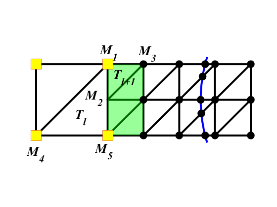
Figure 5.4. The green-painted area: Ωl−1,Γ∖ωl,Γ\Omega_{l-1,\Gamma}\setminus\omega_{l,\Gamma}.
Lemma 5.1.

For 0≤l≤L−10\leq l\leq L-1, it holds that

(5.8) ‖|(Πl+1−Πl)​v|‖0+hl​‖|(Πl+1−Πl)​v|‖1≲hl​‖|v|‖1∀v∈VL.{\left|\kern-1.07639pt\left|\kern-1.07639pt\left|(\Pi_{l+1}-\Pi_{l})v\right|\kern-1.07639pt\right|\kern-1.07639pt\right|}_{0}+h_{l}{\left|\kern-1.07639pt\left|\kern-1.07639pt\left|(\Pi_{l+1}-\Pi_{l})v\right|\kern-1.07639pt\right|\kern-1.07639pt\right|}_{1}\lesssim h_{l}{\left|\kern-1.07639pt\left|\kern-1.07639pt\left|v\right|\kern-1.07639pt\right|\kern-1.07639pt\right|}_{1}\quad\forall v\in V_{L}.
Proof.

By the definition of Πl\Pi_{l}, it has

(Πl+1−Πl)v={0,inωl,Γ,(Ql+1,β−Ql,β)​v,inΩ∖Ωl−1,Γ.\displaystyle(\Pi_{l+1}-\Pi_{l})v=\left\{\begin{aligned} &0,\penalty\ &\text{in}\penalty\ &\omega_{l,\Gamma},\\ &(Q_{l+1,\beta}-Q_{l,\beta})v,\penalty\ &\text{in}\penalty\ &\Omega\setminus\Omega_{l-1,\Gamma}.\end{aligned}\right.

Since

‖|(Ql+1,β−Ql,β)​v|‖0,Ω∖Ωl−1,Γ2+hl2​‖|(Ql+1,β−Ql,β)​v|‖1,Ω∖Ωl−1,Γ2≤∑j=ll+1(‖|v−Qj,β​v|‖0,Ω∖Ωl−1,Γ2+hl2​‖|v−Qj,β​v|‖1,Ω∖Ωl−1,Γ2)≲hl2​‖|v|‖12,\displaystyle\begin{aligned} &{\left|\kern-1.07639pt\left|\kern-1.07639pt\left|(Q_{l+1,\beta}-Q_{l,\beta})v\right|\kern-1.07639pt\right|\kern-1.07639pt\right|}_{0,\Omega\setminus\Omega_{l-1,\Gamma}}^{2}+h_{l}^{2}{\left|\kern-1.07639pt\left|\kern-1.07639pt\left|(Q_{l+1,\beta}-Q_{l,\beta})v\right|\kern-1.07639pt\right|\kern-1.07639pt\right|}_{1,\Omega\setminus\Omega_{l-1,\Gamma}}^{2}\\ &\leq\sum\limits_{j=l}^{l+1}({\left|\kern-1.07639pt\left|\kern-1.07639pt\left|v-Q_{j,\beta}v\right|\kern-1.07639pt\right|\kern-1.07639pt\right|}_{0,\Omega\setminus\Omega_{l-1,\Gamma}}^{2}+h_{l}^{2}{\left|\kern-1.07639pt\left|\kern-1.07639pt\left|v-Q_{j,\beta}v\right|\kern-1.07639pt\right|\kern-1.07639pt\right|}_{1,\Omega\setminus\Omega_{l-1,\Gamma}}^{2})\\ &\lesssim h_{l}^{2}{\left|\kern-1.07639pt\left|\kern-1.07639pt\left|v\right|\kern-1.07639pt\right|\kern-1.07639pt\right|}_{1}^{2},\end{aligned}

it only needs to estimate ‖|(Ql+1,β−Ql,β)​v|‖0,Ωl−1,Γ∖ωl,Γ{\left|\kern-1.07639pt\left|\kern-1.07639pt\left|(Q_{l+1,\beta}-Q_{l,\beta})v\right|\kern-1.07639pt\right|\kern-1.07639pt\right|}_{0,\Omega_{l-1,\Gamma}\setminus\omega_{l,\Gamma}}. Without loss of generality, assume Tl+1⊂Ωl−1,Γ∖ωl,ΓT_{l+1}\subset\Omega_{l-1,\Gamma}\setminus\omega_{l,\Gamma} as in Figure 5.4. It is obvious that Tl+1⊂Ω∖Ωl,ΓT_{l+1}\subset\Omega\setminus\Omega_{l,\Gamma}, therefore Πl+1​v|Tl+1=Ql+1,β​v\Pi_{l+1}v|_{T_{l+1}}=Q_{l+1,\beta}v. A direct calculation shows that

‖|(Πl+1−Πl)​v|‖0,Tl+12≲hl+12​∑1≤i≤2β⁡(M1)​(Ql+1,β​v​(Mi)−Ql,β​v​(Mi))2≲hl+1​β​(M1)​‖Ql+1,β​v−Ql,β​v‖0,M1​M22≲hl+1​β​(M1)​‖Ql+1,β​v−Ql,β​v‖0,M1​M52≲‖|Ql+1,β​v−Ql,β​v|‖0,Tl2+hl+12​‖|Ql+1,β​v−Ql,β​v|‖0,Tl2≲hl2​‖|v|‖1,Tl2.\displaystyle\begin{aligned} {\left|\kern-1.07639pt\left|\kern-1.07639pt\left|(\Pi_{l+1}-\Pi_{l})v\right|\kern-1.07639pt\right|\kern-1.07639pt\right|}_{0,T_{l+1}}^{2}&\lesssim h_{l+1}^{2}\sum_{1\leq i\leq 2}\beta(M_{1})(Q_{l+1,\beta}v(M_{i})-Q_{l,\beta}v(M_{i}))^{2}\\ &\lesssim h_{l+1}\beta(M_{1})\|Q_{l+1,\beta}v-Q_{l,\beta}v\|_{0,M_{1}M_{2}}^{2}\\ &\lesssim h_{l+1}\beta(M_{1})\|Q_{l+1,\beta}v-Q_{l,\beta}v\|_{0,M_{1}M_{5}}^{2}\\ &\lesssim{\left|\kern-1.07639pt\left|\kern-1.07639pt\left|Q_{l+1,\beta}v-Q_{l,\beta}v\right|\kern-1.07639pt\right|\kern-1.07639pt\right|}_{0,T_{l}}^{2}+h_{l+1}^{2}{\left|\kern-1.07639pt\left|\kern-1.07639pt\left|Q_{l+1,\beta}v-Q_{l,\beta}v\right|\kern-1.07639pt\right|\kern-1.07639pt\right|}_{0,T_{l}}^{2}\\ &\lesssim h_{l}^{2}{\left|\kern-1.07639pt\left|\kern-1.07639pt\left|v\right|\kern-1.07639pt\right|\kern-1.07639pt\right|}_{1,T_{l}}^{2}.\end{aligned}

Similarly, it is easy to derive that ‖|(Πl+1−Πl)​v|‖1,Tl+12≲‖|v|‖1,Tl2{\left|\kern-1.07639pt\left|\kern-1.07639pt\left|(\Pi_{l+1}-\Pi_{l})v\right|\kern-1.07639pt\right|\kern-1.07639pt\right|}_{1,T_{l+1}}^{2}\lesssim{\left|\kern-1.07639pt\left|\kern-1.07639pt\left|v\right|\kern-1.07639pt\right|\kern-1.07639pt\right|}_{1,T_{l}}^{2}. Summing Tl+1T_{l+1} over Ωl,Γ∖ωl,Γ\Omega_{l,\Gamma}\setminus\omega_{l,\Gamma}, it yields

‖|(Πl+1−Πl)​v|‖0,Ωl−1,Γ∖ωl,Γ2+hl2​‖|(Πl+1−Πl)​v|‖1,Ωl−1,Γ∖ωl,Γ2≲hl2​‖|v|‖12.{\left|\kern-1.07639pt\left|\kern-1.07639pt\left|(\Pi_{l+1}-\Pi_{l})v\right|\kern-1.07639pt\right|\kern-1.07639pt\right|}_{0,\Omega_{l-1,\Gamma}\setminus\omega_{l,\Gamma}}^{2}+h_{l}^{2}{\left|\kern-1.07639pt\left|\kern-1.07639pt\left|(\Pi_{l+1}-\Pi_{l})v\right|\kern-1.07639pt\right|\kern-1.07639pt\right|}_{1,\Omega_{l-1,\Gamma}\setminus\omega_{l,\Gamma}}^{2}\lesssim h_{l}^{2}{\left|\kern-1.07639pt\left|\kern-1.07639pt\left|v\right|\kern-1.07639pt\right|\kern-1.07639pt\right|}_{1}^{2}.

This completes the proof. ∎

Lemma 5.2.

For 0≤l≤L0\leq l\leq L, it holds

(5.9) ‖|v−Πl​v|‖0+hl​‖|v−Πl​v|‖1≤C​hl​‖|v|‖1∀v∈VL.{\left|\kern-1.07639pt\left|\kern-1.07639pt\left|v-\Pi_{l}v\right|\kern-1.07639pt\right|\kern-1.07639pt\right|}_{0}+h_{l}{\left|\kern-1.07639pt\left|\kern-1.07639pt\left|v-\Pi_{l}v\right|\kern-1.07639pt\right|\kern-1.07639pt\right|}_{1}\leq Ch_{l}{\left|\kern-1.07639pt\left|\kern-1.07639pt\left|v\right|\kern-1.07639pt\right|\kern-1.07639pt\right|}_{1}\quad\forall v\in V_{L}.
Proof.

By Lemma 5.1 and the triangle inequality, it’s easy to derive that

‖|v−Πl​v|‖0+hl​‖|v−Πl​v|‖1≤∑r=lL−1(‖|πr+1​v−Πr​v|‖0+hr​‖|Πr+1​v−Πr​v|‖1)≲hl​‖|v|‖1.\displaystyle\begin{aligned} &{\left|\kern-1.07639pt\left|\kern-1.07639pt\left|v-\Pi_{l}v\right|\kern-1.07639pt\right|\kern-1.07639pt\right|}_{0}+h_{l}{\left|\kern-1.07639pt\left|\kern-1.07639pt\left|v-\Pi_{l}v\right|\kern-1.07639pt\right|\kern-1.07639pt\right|}_{1}\\ &\leq\sum\limits_{r=l}^{L-1}({\left|\kern-1.07639pt\left|\kern-1.07639pt\left|\pi_{r+1}v-\Pi_{r}v\right|\kern-1.07639pt\right|\kern-1.07639pt\right|}_{0}+h_{r}{\left|\kern-1.07639pt\left|\kern-1.07639pt\left|\Pi_{r+1}v-\Pi_{r}v\right|\kern-1.07639pt\right|\kern-1.07639pt\right|}_{1})\\ &\lesssim h_{l}{\left|\kern-1.07639pt\left|\kern-1.07639pt\left|v\right|\kern-1.07639pt\right|\kern-1.07639pt\right|}_{1}.\end{aligned}

∎

According to the space decomposition (5.3), for any v∈VLv\in V_{L}, do the following decomposition

(5.10) v=v0+∑l=1L(vl,0+∑i=1nl,ωvl,i),\displaystyle v=v_{0}+\sum_{l=1}^{L}(v_{l,0}+\sum\limits_{i=1}^{n_{l,\omega}}v_{l,i}),

where v0=Π0​v∈V0v_{0}=\Pi_{0}v\in V_{0}, and vl,i=πl​((Πl​v−Πl−1​v)​ϕl,i)∈Vl,iv_{l,i}=\pi_{l}((\Pi_{l}v-\Pi_{l-1}v)\phi_{l,i})\in V_{l,i} for i=0,1,⋯,nl,ωi=0,1,\cdots,n_{l,\omega}.

Lemma 5.3.

The V-cycle algorithm (2) has the following convergence rate estimate

(5.11) ‖I−BL​AL‖AL≤1−11+C​|log⁡hL|.\|I-B_{L}A_{L}\|_{A_{L}}\leq 1-\frac{1}{1+C|\log h_{L}|}.

The proof included below mainly follows [22], specific details are still given for completeness.

Proof.

By X-Z identity (see [23]), it holds

‖I−BL​AL‖AL≤1−11+c0,\|I-B_{L}A_{L}\|_{A_{L}}\leq 1-\frac{1}{1+c_{0}},

with

c0=sup‖|v|‖1=1infv=v0+∑l=1L∑i=0nl,ωvl,ic⁡(v),c_{0}=\sup_{{\left|\kern-0.75346pt\left|\kern-0.75346pt\left|v\right|\kern-0.75346pt\right|\kern-0.75346pt\right|}_{1}=1}\inf_{v=v_{0}+\sum_{l=1}^{L}\sum\limits_{i=0}^{n_{l,\omega}}v_{l,i}}c(v),

where

c⁡(v)=‖|P0​(v−v0)|‖12+∑l=1L∑i=0nl,ω‖|Pl,i​∑(k,j)>(l,i)vk,j|‖12.c(v)={\left|\kern-1.07639pt\left|\kern-1.07639pt\left|P_{0}(v-v_{0})\right|\kern-1.07639pt\right|\kern-1.07639pt\right|}_{1}^{2}+\sum\limits_{l=1}^{L}\sum_{i=0}^{n_{l,\omega}}{\left|\kern-1.07639pt\left|\kern-1.07639pt\left|P_{l,i}\sum_{(k,j)>(l,i)}v_{k,j}\right|\kern-1.07639pt\right|\kern-1.07639pt\right|}_{1}^{2}.

Let Δl,i=s​u​p​p​(ϕl,i)\Delta_{l,i}=supp(\phi_{l,i}) and notice

∑(k,j)>(l,i)vk,j=(v−Πl​v)+∑j=i+1nl,ωvl,j,\sum_{(k,j)>(l,i)}v_{k,j}=(v-\Pi_{l}v)+\sum\limits_{j=i+1}^{n_{l,\omega}}v_{l,j},
∑l=1L∑i=0nl,ω‖|Pl,i​∑(k,j)>(l,i)vk,j|‖12≲∑l=1L∑i=0nl,ω(‖|Pl,i​(v−Πl​v)|‖12+‖|Pl,i​∑j=i+1nl,ωvl,j|‖12)≲∑l=1L∑i=0nl,ω(‖|v−Πl​v|‖1,Δl,i2+∑j=i+1nl,ω‖|vl,j|‖1,Δl,i2).\displaystyle\begin{aligned} \sum\limits_{l=1}^{L}\sum_{i=0}^{n_{l,\omega}}{\left|\kern-1.07639pt\left|\kern-1.07639pt\left|P_{l,i}\sum_{(k,j)>(l,i)}v_{k,j}\right|\kern-1.07639pt\right|\kern-1.07639pt\right|}_{1}^{2}&\lesssim\sum\limits_{l=1}^{L}\sum_{i=0}^{n_{l,\omega}}({\left|\kern-1.07639pt\left|\kern-1.07639pt\left|P_{l,i}(v-\Pi_{l}v)\right|\kern-1.07639pt\right|\kern-1.07639pt\right|}_{1}^{2}+{\left|\kern-1.07639pt\left|\kern-1.07639pt\left|P_{l,i}\sum_{j=i+1}^{n_{l,\omega}}v_{l,j}\right|\kern-1.07639pt\right|\kern-1.07639pt\right|}_{1}^{2})\\ &\lesssim\sum\limits_{l=1}^{L}\sum_{i=0}^{n_{l,\omega}}({\left|\kern-1.07639pt\left|\kern-1.07639pt\left|v-\Pi_{l}v\right|\kern-1.07639pt\right|\kern-1.07639pt\right|}_{1,\Delta_{l,i}}^{2}+\sum_{j=i+1}^{n_{l,\omega}}{\left|\kern-1.07639pt\left|\kern-1.07639pt\left|v_{l,j}\right|\kern-1.07639pt\right|\kern-1.07639pt\right|}_{1,\Delta_{l,i}}^{2}).\end{aligned}

Observe that

∑l=1L∑i=0nl,ω‖|v−Πl​v|‖1,Δl,i2=∑l=1L‖|v−Πl​v|‖1,Ω2≲|log⁡hL|​‖|v|‖1,Ω2,\sum\limits_{l=1}^{L}\sum_{i=0}^{n_{l,\omega}}{\left|\kern-1.07639pt\left|\kern-1.07639pt\left|v-\Pi_{l}v\right|\kern-1.07639pt\right|\kern-1.07639pt\right|}_{1,\Delta_{l,i}}^{2}=\sum\limits_{l=1}^{L}{\left|\kern-1.07639pt\left|\kern-1.07639pt\left|v-\Pi_{l}v\right|\kern-1.07639pt\right|\kern-1.07639pt\right|}_{1,\Omega}^{2}\lesssim|\log h_{L}|{\left|\kern-1.07639pt\left|\kern-1.07639pt\left|v\right|\kern-1.07639pt\right|\kern-1.07639pt\right|}_{1,\Omega}^{2},

and

∑l=1L∑i=0nl,ω∑j=i+1nl,ω‖|vl,j|‖1,Δl,i2≲∑l=1L(‖|vl,0|‖1,Δl,02+∑i=1nl,ω∑j=i+1nl,ωhl−2​‖|vl,j|‖0,Δl,i2)≲∑l=1L(‖|πl​((Πl​v−Πl−1​v)​ϕl,0)|‖1,Δl,02+∑i=1nl,ω∑j=i+1nl,ωhl−2​‖|vl,j|‖0,Δl,i2)≲∑l=1L(‖|Πl​v−Πl−1​v|‖1,Δl,02+∑i=0nl,ωhl−2​‖|Πl​v−Πl−1​v|‖0,Δl,i2)≲|log⁡hL|​‖|v|‖12.\displaystyle\begin{aligned} \sum\limits_{l=1}^{L}\sum_{i=0}^{n_{l,\omega}}\sum_{j=i+1}^{n_{l,\omega}}{\left|\kern-1.07639pt\left|\kern-1.07639pt\left|v_{l,j}\right|\kern-1.07639pt\right|\kern-1.07639pt\right|}_{1,\Delta_{l,i}}^{2}&\lesssim\sum\limits_{l=1}^{L}({\left|\kern-1.07639pt\left|\kern-1.07639pt\left|v_{l,0}\right|\kern-1.07639pt\right|\kern-1.07639pt\right|}_{1,\Delta_{l,0}}^{2}+\sum_{i=1}^{n_{l,\omega}}\sum_{j=i+1}^{n_{l,\omega}}h_{l}^{-2}{\left|\kern-1.07639pt\left|\kern-1.07639pt\left|v_{l,j}\right|\kern-1.07639pt\right|\kern-1.07639pt\right|}_{0,\Delta_{l,i}}^{2})\\ &\lesssim\sum\limits_{l=1}^{L}({\left|\kern-1.07639pt\left|\kern-1.07639pt\left|\pi_{l}((\Pi_{l}v-\Pi_{l-1}v)\phi_{l,0})\right|\kern-1.07639pt\right|\kern-1.07639pt\right|}_{1,\Delta_{l,0}}^{2}+\sum_{i=1}^{n_{l,\omega}}\sum_{j=i+1}^{n_{l,\omega}}h_{l}^{-2}{\left|\kern-1.07639pt\left|\kern-1.07639pt\left|v_{l,j}\right|\kern-1.07639pt\right|\kern-1.07639pt\right|}_{0,\Delta_{l,i}}^{2})\\ &\lesssim\sum\limits_{l=1}^{L}({\left|\kern-1.07639pt\left|\kern-1.07639pt\left|\Pi_{l}v-\Pi_{l-1}v\right|\kern-1.07639pt\right|\kern-1.07639pt\right|}_{1,\Delta_{l,0}}^{2}+\sum_{i=0}^{n_{l,\omega}}h_{l}^{-2}{\left|\kern-1.07639pt\left|\kern-1.07639pt\left|\Pi_{l}v-\Pi_{l-1}v\right|\kern-1.07639pt\right|\kern-1.07639pt\right|}_{0,\Delta_{l,i}}^{2})\\ &\lesssim|\log h_{L}|{\left|\kern-1.07639pt\left|\kern-1.07639pt\left|v\right|\kern-1.07639pt\right|\kern-1.07639pt\right|}_{1}^{2}.\end{aligned}

Combining the above inequalities concludes the proof. ∎

6. Numerical Examples

In this section, we present several numerical examples to show the performance of our methods. Particular attention will be paid on verifying its high order convergence and examining its robustness in dealing with low regularity solutions and complex geometries. The computational domain is the rectangle −1≤x,y≤1-1\leq x,y\leq 1, and the interface is denoted by a levelset function ϕ⁡(x,y)\phi(x,y), i.e.,

Ω={(x,y)∈ℝ2;−1≤x,y≤1},\displaystyle\Omega=\{(x,y)\in\mathbb{R}^{2};-1\leq x,y\leq 1\},
Ω1={(x,y)∈Ω;ϕ⁡(x,y)>0},\displaystyle\Omega_{1}=\{(x,y)\in\Omega;\phi(x,y)>0\},
Ω2={(x,y)∈Ω;ϕ⁡(x,y)<0}.\displaystyle\Omega_{2}=\{(x,y)\in\Omega;\phi(x,y)<0\}.

We test the multigrid algorithm 2 with these examples, the initial guess is 𝟎\bm{0}, and the stopping criterion is the l2l^{2} norm of the relative residual being smaller than exp(-20).

6.1. Example 1

The interface is a circle centered at the origin with radius rr, i.e.,

ϕ⁡(x,y)=x2+y2−r2.\phi(x,y)=x^{2}+y^{2}-r^{2}.

The exact solution is chosen as follows

u=1β​ϕ​(x,y)​sin⁡(π​x)​sin⁡(π​y).u=\frac{1}{\beta}\phi(x,y)\sin(\pi x)\sin(\pi y).

We test the local anisotropic FEM for the second order elliptic interface problem (1.1) whose exact solutions are defined as above and whose coefficient jump ratio β1/β2=104,102,10−2,10−4\beta_{1}/\beta_{2}=10^{4},10^{2},10^{-2},10^{-4}. Numerical results are shown in Tables 6.1-6.1, illustrating that the convergence rates are optimal in H1H^{1}-norm and L2L^{2}-norm. Figure 6.1 illustrates that our method allows discontinuity of the gradient of the solution uu on the interface.

Table 6.1. Finite element errors for Example 1 with β1=104\beta_{1}=10^{4}, β2=1\beta_{2}=1.
1h\frac{1}{h} ‖u−uh‖0,Ω\|u-u_{h}\|_{0,\Omega} order |u−uh|1,Ω|u-u_{h}|_{1,\Omega} order
32 1.3399e-03 3.3520e-02
64 3.6122e-04 1.8911 1.7466e-02 0.9404
128 9.0503e-05 1.9968 8.8375e-03 0.9828
256 2.2666e-05 1.9974 4.4497e-03 0.9899
512 5.6388e-06 2.0070 2.2724e-03 0.9694
Table 6.2. Finite element errors for Example 1 with β1=102\beta_{1}=10^{2}, β2=1\beta_{2}=1.
1h\frac{1}{h} ‖u−uh‖0,Ω\|u-u_{h}\|_{0,\Omega} order |u−uh|1,Ω|u-u_{h}|_{1,\Omega} order
32 1.3415e-03 3.3523e-02
64 3.6107e-04 1.8935 1.7467e-02 0.9404
128 9.0456e-05 1.9969 8.8399e-03 0.9825
256 2.2638e-05 1.9984 4.4511e-03 0.9898
512 5.6057e-06 2.0138 2.2727e-03 0.9697
Table 6.3. Finite element errors for Example 1 with β1=1\beta_{1}=1, β2=102\beta_{2}=10^{2}.
1h\frac{1}{h} ‖u−uh‖0,Ω\|u-u_{h}\|_{0,\Omega} order |u−uh|1,Ω|u-u_{h}|_{1,\Omega} order
32 3.9442e-03 9.7003e-02
64 9.9666e-04 1.9845 4.8823e-02 0.9904
128 2.5030e-04 1.9934 2.4450e-02 0.9977
256 6.2653e-05 1.9982 1.2252e-02 0.9967
512 1.5648e-05 2.0013 6.1377e-03 0.9973
Table 6.4. Finite element errors for Example 1 with β1=1\beta_{1}=1, β2=104\beta_{2}=10^{4}.
1h\frac{1}{h} ‖u−uh‖0,Ω\|u-u_{h}\|_{0,\Omega} order |u−uh|1,Ω|u-u_{h}|_{1,\Omega} order
32 3.9444e-03 9.7007e-02
64 9.9671e-04 1.9845 4.8825e-02 0.9904
128 2.5033e-04 1.9933 2.4450e-02 0.9977
256 6.2665e-05 1.9981 1.2253e-02 0.9967
512 1.5659e-05 2.0006 6.1379e-03 0.9973

From Tables 6.1-6.1, we can see that the desired multigrid method converges uniformly with respect to the mesh size and the jump ratio.

Table 6.5. Numerical performance of Algorithm 2 for Example 1 with β1/β2=10−4\beta_{1}/\beta_{2}=10^{-4}.
hh 2−62^{-6} 2−72^{-7} 2−82^{-8} 2−92^{-9}
#\#iter 8 8 8 8
Table 6.6. Numerical performance of Algorithm 2 for Example 1 with h=2−9h=2^{-9}.
β1/β2\beta_{1}/\beta_{2} 10410^{4} 10210^{2} 10−210^{-2} 10−410^{-4}
#\#iter 8 8 8 8
Refer to caption
Refer to caption
Figure 6.1. Numerical solutions for Example 1 with β1/β2=104\beta_{1}/\beta_{2}=10^{4}(left) and β1/β2=10−4\beta_{1}/\beta_{2}=10^{-4}(right).

6.2. Example 2

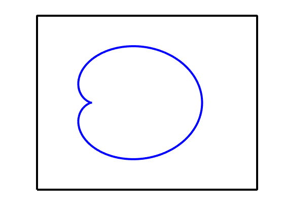
The interface is a cardioid curve (see Figure 6.2),
ϕ⁡(x,y)=((x+0.5)2+y2−0.5​(x+0.5))2−0.25​((x+0.5)2+y2).\phi(x,y)=((x+0.5)^{2}+y^{2}-0.5(x+0.5))^{2}-0.25((x+0.5)^{2}+y^{2}).
Refer to caption
Figure 6.2. A cardioid interface.

Then the exact solution is chosen as follows

u=1β​sin⁡(π​x)​sin⁡(π​y)+5​δ​(x,y),u=\frac{1}{\beta}\sin(\pi x)\sin(\pi y)+5\delta(x,y),

where

δ(x,y)={0,(x,y)∈Ω1,1,(x,y)∈Ω2.\displaystyle\delta(x,y)=\left\{\begin{aligned} &0,\penalty\ \penalty\ (x,y)\in\Omega_{1},\\ &1,\penalty\ \penalty\ (x,y)\in\Omega_{2}.\end{aligned}\right.

We test our method for the second order elliptic interface problem (1.1) whose exact solutions are defined as above and whose coefficient jump ratio β1/β2=103,10−3\beta_{1}/\beta_{2}=10^{3},10^{-3}, Numerical results are shown in Figure 6.6, illustrating that the convergence rates are optimal in H1H^{1}-norm and L2L^{2}-norm. For the non-homogeneous case, Table 6.2-6.2 show that our multigrid algorithm is still optimal.

Refer to caption
Refer to caption
Figure 6.3. Finite element error analysis in log-log scale for Example 2 with β1/β2=103\beta_{1}/\beta_{2}=10^{3}(left) and β1/β2=10−3\beta_{1}/\beta_{2}=10^{-3}(right).
Refer to caption
Refer to caption
Figure 6.4. Numerical solutions for Example 2 with β1/β2=103\beta_{1}/\beta_{2}=10^{3}(left) and β1/β2=10−3\beta_{1}/\beta_{2}=10^{-3}(right).
Table 6.7. Numerical performance of Algorithm 2 for Example 2 with β1/β2=10−4\beta_{1}/\beta_{2}=10^{-4}.
hh 2−62^{-6} 2−72^{-7} 2−82^{-8} 2−92^{-9}
#\#iter 9 9 9 9
Table 6.8. Numerical performance of Algorithm 2 for Example 2 with h=2−9h=2^{-9}.
β1/β2\beta_{1}/\beta_{2} 10410^{4} 10210^{2} 10−210^{-2} 10−410^{-4}
#\#iter 9 9 9 9

6.3. Example 3

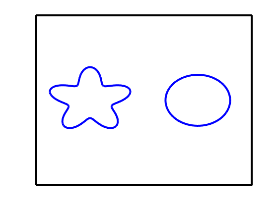
There are two interfaces in this example, one is a five star curve, the other is a circle ( see Figure 6.5), i.e,

ϕ⁡(x,y)=(ρ1−0.3−0.09​sin⁡(5​θ))​(ρ22−0.09),\phi(x,y)=(\rho_{1}-0.3-0.09\sin(5\theta))(\rho_{2}^{2}-0.09),

where ρ1=(x+0.5)2+y2\rho_{1}=(x+0.5)^{2}+y^{2}, ρ2=(x−0.5)2+y2\rho_{2}=(x-0.5)^{2}+y^{2}. The exact solution is chosen as follows

u=1β​sin⁡(π​x)​sin⁡(π​y)+δ⁡(x,y).u=\frac{1}{\beta}\sin(\pi x)\sin(\pi y)+\delta(x,y).

We test the local anisotropic FEM for the second order elliptic interface problem (1.1) whose exact solutions are defined as above and whose coefficient jump ratio β1/β2=103,10−3\beta_{1}/\beta_{2}=10^{3},10^{-3}. Numerical results are shown in Figure 6.6, illustrating that the convergence rates are optimal in H1H^{1}-norm and L2L^{2}-norm.

Refer to caption
Figure 6.5. A five star and a circle interfaces.
Refer to caption
Refer to caption
Figure 6.6. Finite element error analysis in log-log scale for Example 3 with β1/β2=103\beta_{1}/\beta_{2}=10^{3}(left) and β1/β2=10−3\beta_{1}/\beta_{2}=10^{-3}(right).
Refer to caption
Refer to caption
Figure 6.7. Numerical solutions for Example 3 with β1/β2=103\beta_{1}/\beta_{2}=10^{3}(left) and β1/β2=10−3\beta_{1}/\beta_{2}=10^{-3}(right).

Still Table 6.2-6.2 show that our multigrid algorithm has an optimal convergence rate independent of the mesh size and jump ratio.

Table 6.9. Numerical performance of Algorithm 2 for Example 3 with β1/β2=10−4\beta_{1}/\beta_{2}=10^{-4}.
hh 2−62^{-6} 2−72^{-7} 2−82^{-8} 2−92^{-9}
#\#iter 8 8 8 8
Table 6.10. Numerical performance of Algorithm 2 for Example 3 with h=2−9h=2^{-9}.
β1/β2\beta_{1}/\beta_{2} 10410^{4} 10210^{2} 10−210^{-2} 10−410^{-4}
#\#iter 8 8 8 8

References

  • [1] G. Acosta and R. G. Duran. Error estimates for Q1Q_{1} isoparametric elements satisfying a weak angle condition. SIAM Journal on Numerical Analysis, 38:1073–1088, 2000.
  • [2] R. A. Adams and J. J. Fournier. Sobolev Spaces. Academic press, 2003.
  • [3] S. Adjerid, N. Chaabane, and T. Lin. An immersed discontinuous finite element method for Stokes interface problems. Computer Methods in Applied Mechanics and Engineering, 293:170–190, 2015.
  • [4] I. Babuška. The finite element method for elliptic equations with discontinuous coefficients. Computing, 5:207–213, 1970.
  • [5] I. Babuška and A. K. Aziz. On the angle condition in the finite element method. SIAM Journal on Numerical Analysis, 13:214–226, 1976.
  • [6] T. Belytschko and T. Black. Elastic crack growth in finite elements with minimal remeshing. International Journal for Numerical Methods in Engineering, 45:601–620, 1999.
  • [7] J. H. Bramble and J. T. King. A finite element method for interface problems in domains with smooth boundaries and interfaces. Advances in Computational Mathematics, 6:109–138, 1996.
  • [8] E. Burman, J. Guzmán, M. A. Sánchez, and M. Sarkis. Robust flux error estimation of an unfitted Nitsche method for high-contrast interface problems. IMA Journal of Numerical Analysis, 2016.
  • [9] L. Chen, H. Wei, and M. Wen. An interface-fitted mesh generator and virtual element methods for elliptic interface problems. Journal of Computational Physics, 334:327–348, 2017.
  • [10] Z. Chen and J. Zou. Finite element methods and their convergence for elliptic and parabolic interface problems. Numerische Mathematik, 79:175–202, 1998.
  • [11] J. Guzmán, M. Sánchez, and M. Sarkis. On the accuracy of finite element approximations to a class of interface problems. Mathematics of Computation, 85(301):2071–2098, 2016.
  • [12] A. Hansbo and P. Hansbo. An unfitted finite element method, based on Nitsche’s method, for elliptic interface problems. Computer Methods in Applied Mechanics and Engineering, 191:5537–5552, 2002.
  • [13] A. Hansbo and P. Hansbo. A finite element method for the simulation of strong and weak discontinuities in solid mechanics. Computer Methods in Applied Mechanics and Engineering, 193:3523–3540, 2004.
  • [14] P. Hansbo, M. G. Larson, and S. Zahedi. A cut finite element method for a Stokes interface problem. Applied Numerical Mathematics, 85:90–114, 2014.
  • [15] J. Huang and J. Zou. Some new a priori estimates for second order elliptic and parabolic interface problems. Journal of Differential Equations, 184:570–586, 2002.
  • [16] J. Huang and J. Zou. Uniform a priori estimates for elliptic and static Maxwell interface problems. Discrete and Continuous Dynamicals Systems-Series B, 7:145–170, 2007.
  • [17] K. Kergrene, I. Babuška, and U. Banerjee. Stable generalized finite element method and associated iterative schemes; application to interface problems. Computer Methods in Applied Mechanics and Engineering, 305:1–36, 2016.
  • [18] Z. Li. The immersed interface method using a finite element formulation. Applied Numerical Mathematics, 27:253–267, 1998.
  • [19] Z. Li, T. Lin, and X. Wu. New Cartesian grid methods for interface problems using the finite element formulation. Numerische Mathematik, 96:61–98, 2003.
  • [20] J. Xu. Estimate of the convergence rate of finite element solutions to elliptic equations of second order with discontinuous coefficients. Natural Science Journal of Xiangtan University (in Chinese), 1:84–88, 1982.
  • [21] J. Xu and S. Zhang. Optimal finite element methods for interface problems. Domain Decomposition Methods in Science and Engineering XXII, pages 77–91, 2016.
  • [22] J. Xu and Y. Zhu. Uniform convergent multigrid methods for elliptic problems with strongly discontinuous coefficients. Mathematical Models and Methods in Applied Sciences, 18:77–105, 2008.
  • [23] J. Xu and L. Zikatanov. The method of alternating projections and the method of subspace corrections in Hilbert space. Journal of the American Mathematical Society, 15:573–597, 2002.
  • [24] G. Zi and T. Belytschko. New crack-tip elements for XFEM and applications to cohesive cracks. International Journal for Numerical Methods in Engineering, 57:2221–2240, 2003.