MPC-based Vibration Control and Energy Harvesting Using an Electromagnetic Vibration Absorber With Inertia Nonlinearity

Fig. 1 shows the schematic of the proposed electromagnetic vibration absorber with inertia nonlinearity. The key component of the absorber is the rotary electromagnetic generator that passively changes its moment of inertia. The passive change of moment of inertia is achieved by connecting the rotor of the electromagnetic generator with a sliding mass that is constrained to move along a motion guide fixed to the housing via a slotted rod that allows the mass to move relatively in the radial direction. Meanwhile, the angular motion of the mass and the rotor are identical. Because the radial position of the mass depends on its angular position, the moment of inertia of the rotor-mass system is a function of the angular position. Depending on the design of the motion guide, the moment of inertia can increase or decrease as the angular position changes. The working principle of the absorber is briefly explained as follows. When the two terminals are connected to a vehicle body and its suspension strut, respectively, the vibration of the vehicle translates the nut back and forth, subsequently rotating the screw. Because the rotor of the generator is attached to the screw via the torsion spring, it oscillates relative to the screw. As a result, some of the vibration energy is transferred to the kinetic energy of the oscillating rotor-mass system. In principle, the more kinetic energy transferred, the better the vibration suppression can be achieved. Because the kinetic energy is proportional to the moment of inertia of the absorber, one shall design a motion guide such that the moment of inertia increases as the angular position increases. Therefore, in this paper, a motion guide that enables “enlarging inertia” is used.

Furthermore, the absorbed kinetic energy is converted into electricity by the electromagnetic generator to achieve energy regeneration. The rate of energy regeneration can be controlled by the duty cycle of the generator; see Fig. 2. As a result, an energy regeneration circuit can be idealized as pure resistance shunt [21]. In many practical scenarios, the impedance of inductance of a generator is negligible when compared with the impedance of the energy regeneration circuit [35]. As such, the energy regeneration circuit can be modeled as an ideal viscous damper. By controlling the duty cycle, the damping force of the device can be controlled semi-actively.

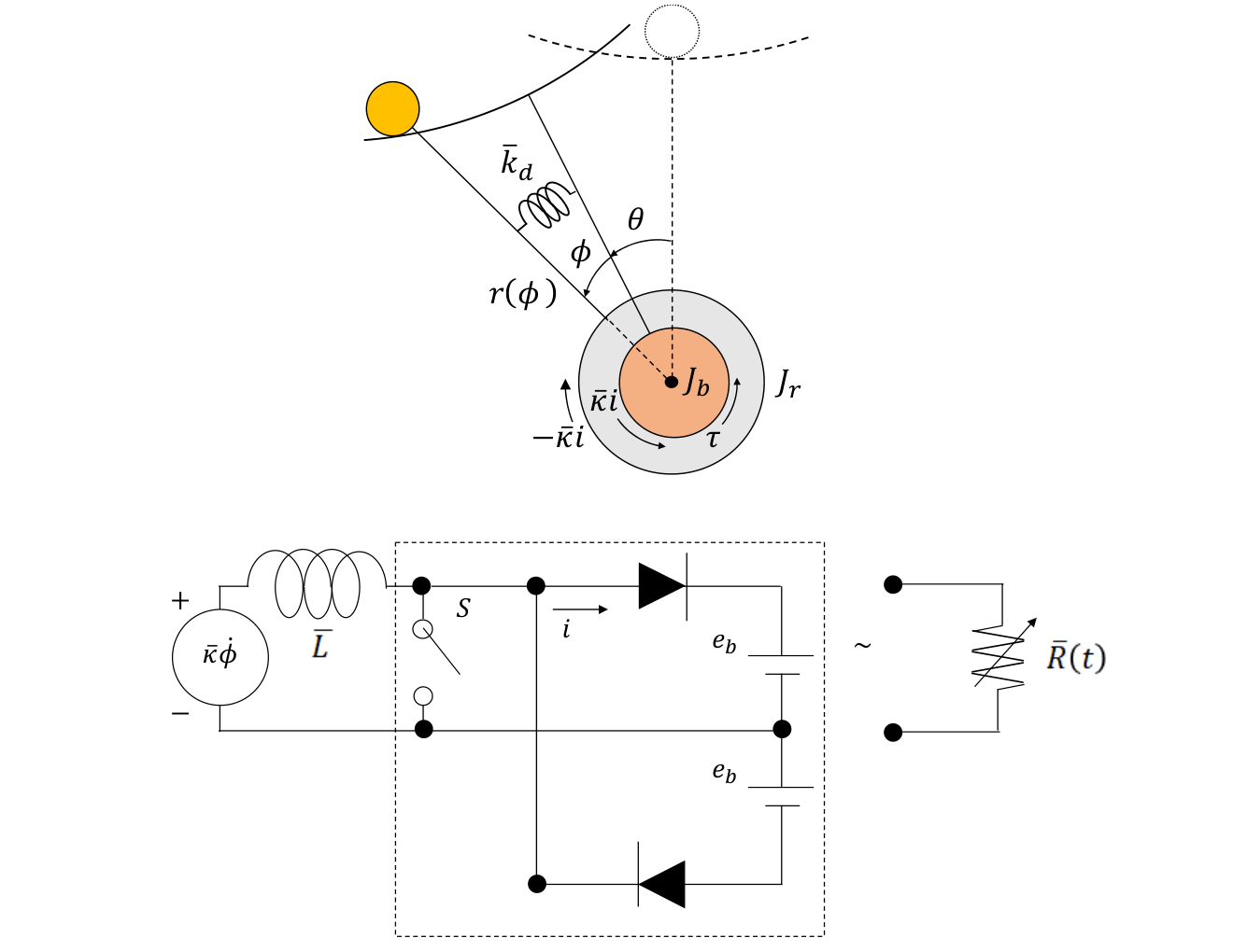
Fig. 2 shows a mathematical model of the absorber. Lagrange’s equation is used to derive the equations of motion of the system. Suppose the angular position of the motion guide and the angular position of the mass relative to the motion guide are $\theta$ and $\phi$, respectively. The radial position of the mass depends on the relative angular position and is written as $r=r\left(\phi\right)$. When using the polar coordinates, the kinetic energy of the system is written as,

$$T=\frac{m}{2}\left[\left(r^{\prime}\dot{\phi}\right)^{2}+r^{2}\left(\dot{\phi}+\dot{\theta}\right)^{2}\right]+\frac{J_{r}}{2}\left(\dot{\phi}+\dot{\theta}\right)^{2}+\frac{J_{b}}{2}\dot{\theta}^{2}$$

(1)

where $r^{\prime}=dr/d\phi$ and $m$ is the mass, and $J_{r}$, $J_{b}$ are the moment of inertia of the rotor and of the ball screw (including the housing), respectively. Furthermore, the potential energy is,

$$V=\frac{\bar{k}_{d}}{2}\phi^{2}$$

(2)

where $\bar{k}_{d}$ is the stiffness of the torsion spring. When a pair of parallel forces of equal magnitude $F(\gg mg)$ is applied to the two terminals in opposite directions, the screw is subject to a torque $\tau=lF$, where $l$ represents the effective moment arm, which depends on the parameters of the ball screw, e.g., the screw pitch. The virtual work done by the torques is,

$$\delta W_{\theta}=Q_{\theta}\delta\theta=\tau\delta\theta$$

(3)

where $Q_{\theta}$ is the corresponding generalized force. The rotor and the ball screw are subject to a pair of resistance torques of equal magnitude and opposite directions due to the back electromotive force (emf). The torque on the rotor $-\bar{\kappa}i$ is proportional to the current $i$, where $\bar{\kappa}$ is the torque constant. The torque on the ball screw is then obtained by removing the negative sign. The energy harvesting circuit can be idealized as a variable resistance $R(t)$ that takes away the electrical energy. The virtual work done by the resistance torque is written as,

$$\delta W=Q\delta\phi=-\bar{\kappa}i\delta\phi$$

(4)

and the electrical virtual work done on a charge by the electrical field across the resistor is,

$$\delta W_{R}=Q_{R}\delta q=-R(t)i\delta q$$

(5)

where $q$ is the electrical charge, and the electrical work done by the emf is,

$$\delta W_{e}=Q_{e}\delta q=\bar{\kappa}\dot{\phi}\delta q$$

(6)

where $Q$, $Q_{R}$, and $Q_{e}$ are the generalized forces. Furthermore, the energy stored in the inductance is,

$$E=\frac{1}{2}Li^{2}$$

(7)

The Lagrange equations are derived as,

$$\frac{d}{dt}\frac{\partial L}{\partial\dot{g}_{i}}-\frac{\partial L}{\partial g_{i}}=Q_{i}$$

(8)

where $L=T+E-V$ is the Lagrangian, $g_{1}=\phi$, $g_{2}=\theta$, and $g_{3}=q$ are the generalized coordinates, and $Q_{1}=Q$, $Q_{2}=Q_{\theta}$, and $Q_{3}=Q_{R}+Q_{e}$. After substituting (1) to (7) into (8), using the angular position of the rotor $\psi=\phi+\theta$, and idealizing the electrical circuit as pure resistance shunt, the equations of motion are derived as,

		$\displaystyle\left(J_{r}+J_{eff}\right)\ddot{\psi}+mr_{eff}\dot{\psi}^{2}-2mr_{eff}\dot{\theta}\dot{\psi}+mr^{\prime}r^{\prime\prime}\dot{\theta}^{2}$		(9)
		$\displaystyle-m\left(r^{\prime}\right)^{2}\ddot{\theta}+\bar{k}_{d}\left(\psi-\theta\right)+c_{e}(t)\left(\dot{\psi}-\dot{\theta}\right)=0$

$$J_{b}\ddot{\theta}+2mrr^{\prime}\left(\dot{\psi}^{2}-\dot{\psi}\dot{\theta}\right)+\left(J_{r}+mr^{2}\right)\ddot{\psi}=Fl$$

(10)

where $J_{eff}=m\left[r^{2}+\left(r^{\prime}\right)^{2}\right]$ is the effective moment of inertia of the mass, $r_{eff}=\left(rr^{\prime}+r^{\prime}r^{\prime\prime}\right)$ is the effective radius, $r^{\prime\prime}=d^{2}r/d\phi^{2}$, and $c_{e}(t)=\bar{\kappa}^{2}/R(t)$ is the semi-actively controlled electrical damping coefficient. For the rest of the paper, the radial position $r(\phi)=r(0)+\lambda r_{1}(\phi)=r_{0}+\lambda r_{1}(\phi)$ is considered, where $\lambda$ is a length constant.

The superior performance of this new design will be demonstrated in the numerical simulations in Section VI.A.

In this section, a nonlinear Model Predictive Controller (NMPC) is implemented for ERVA control. The system dynamics is based on the the quarter-car model as shown in Fig. 3. Here $M_{s}$ and $M_{us}$ are sprung mass and unsprung mass, respectively; $z_{s}$ and $z_{us}$ are the corresponding displacements, $z_{r}$ is the road profile; $k_{s}$ and $k_{t}$ are, respectively, spring stiffness and tire stiffness, and $c$ is the damper coefficient. The ERVA is mounted between the sprung mass and unsprung mass, reacting by the applied force $F$. By the analysis of Newton’s second law on this model, the equations of motion (EOM) of this quarter car, together with ERVA are derived in the differential equation form as,

		$\displaystyle M_{s}\ddot{z}_{s}+m_{b}(\ddot{z}_{s}-\ddot{z}_{us})+c(\dot{z}_{s}-\dot{z}_{us})+k_{s}(z_{s}-z_{us})$		(11)
		$\displaystyle+h(x)\dot{z}_{d}[\dot{z}_{d}-(\dot{z}_{s}-\dot{z}_{us})]+g(x)\ddot{z}_{d}=0$
		$\displaystyle M_{us}\ddot{z}_{us}+m_{b}(\ddot{z}_{us}-\ddot{z}_{s})+c(\dot{z}_{us}-\dot{z}_{s})+k_{s}(z_{us}-z_{s})$
		$\displaystyle-h(x)\dot{z}_{d}[\dot{z}_{d}-(\dot{z}_{s}-\dot{z}_{us})]-g(x)\ddot{z}_{d}+k_{t}z_{us}=k_{t}z_{r}$
		$\displaystyle A(x)\ddot{z}_{d}+B(x)\dot{z}_{d}^{2}+C(x)\dot{z}_{d}(\dot{z}_{s}-\dot{z}_{us})+D(x)(\dot{z}_{s}-\dot{z}_{us})^{2}$
		$\displaystyle+E(x)(\ddot{z}_{s}-\ddot{z}_{us})+V(z,t)+k_{d}[z_{d}-(z_{s}-z_{us})]=0$

where

		$\displaystyle h(z)=2m_{d}(\epsilon r_{1}^{\prime}+\epsilon^{2}r_{1}r_{1}^{\prime})/l$		(12)
		$\displaystyle g(z)=m_{r}+m_{d}(1+\epsilon r_{1})^{2}$
		$\displaystyle A(z)=m_{r}+m_{d}(1+\epsilon r_{1})^{2}+m_{d}\epsilon^{2}(r_{1}^{\prime})^{2}$
		$\displaystyle B(z)=m_{d}[\epsilon r_{1}^{\prime}+\epsilon^{2}(r_{1}r_{1}^{\prime}+r_{1}^{\prime}r_{1}^{\prime\prime})]/l$
		$\displaystyle C(z)=-2B(x)$
		$\displaystyle D(z)=m_{d}\epsilon^{2}r_{1}^{\prime}r_{1}^{\prime\prime}/l$
		$\displaystyle E(z)=-m_{d}\epsilon^{2}(r_{1}^{\prime})^{2}$
		$\displaystyle V(z,t)=c_{e}(t)[\dot{z}_{d}-(\dot{z}_{s}-\dot{z}_{us})]$
		$\displaystyle r_{1}=\phi^{2}=\frac{1}{l^{2}}[z_{d}-(z_{s}-z_{us})]^{2}$
		$\displaystyle r_{1}^{\prime}=2\phi=\frac{2}{l}[z_{d}-(z_{s}-z_{us})],\quad r_{1}^{\prime\prime}=2$

$\displaystyle\begin{array}[]{ccc}\epsilon=\frac{\lambda}{r_{0}}&z_{s}-z_{us}=l\theta&z_{d}=l\psi\\ m_{r}=\frac{J_{r}}{l^{2}}&m_{b}=\frac{J_{b}}{l^{2}}&m_{d}=\frac{mr_{0}^{2}}{l^{2}}\\ k_{d}=\frac{\bar{k}_{d}}{l^{2}}&\kappa=\frac{\bar{\kappa}}{l}\end{array}$

We define the system states as $x_{1}=z_{s}$, $x_{2}=\dot{z}_{s}$, $x_{3}=z_{us}$, $x_{4}=\dot{z}_{us}$, $x_{5}=z_{d}$ and $x_{6}=\dot{z}_{d}$; the control variable as $u=c_{e}(t)$; the external disturbance as $w=z_{r}$, then the EOMs in (11) can be transformed into a compact matrix form as (13).

		$\displaystyle\left[\begin{array}[]{c c c c c c}1&0&0&0&0&0\\ 0&M_{s}+m_{b}&0&-m_{b}&0&g(x)\\ 0&0&1&0&0&0\\ 0&-m_{b}&0&M_{us}+m_{b}&0&-g(x)\\ 0&0&0&0&1&0\\ 0&E(x)&0&-E(x)&0&A(x)\\ \end{array}\right]\left[\begin{array}[]{c}\dot{x}_{1}\\ \dot{x}_{2}\\ \dot{x}_{3}\\ \dot{x}_{4}\\ \dot{x}_{5}\\ \dot{x}_{6}\end{array}\right]=$		(13)
		$\displaystyle\left[\begin{array}[]{ll}x_{2}\\ -h(x)x_{6}(x_{6}-x_{2\backslash 4})-cx_{2\backslash 4}-k_{s}x_{1\backslash 3}\\ x_{4}\\ h(x)x_{6}(x_{6}-x_{2\backslash 4})+cx_{2\backslash 4}+k_{s}x_{1\backslash 3}-k_{t}x_{3}+k_{t}w\\ x_{6}\\ \left[\begin{array}[]{ll}&-B(x)x_{6}^{2}-C(x)x_{6}x_{2\backslash 4}-D(x)x_{2\backslash 4}^{2}\\ &\quad-u(x_{6}-x_{2\backslash 4})-k_{d}(x_{5}-x_{1\backslash 3})\end{array}\right]\end{array}\right]$

where $x_{2\backslash 4}=x_{2}-x_{4}$ and $x_{1\backslash 3}=x_{1}-x_{3}$.

This compact matrix form $\Phi(x)\dot{x}=f(x,u,w)$, which is an implicit ordinary differential equation system, can be further re-written as $\dot{x}=\Phi(x)^{-1}f(x,u,w)$. The state-dependent coefficient matrix $\Phi(x)$, under physical system assumption, is positive definite, so the inverse of $\Phi(x)$ is applied.

The control goal for this implementation is twofold: $1)$ good ride comfort by minimizing the chassis acceleration $\dot{x}_{2}$ (which is $\ddot{z}_{s}$); and $2)$ efficient energy harvesting by maximizing the regenerated power, $P=u[x_{6}-x_{2\backslash 4}]^{2}$, by controlling the damping $u$ in real time. Based on the twofold target, an economic running cost function can be defined as,

$$\mathcal{I}(t)=\alpha_{1}x_{a}^{2}(t)-\alpha_{2}u(t)\big[x_{6}-x_{2\backslash 4}(t)\big]^{2}$$

(14)

where $x_{a}=\dot{x}_{2}$, $\alpha_{1}$ and $\alpha_{2}$ are the weights for normalizing and penalizing the twofold objective terms. So the problem considered can be formulated as the following optimal control problem,

		$\displaystyle min\quad J=\int_{t_{0}}^{t_{1}}\mathcal{I}(\tau)d\tau$		(15)
		$\displaystyle s.t.\quad x(t_{0})=x_{0};\;u(t)\in\mathbb{U}$
		$\displaystyle\dot{x}(t)=\Phi\big(x(t)\big)^{-1}f\big(x(t),u(t),w(t)\big)$

Where $t_{0},\;t_{1}$ are the initial and terminal time points, respectively; $x_{0}$ is the initial condition; and $\mathbb{U}$ is the constraint set for the control variable.

In this paper, we use MPC to solve the above optimal control problem. Specifically, we discretize the continuous EOM (13) as $x_{k+1}=F_{d}(x_{k},u_{k},w_{k})$ with a sampling time of $T_{s}$. The MPC problem can be formulated as,

		$\displaystyle min\quad J=\sum_{k=0}^{N-1}\mathcal{I}_{d}(k)$		(16)
		$\displaystyle s.t.\quad x(0)=x_{0};\;u(k)\in\mathbb{U}_{d}$
		$\displaystyle x(k+1)=\big[\Phi\big(x(k)\big)^{-1}f\big(x(k),u(k),w(k)\big)\big]_{d}$

where the discrete stage cost is $\mathcal{I}_{d}=\frac{\alpha_{1}}{T_{s}^{2}}\big[x_{a}(k)-x_{a}(k-1)\big]^{2}-\alpha_{2}u(k)\big[x_{6}(k)-x_{2\backslash 4}(k)\big]^{2}$; $N$ is prediction horizon; $k$ is the current time step; the EOM and control constraints are in the corresponding discrete verison. Note that with the advent of technologies that use existing onboard sensors for road profile estimation [33, 34], information about the disturbance $w$ can be incorporated in the MPC framework as a preview. The above nonlinear MPC problem can be reduced to a nonlinear programming problem that can be numerically solved.

A linear benchmark model can be obtained by considering a traditional linear rotary system, e.g., [17], wherein the ball screw is rigidly connected to the rotary generator. The EOMs can be readily derived from (13) by omitting all nonlinear terms and $z_{d}$’s equation.

		$\displaystyle\left[\begin{array}[]{c c c c}1&0&0&0\\ 0&M_{s}+m_{x}&0&-m_{x}\\ 0&0&1&0\\ 0&-m_{x}&0&M_{us}+m_{x}\\ \end{array}\right]\left[\begin{array}[]{c}\dot{x}_{1}\\ \dot{x}_{2}\\ \dot{x}_{3}\\ \dot{x}_{4}\end{array}\right]=$		(17)
		$\displaystyle\left[\begin{array}[]{ll}x_{2}\\ (c+u)(x_{4}-x_{2})+k_{s}(x_{3}-x_{1})\\ x_{4}\\ (c+u)(x_{2}-x_{4})+k_{s}(x_{1}-x_{3})-k_{t}x_{3}+k_{t}w\\ \end{array}\right]$

where $m_{x}=m_{b}+m_{r}+m_{d}$. This linear model has the fixed moment of inertia, so the advantages of ERVA with adaptive nonlinear rotational inertia is unlikely to be achieved by this linear model. However, this linear model can be used as a benchmark, representing the conventional systems with fixed rotational inertia, for performance comparison with ERVA.

In this subsection, we inspect the approximate open-loop frequency response (FR) from the road-disturbance to the chassis vertical acceleration and power harvesting system. A comparison is made between the passive ERVA with nonlinear inertia and the benchmark system described in Section III.B. The external excitation (road disturbance) is specified as a series of pure sinusoidal tones with frequency ranging from 1Hz to 10Hz. Fig. 4 shows the FR of chassis acceleration and power harvesting of the linear benchmark model and ERVA with constant control variable $(C_{e0}=10kNs/m)$. For chassis acceleration, passive ERVA provides a remarkable attenuation benefit around the resonance frequency (located at 3.7Hz) of the benchmark model. For power harvesting, a broader bandwidth enables passive ERVA to possibly gain higher energy. The two aspects demonstrate the superior performance of the proposed ERVA design.

In this subsection, we directly present the results of the ERVA performance with NMPC controls, better performance of this semi-active ERVA can be easily demonstrated when compared with passive ERVA. In addition, alternative targets, i.e. minimize chassis acceleration, maximize power harvesting or trade-off according to specific requirements, are attainable with NMPC control.

For the purpose of further performance enhancement of the semi-active ERVA system. We evaluate it in two cases: 1) with no road profile preview; and 2) with road profile preview (that can be obtained using methods in [33, 34]. The “true” road profile in this simulation is defined as a sinusoidal wave with the first natural frequency $1.7Hz$ and the wave magnitude $1mm$. In addition, a low-pass filtered unknown white-noise perturbation with Signal-to-Noise-Ratio (SNR) $7dB$ is applied. This road corresponds to a Type C road surface [36].

Note that the tradeoff between energy harvesting and ride comfort can be controlled using the weights in the MPC cost function, i.e., $\alpha_{1}$ and $\alpha_{2}$ in (14). Towards that end, we first maximize the ride comfort by minimizing the vertical acceleration with $(\alpha_{1},\alpha_{2})=(1,0)$. The vertical acceleration comparison is shown in Fig. 5, which clearly shows that MPC with preview offers better ride comfort with a 41.13% decrease in 2-norm than MPC without preview. Note that both perform much better than the passive case which exhibits almost $1.5m/s^{2}$ acceleration at its first natural frequency point.

We next compare the energy harvesting efficiency by choosing $(\alpha_{1},\alpha_{2})=(0,1)$, i.e., ignoring the ride comfort term in the cost function. The performance comparison is shown in Fig. 6. The average power regenerated by NMPC with road preview is 11.0352 watt, which is 49.13% more compared to the no-preview case (7.3998 watt). Again, both cases for harvested power is much higher than the passive ERVA which only regenerated 2.5358 watt within the same period.

Finally, both energy harvesting and ride comfort are considered in the cost function where we pick $(\alpha_{1},\alpha_{2})=(1,0.01)$. The comparison is shown in Fig. 7, where MPC with preview works better in terms of energy harvesting and ride comfort (26.45% increase in power and 31.41% decrease in vibration).

These results definitely show the benefits of incorporating road profile information as a preview, even with a moderate noise level ($7dB$ in the simulation).

References

- [1] A. Deakin, D. Crolla, S. Roberts, T. Holman, D. Cumberland, and A. Woodhouse, “Implementation of a practical semi-active damper on a combat support vehicle,” SAE Technical Paper, Tech. Rep., 2000.
- [2] U. Dogruer, F. Gordaninejad, and C. A. Evrensel, “A new magneto-rheological fluid damper for high-mobility multi-purpose wheeled vehicle (hmmwv),” Journal of Intelligent Material Systems and Structures, vol. 19, no. 6, pp. 641–650, 2008.
- [3] A. C. Wray, F. B. Hoogterp, S. Garabedian, E. Anderfaas, and B. Hopkins, “Magneto-rheological fluid semi-active suspension performance testing,” MILLEN (ROD) SPECIAL VEHICLES HUNTINGTON BEACH CA, Tech. Rep., 2003.
- [4] A. C. Wray, A. R. Jimenez, E. Anderfaas, B. Hopkins, and P. LeNoach, “Magneto-rheological fluid semiactive suspension system performance testing on a stryker vehicle,” TACOM RESEARCH DEVELOPMENT AND ENGINEERING CENTER WARREN MI, Tech. Rep., 2005.
- [5] M. A. Abdelkareem, L. Xu, M. K. A. Ali, A. Elagouz, J. Mi, S. Guo, Y. Liu, and L. Zuo, “Vibration energy harvesting in automotive suspension system: A detailed review,” Applied energy, vol. 229, pp. 672–699, 2018.
- [6] Y.-T. Choi and N. M. Wereley, “Self-powered magnetorheological dampers,” Journal of Vibration and Acoustics, vol. 131, no. 4, p. 044501, 2009.
- [7] C. Chen and W.-H. Liao, “A self-sensing magnetorheological damper with power generation,” Smart Materials and Structures, vol. 21, no. 2, p. 025014, 2012.
- [8] B. Sapiński, “Energy-harvesting linear mr damper: prototyping and testing,” Smart Materials and Structures, vol. 23, no. 3, p. 035021, 2014.
- [9] Z. Fang, X. Guo, L. Xu, and H. Zhang, “Experimental study of damping and energy regeneration characteristics of a hydraulic electromagnetic shock absorber,” Advances in Mechanical Engineering, vol. 5, p. 943528, 2013.
- [10] L. Xu, Y. Liu, S. Guo, X. Guo, and L. Zuo, “Damping characteristics of a hydraulic electric rectifier shock absorber and its effect on vehicle dynamics,” in ASME 2015 International Design Engineering Technical Conferences and Computers and Information in Engineering Conference. American Society of Mechanical Engineers, 2015, pp. V003T01A009–V003T01A009.
- [11] R. Goldner, P. Zerigian, and J. Hull, “A preliminary study of energy recovery in vehicles by using regenerative magnetic shock absorbers,” Tufts Univ., Dept of EECS (US), Tech. Rep., 2001.
- [12] A. Gupta, J. Jendrzejczyk, T. Mulcahy, and J. Hull, “Design of electromagnetic shock absorbers,” International Journal of Mechanics and Materials in Design, vol. 3, no. 3, pp. 285–291, 2006.
- [13] Y. Zhang, K. Huang, F. Yu, Y. Gu, and D. Li, “Experimental verification of energy-regenerative feasibility for an automotive electrical suspension system,” in 2007 IEEE International Conference on Vehicular Electronics and Safety. IEEE, 2007, pp. 1–5.
- [14] L. Zuo, B. Scully, J. Shestani, and Y. Zhou, “Design and characterization of an electromagnetic energy harvester for vehicle suspensions,” Smart Materials and Structures, vol. 19, no. 4, p. 045003, 2010.
- [15] X. Tang, T. Lin, and L. Zuo, “Design and optimization of a tubular linear electromagnetic vibration energy harvester,” IEEE/ASME Transactions on Mechatronics, vol. 19, no. 2, pp. 615–622, 2014.
- [16] Z. Li, L. Zuo, J. Kuang, and G. Luhrs, “Energy-harvesting shock absorber with a mechanical motion rectifier,” Smart Materials and Structures, vol. 22, no. 2, p. 025008, 2012.
- [17] Z. Li, L. Zuo, G. Luhrs, L. Lin, and Y.-x. Qin, “Electromagnetic energy-harvesting shock absorbers: design, modeling, and road tests,” IEEE Transactions on vehicular technology, vol. 62, no. 3, pp. 1065–1074, 2013.
- [18] A. Maravandi and M. Moallem, “Regenerative shock absorber using a two-leg motion conversion mechanism,” IEEE/ASME Transactions on Mechatronics, vol. 20, no. 6, pp. 2853–2861, 2015.
- [19] D. Karnopp, “Permanent magnet linear motors used as variable mechanical dampers for vehicle suspensions,” Vehicle System Dynamics, vol. 18, no. 4, pp. 187–200, 1989.
- [20] I. Martins, J. Esteves, G. D. Marques, and F. P. Da Silva, “Permanent-magnets linear actuators applicability in automobile active suspensions,” IEEE Transactions on vehicular technology, vol. 55, no. 1, pp. 86–94, 2006.
- [21] Y. Okada, “Variable resistance type energy regenerative damper using pulse width modulated step-up chopper,” J. Vib. Acoust, vol. 14, pp. 110–115, 2002.
- [22] Y. Kawamoto, Y. Suda, H. Inoue, and T. Kondo, “Electro-mechanical suspension system considering energy consumption and vehicle manoeuvre,” Vehicle System Dynamics, vol. 46, no. S1, pp. 1053–1063, 2008.
- [23] M. C. Smith, “Synthesis of mechanical networks: the inerter,” IEEE Transactions on automatic control, vol. 47, no. 10, pp. 1648–1662, 2002.
- [24] M. C. Smith and F.-C. Wang, “Performance benefits in passive vehicle suspensions employing inerters,” Vehicle system dynamics, vol. 42, no. 4, pp. 235–257, 2004.
- [25] C. Papageorgiou and M. C. Smith, “Laboratory experimental testing of inerters,” in Proceedings of the 44th IEEE Conference on Decision and Control. IEEE, 2005, pp. 3351–3356.
- [26] C. Papageorgio and M. C. Smith, “Positive real synthesis using matrix inequalities for mechanical networks: application to vehicle suspension,” IEEE Transactions on Control Systems Technology, vol. 14, no. 3, pp. 423–435, 2006.
- [27] F.-C. Wang and W.-J. Su, “Impact of inerter nonlinearities on vehicle suspension control,” Vehicle System Dynamics, vol. 46, no. 7, pp. 575–595, 2008.
- [28] F. Scheibe and M. C. Smith, “Analytical solutions for optimal ride comfort and tyre grip for passive vehicle suspensions,” Vehicle System Dynamics, vol. 47, no. 10, pp. 1229–1252, 2009.
- [29] F.-C. Wang and H.-A. Chan, “Vehicle suspensions with a mechatronic network strut,” Vehicle System Dynamics, vol. 49, no. 5, pp. 811–830, 2011.
- [30] Y. Hu, M. Z. Chen, and Z. Shu, “Passive vehicle suspensions employing inerters with multiple performance requirements,” Journal of Sound and Vibration, vol. 333, no. 8, pp. 2212–2225, 2014.
- [31] F.-C. Wang, M.-K. Liao, B.-H. Liao, W.-J. Su, and H.-A. Chan, “The performance improvements of train suspension systems with mechanical networks employing inerters,” Vehicle System Dynamics, vol. 47, no. 7, pp. 805–830, 2009.
- [32] K. Ikago, K. Saito, and N. Inoue, “Seismic control of single-degree-of-freedom structure using tuned viscous mass damper,” Earthquake Engineering & Structural Dynamics, vol. 41, no. 3, pp. 453–474, 2012.
- [33] Z. Li, M. Zheng, and H. Zhang, “Optimization-based unknown input observer for road profile estimation with experimental validation on a suspension station,” in 2019 American Control Conference (ACC), July 2019, pp. 3829–3834.
- [34] Z. Li, I. V. Kolmanovsky, E. M. Atkins, J. Lu, D. P. Filev, and Y. Bai, “Road disturbance estimation and cloud-aided comfort-based route planning,” IEEE Transactions on Cybernetics, vol. 47, no. 11, pp. 3879–3891, Nov 2017.
- [35] W.-C. Tai, M. Liu, Y. Yuan, and L. Zuo, “On improvement of the frequency bandwidth of nonlinear vibration energy harvesters using a mechanical motion rectifier,” Journal of Vibration and Acoustics, vol. 140, no. 5, p. 051008, 2018.
- [36] P. Z. L. Zuo, “Energy harvesting, ride comfort and road handling of regenerative vehicle suspension,” Vibration and Acoustics, vol. 135, pp. 011 002–1 011 002–8, Feb. 2013.