Residual Neural Networks
for Digital Predistortion
Thanks: This work was supported by the Swedish Foundation for Strategic Research (SSF), grant no. I19-0021.
Abstract
Tracking the nonlinear behavior of an RF power amplifier is challenging. To tackle this problem, we build a connection between residual learning and the power amplifier nonlinearity, and propose a novel residual neural network structure, referred to as the residual real-valued time-delay neural network. Instead of learning the whole behavior of the power amplifier, the residual real-valued time-delay neural network focuses on learning its nonlinear behavior by adding identity shortcut connections between the input and output layer. In particular, we apply the residual real-valued time-delay neural network to digital predistortion and measure experimental results on a real power amplifier. Compared with neural networks recently proposed by Liu et al. and Wang et al., the residual real-valued time-delay neural network achieves the best linearization performance in terms of normalized mean square error and adjacent channel power ratio with less or similar computational complexity. Furthermore, the residual real-valued time-delay neural network exhibits significantly faster training speed and lower training error.
I Introduction
Fifth generation wireless systems pose significant challenges to the performance of the radio frequency power amplifier (PA) [1]. High-frequency and high-bandwidth signals suffer severe distortions from the nonlinear behavior of the power amplifier, which increases the need for highly linear power amplifiers. Meanwhile, the increasing number of antennas and base-stations require a large number of power amplifiers, which greatly increases the stress on power consumption, so the power efficiency of the power amplifiers is also crucial.
In practice, the linearity and efficiency of the power amplifier becomes a trade-off when both need to be satisfied. This trade-off has triggered intensive research over the past decades [2, 3, 4]. These works aim to preserve the power amplifier linearity at the high output power region by using digital predistortion (DPD), a well-known technique to compensate for the power amplifier nonlinearity. digital predistortion performs an inverse nonlinear operation before the power amplifier. This inverse operation can be represented by a parametric model, whose accuracy determines the digital predistortion performance. Conventionally, Volterra series based models [2], such as memory polynomial [3] and generalized memory polynomial [4], have been widely used for digital predistortion because of their high accuracy. In these models, the behavior of the power amplifier is represented by a set of Volterra kernels with different nonlinear orders where each kernel also considers memory effects, i.e., past inputs that influence the current output. These memory effects are due to the frequency-dependent behavior of the power amplifier [5]. However, the performance of Volterra-based models is limited for severely nonlinear power amplifiers even if high-order kernels are used because of the high estimation error for high-order kernels [6].
In contrast to model-based digital predistortion approaches, deep learning techniques such as neural networks (NNs) have recently been proposed for digital predistortion [7, 8, 9, 10, 11, 12, 13, 14]. Among them, the multilayer perceptron is the most commonly chosen type of neural networks for digital predistortion [9, 10, 11, 12, 13, 14] because of the simple implementation and training algorithm. Based on the multilayer perceptron, [9] proposed a real-valued time-delay neural network (RVTDNN) that separates the complex-valued signal into real in-phase and quadrature components to use a simple real-valued training algorithm. Furthermore, to consider memory effects of the power amplifier, the input layer of the real-valued time-delay neural network is fed by both the current instantaneous input and the inputs at previous time instants. To improve the performance of the real-valued time-delay neural network, many variants have been studied [10, 11, 12], which add more components to the input layer, such as previous samples of the output signal [10], future samples of the input signal [11], or envelope terms (e.g., amplitude) of the input signal [12]. However, while these additional components have been shown to improve performance, they also significantly increase the network complexity, which pushes more pressure on the power consumption of digital predistortion. [14] considered a different approach to connect the input and output layer by a linear bypass, which makes the neural network focus on the nonlinear relation. However, this approach is infeasible for a memory input, which limits its performance on power amplifiers with memory. Moreover, the performance comparison between neural network with and without shortcuts for digital predistortion is not discussed in [14].
In this paper, we build a connection between residual learning and the power amplifier. We then propose a residual neural network, referred to as residual real-valued time-delay neural network (R2TDNN) to learn the nonlinear behavior of the power amplifier. Unlike real-valued time-delay neural network [9] and its variants [10, 11, 12] that learn the power amplifier linear and nonlinear behaviors jointly, the proposed residual real-valued time-delay neural network learn them separately. Specifically, the power amplifier nonlinear behavior is learned by its inner layers, and the linear behavior is added at the end of the inner layers using identity shortcuts between the input and output layer. The identity shortcuts introduce no new parameters as well as negligible computational complexity (one element-wise addition). Unlike [14], which excludes memory inputs, the residual real-valued time-delay neural network considers memory inputs by applying identity shortcuts between two neurons of the current instantaneous input-output, which also solve the dimension difference between the input and output layer. We apply the proposed residual real-valued time-delay neural network to digital predistortion. Experimental results on a real power amplifier show that the proposed residual real-valued time-delay neural network for digital predistortion achieves a better linearization performance as well as a faster training rate than the real-valued time-delay neural network in [9] and a variant of it in [12] with similar computational complexity.
II System Model

II-A PA behavior and DPD
The power amplifier behaves as a nonlinear system that exhibits static nonlinearity and memory effects. The latter is more obvious in a wideband scenario because of the frequency-dependent gain and phase shift between the input and output signal [15]. Memory effects are exhibited in the time domain, which means that the power amplifier output at any time instant is a function of the current instantaneous input and previous inputs. To take into account memory effects, we consider the power amplifier as a function : with input and output signals and for , and input memory length . The input-output relation of the power amplifier can be expressed as
| (1) |
Meanwhile, the digital predistortion is viewed as a function : , with delayed and advanced memory length and , and input signal for , given by
| (2) |
As shown in Fig. 1, digital predistortion is placed before the power amplifier so as to cancel the distortion introduced by the power amplifier. Assuming an ideal digital predistortion cancellation, i.e., the digital predistortion perfectly compensates for the distortion introduced by the power amplifier, we then have the ideal input-output relation of the digital predistortion–power amplifier system by substituting (2) into (1), with ,
| (3) |
In this case, the cascaded digital predistortion–power amplifier system is distortion-free.
However, an ideal digital predistortion cancellation is infeasible in practice because of the saturation region and other non-deterministic factors such as noise. To minimize the distortion at the output of the power amplifier, various behavioral models explore deterministic functions to approximate so as to make the digital predistortion–power amplifier system as linear as possible. Let denote the approximated digital predistortion function, which turns the distortion-free output in (3) to a biased power amplifier output ,
| (4) |
To reduce the output bias, a highly accurate model of is crucial.
II-B Generalized Memory Polynomial (GMP)
A popular form of a nonlinear, causal, and finite-memory system (e.g., the power amplifier) is described by the Volterra series because of good precision. To ease the high complexity of Volterra series, many simplified Volterra models have been investigated in the literature [2, 3, 4]. In particular, the generalized memory polynomial [4] behavioral model has been shown to outperform many other models in terms of accuracy versus complexity [16].
Assuming a generalized memory polynomial model with memory depth , nonlinear order , cross-term length , and input signal at time , the output of the generalized memory polynomial at time , , gives an estimation of the actual output as [4]
| (5) | ||||
where , , and are complex-valued coefficients. Assuming a total number of coefficients and total number of input samples , all coefficients can be collected into a vector . Each element of corresponds to a signal, e.g., coefficient corresponds to the samples signal . Therefore, we can collect these input signals into the matrix . Then, (5) can be rewritten in matrix form as
| (6) |
To solve for , the least squares algorithm is commonly used by minimizing the mean squared error between the estimation and the observation , which gives a solution for ,
| (7) |
where denotes Hermitian.
In a real-time scenario, the running complexity of digital predistortion substantially restricts the system. Assuming , reference [16] computes the running complexity of generalized memory polynomial, , for each input sample in terms of the number of floating point operations,
| (8) | ||||
II-C Inverse Structure to identify digital predistortion coefficients
Before a behavioral model (e.g., the generalized memory polynomial model) is used to represent the digital predistortion function , we need to identify its coefficients. Since the digital predistortion optimal output signal is unknown, we cannot directly identify coefficients of a model using and . Alternatively, we can use an inverse structure, the indirect learning architecture [2], to indirectly identify digital predistortion parameters. First, an inverse power amplifier model (also known as post-distorter) is identified using the power amplifier output signal as the input and the power amplifier input signal as the output. Once the the post-distorter is identified, its coefficients are copied to to an identical model (known as pre-distorter) which is then used as the digital predistortion function .
Although the learned post-distorter is not an optimal solution, indirect learning architecture is still the most used identification method because of simple implementation and good performance. In this paper, we consider the indirect learning architecture to identify the parameters of a digital predistortion model.
III Proposed Residual Real-Valued Time-Delay Neural Network
In this section we build a connection between the residual learning and the power amplifier behavior, and then propose a residual neural network to learn the nonlinear behavior of the power amplifier.
III-A Residual learning on the PA
The power amplifier behavior consists of a linear and a nonlinear component. If we extract the linear relation, the input-output relation of the power amplifier (1) can be rewritten as
| (9) |
Here, let us refer to as the original function to be learned by the neural network, and the last two terms on the right-hand side of (9), i.e., , as the residual function, which is denoted by .
In the field of image recognition, learning a residual function has been shown to be more effective than learning its corresponding original function [17]. Therefore, we hypothesize that learning the nonlinear behavior of the power amplifier is easier than learning the whole behavior. We then propose a residual learning neural network to learn the power amplifier behavior, referred to as residual real-valued time-delay neural network. Unlike the real-valued time-delay neural network [9] and its variants [10, 11, 12] that learn the whole input-output relation of the power amplifier jointly, i.e., learn the original function , the proposed residual real-valued time-delay neural network learns it separately as in (9). In particular, the residual function , i.e., the power amplifier nonlinear behavior, is learned by inner layers, and , i.e., the power amplifier linear behavior, is then added to the output of the inner layers by using shortcut connections between input and output layers. Specifically, we adopt the identity shortcut, which performs an identity mapping between connected layers and introduces no extra parameters. The details of the identity shortcut in the residual real-valued time-delay neural network are described in the next subsection.
III-B Architecture

The architecture of the residual real-valued time-delay neural network is shown in Fig. 2. Based on the multilayer perceptron, the residual real-valued time-delay neural network consists of layers. The number of neurons of layer is denoted by . The input vector of layer is denoted by , which is also the output of layer . We denote the weight matrix and bias vector of layer by and , respectively. We consider a real-valued multilayer perceptron, so the complex-valued input signal at time instant is separated into real in-phase and quadrature components, and , respectively. To learn memory effects of the power amplifier, the input signal of the first layer is formed by tapped delay lines, where each delay operator yields one time instant delay, e.g., to . We consider memory length and for the I and Q input components, respectively. Thus, the input signal of the first layer at time instant is given by
| (10) | ||||
which yields number of neurons for the first layer. When , the network neglects memory.
The layer and are fully connected as
| (11) |
where is the activation function. The output of the last layer is a vector which corresponds to the in-phase and quadrature output signal estimations and of the actual complex-valued output signal . To output a full range of values, the output layer is considered as a linear layer with no activation function. More importantly, we add the identity shortcut between the input and output layers. Unlike other shortcuts that fully connect two layers, as in [17], here the identity shortcut connection is performed between neurons. Only the two neurons fed by the current time instant input signal, i.e., and , are connected to the output neurons. Therefore, the output of layer can be written as
| (12) |
Note that the last two terms on the right hand side of (12) represents the residual function in (9), whereas the identity shortcut accounts for the linear part.
III-C Computation Complexity
The identity shortcut connection introduces no new parameters to the neural network, and only two element-wise additions are added to the running complexity. All multiplications and additions are performed between real values, which accounts for one FLOP according to [16, Table I].
The number of floating point operations needed for the residual real-valued time-delay neural network is
| (13) |
where the first term is the number of floating point operations for multiplication and addition operations, and the is for two addition operations contributed by the two identity shortcuts.
III-D residual real-valued time-delay neural network on digital predistortion
The parameters of the residual real-valued time-delay neural network can be learned through the back-propagation algorithm by minimizing the mean squared error between the prediction and observation ,
| (14) |
where denotes the expectation. Specifically, when the residual real-valued time-delay neural network is used as digital predistortion, its parameters can be identified using the indirect learning architecture, where the power amplifier output and input are fed to the residual real-valued time-delay neural network as input and output , respectively.
IV Experimental results
We give experimental results of applying different behavioral models to digital predistortion on a real power amplifier.
IV-A Evaluation Metrics and Measurement Setup
IV-A1 Evaluation Metrics
To evaluate the performance of digital predistortion, the distortion level of the power amplifier output signal is generally measured by the normalized mean square error between the power amplifier output signal (with gain normalization) and digital predistortion input signal , and the adjacent channel power ratio of .
The normalized mean square error is defined as
| (15) |
Although the normalized mean square error measures the all-band distortion, it can be used to represent the in-band distortion as the power of out-of-band distortion is negligible compared to the in-band distortion.
The adjacent channel power ratio measures the ratio of the out-of-band leakage to the in-band power, and is defined as
| (16) |
where denotes the Fourier transform of the power amplifier output signal. The integration in the numerator and denominator are done over the adjacent channel (the lower or upper one with a larger leakage) and the main channel, respectively.
IV-A2 Measurement Setup

The experimental setup is based on the RF WebLab11 1 RF WebLab is a PA measurement setup that can be remotely accessed at www.dpdcompetition.com [18]. Fig. 3 illustrates how it interacts with the hardware and digital signal processing algorithms, e.g., digital predistortion. In RF WebLab, a vector signal transceiver (PXIe-5646R VST) transmitter generates analog signals based on the digital signal from MATLAB. Signals are then sent to the Gallium Nitride power amplifier DUT (Cree CGH40006-TB) driven by a 40 dB linear driver. Then, after a 30 dB attenuator, the vector signal transceiver receiver obtains the power amplifier output signals, and eventually measurements are sent back to the MATLAB.
We then apply the proposed residual real-valued time-delay neural network, generalized memory polynomial [4], real-valued time-delay neural network [9], and augmented real-valued time-delay neural network [12] to digital predistortion with the RF WebLab setup. The learning architecture for all digital predistortion models is the indirect learning architecture [2] because of simple implementation. To identify digital predistortion coefficients, generalized memory polynomial adopts the least squares algorithm, while real-valued time-delay neural network, augmented real-valued time-delay neural network, and residual real-valued time-delay neural network use the back-propagation algorithm with the mean squared error loss function. We choose Adam [19] as the optimizer with a mini-batch size of and a learning rate of . The activation function is the leaky rectified linear unit with a slope of for a negative input.
The input signal is an orthogonal frequency division multiplexing signal with length , sampling rate MHz, and signal bandwidth MHz. We consider a power amplifier load impedance. The measured saturation point and measurement noise variance of the power amplifier are V ( dBm) and , respectively. To test the digital predistortion performance on the power amplifier nonlinear region, we consider an average output power of the power amplifier output signal of dBm, where the corresponding theoretical minimum normalized mean square error is dB according to [20, Eq. (10)], and the simulated minimum adjacent channel power ratio is dBc.22 2 The simulated minimum adjacent channel power ratio represents the adjacent channel power ratio of the ideal linear power amplifier output signal.
IV-B Results
IV-B1 Performance versus Complexity

| Num. FLOPs | NMSE [dB] | ACPR [dBc] | |
|---|---|---|---|
| RVTDNN [9] | |||
| ARVTDNN [12] | |||
| R2TDNN |


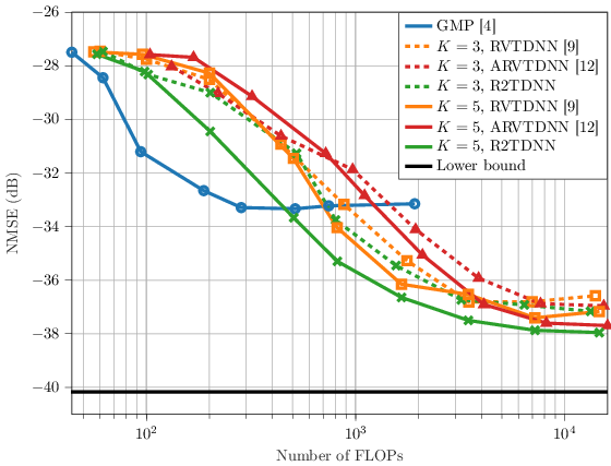
Fig. 4 and Fig. 5 show the normalized mean square error results versus the total number of floating point operations for the generalized memory polynomial [4], real-valued time-delay neural network [9], augmented real-valued time-delay neural network [12], and the proposed residual real-valued time-delay neural network. For the real-valued time-delay neural network and residual real-valued time-delay neural network, we consider two scenarios with one and three hidden layers, i.e., . We also plot the results of the augmented real-valued time-delay neural network [12] for , where we consider three augmented envelop terms of the signal (amplitude and its square and cube) [12, Tab. II] at the input layer. A proper number of memory length is related to the power amplifier characteristics and input signal bandwidth, and here we choose identical input memory for real-valued time-delay neural network, augmented real-valued time-delay neural network, and residual real-valued time-delay neural network. Meanwhile, they use the same number of neurons for each hidden layer. The number of floating point operations increases as the number of neurons for each hidden layer increases. For the generalized memory polynomial (blue circle markers), we select the best results with respect to the number of floating point operations based on an exhaustive search of different values of , , and .
Although the generalized memory polynomial model achieves better normalized mean square error for a number of floating point operations , the performance flattens around dB. The proposed residual real-valued time-delay neural network allows to reach lower normalized mean square error (down to dB) for a number of floating point operations , i.e., the residual real-valued time-delay neural network yields more accurate compensation—it can find a better inverse behavior of the power amplifier. Note that the normalized mean square error gap between the residual real-valued time-delay neural network and the lower bound may be due to the limitation of the indirect learning architecture and some stochastic noise, e.g., phase noise. The adjacent channel power ratio results in Fig. 5 illustrate similar advantages of the residual real-valued time-delay neural network over the generalized memory polynomial for a number of floating point operations .
For comparison, we also plot the performance of the real-valued time-delay neural network in [9] and augmented real-valued time-delay neural network in [12] for . We note that the augmented real-valued time-delay neural network requires a number of floating point operations to improve the performance of real-valued time-delay neural network. However, the proposed residual real-valued time-delay neural network achieves lower normalized mean square error and adjacent channel power ratio with respect to the real-valued time-delay neural network and augmented real-valued time-delay neural network for a similar number of floating point operations. The gain is more considerable for and a number of neurons per hidden layer between and .
IV-B2 Convergence speed comparison
To further compare the real-valued time-delay neural network [9], augmented real-valued time-delay neural network [12], and residual real-valued time-delay neural network, we plot the training and validation errors during the training procedure in Fig. 6. Based on the same parameter setup in Section IV-B1, we select and . The corresponding number of floating point operations, normalized mean square error, and adjacent channel power ratio are given in Table I. Compared to the real-valued time-delay neural network and augmented real-valued time-delay neural network, the residual real-valued time-delay neural network exhibits significantly faster training convergence rate, and eventually achieves lower training and validation errors. This verifies the effectiveness of the proposed residual learning on digital predistortion.
V Conclusion
We applied residual learning to facilitate the learning problem of the power amplifier behavior, and proposed a novel neural network-based power amplifier behavioral model, named residual real-valued time-delay neural network. By adding shortcuts between the input and output layer, the proposed residual real-valued time-delay neural network focus on learning the power amplifier nonlinear behavior instead of learning its whole behavior. We applied different behavioral models to digital predistortion and evaluated the performance on a real power amplifier. Results show that the proposed residual real-valued time-delay neural network achieves lower normalized mean square error and adjacent channel power ratio than the real-valued time-delay neural network and augmented real-valued time-delay neural network previously proposed in the literature with less or similar computational complexity. Furthermore, it has a faster training convergence rate during the training procedure.
References
- [1] N. Kelly, W. Cao, and A. Zhu, “Preparing linearity and efficiency for 5G: Digital predistortion for dual-band Doherty power amplifiers with mixed-mode carrier aggregation,” IEEE Microw. Mag., vol. 18, no. 1, pp. 76–84, Dec. 2016.
- [2] C. Eun and E. J. Powers, “A new Volterra predistorter based on the indirect learning architecture,” IEEE Trans. Signal Process., vol. 45, no. 1, pp. 223–227, Jan. 1997.
- [3] J. Kim and K. Konstantinou, “Digital predistortion of wideband signals based on power amplifier model with memory,” Electron. Lett., vol. 37, no. 23, pp. 1417–1418, Nov. 2001.
- [4] D. R. Morgan, Z. Ma, J. Kim, M. G. Zierdt, and J. Pastalan, “A generalized memory polynomial model for digital predistortion of RF power amplifiers,” IEEE Trans. Signal Process., vol. 54, no. 10, pp. 3852–3860, Oct. 2006.
- [5] J. C. Pedro and S. A. Maas, “A comparative overview of microwave and wireless power-amplifier behavioral modeling approaches,” IEEE Trans. Microw. Theory Tech., vol. 53, no. 4, pp. 1150–1163, Apr. 2005.
- [6] S. Orcioni, “Improving the approximation ability of Volterra series identified with a cross-correlation method,” Nonlinear Dynamics, vol. 78, no. 4, pp. 2861–2869, Dec. 2014.
- [7] M. Isaksson, D. Wisell, and D. Ronnow, “Wide-band dynamic modeling of power amplifiers using radial-basis function neural networks,” IEEE Trans. Microw. Theory Tech., vol. 53, no. 11, pp. 3422–3428, Nov. 2005.
- [8] D. Luongvinh and Y. Kwon, “Behavioral modeling of power amplifiers using fully recurrent neural networks,” in IEEE MTT-S Int. Microw. Symp. Dig., Jun. 2005, pp. 1979–1982.
- [9] T. Liu, S. Boumaiza, and F. M. Ghannouchi, “Dynamic behavioral modeling of 3G power amplifiers using real-valued time-delay neural networks,” IEEE Trans. Microw. Theory Tech., vol. 52, no. 3, pp. 1025–1033, Mar. 2004.
- [10] F. Mkadem and S. Boumaiza, “Physically inspired neural network model for RF power amplifier behavioral modeling and digital predistortion,” IEEE Trans. Microw. Theory Tech., vol. 59, no. 4, pp. 913–923, Jan. 2011.
- [11] T. Gotthans, G. Baudoin, and A. Mbaye, “Digital predistortion with advance/delay neural network and comparison with Volterra derived models,” in IEEE 25th Annual Int. Symp. on Personal, Indoor, and Mobile Radio Commun., Sept. 2014, pp. 811–815.
- [12] D. Wang, M. Aziz, M. Helaoui, and F. M. Ghannouchi, “Augmented real-valued time-delay neural network for compensation of distortions and impairments in wireless transmitters,” IEEE Trans. Neural Netw. Learn. Syst, vol. 30, no. 1, pp. 242–254, Jun. 2018.
- [13] R. Hongyo, Y. Egashira, T. M. Hone, and K. Yamaguchi, “Deep neural network-based digital predistorter for Doherty power amplifiers,” IEEE Microw. Wireless Compon. Lett., vol. 29, no. 2, pp. 146–148, Jan. 2019.
- [14] C. Tarver, A. Balatsoukas-Stimming, and J. R. Cavallaro, “Design and implementation of a neural network based predistorter for enhanced mobile broadband,” arXiv preprint arXiv:1907.00766, 2019.
- [15] J. H. K. Vuolevi, T. Rahkonen, and J. P. A. Manninen, “Measurement technique for characterizing memory effects in RF power amplifiers,” IEEE Trans. Microw. Theory Tech., vol. 49, no. 8, pp. 1383–1389, Aug. 2001.
- [16] A. S. Tehrani, H. Cao, S. Afsardoost, T. Eriksson, M. Isaksson, and C. Fager, “A comparative analysis of the complexity/accuracy tradeoff in power amplifier behavioral models,” IEEE Trans. Microw. Theory Tech., vol. 58, no. 6, pp. 1510–1520, Jun. 2010.
- [17] K. He, X. Zhang, S. Ren, and J. Sun, “Deep residual learning for image recognition,” in IEEE Conf. on Computer Vision and Pattern Recognition (CVPR), Jun. 2016, pp. 770–778.
- [18] P. N. Landin, S. Gustafsson, C. Fager, and T. Eriksson, “Weblab: A web-based setup for PA digital predistortion and characterization [application notes],” IEEE Microw. Mag., vol. 16, no. 1, pp. 138–140, Feb. 2015.
- [19] D. P. Kingma and J. Ba, “Adam: A method for stochastic optimization,” arXiv preprint arXiv:1412.6980, 2014.
- [20] J. Chani-Cahuana, C. Fager, and T. Eriksson, “Lower bound for the normalized mean square error in power amplifier linearization,” IEEE Microw. Wireless Compon. Lett., vol. 28, no. 5, pp. 425–427, May. 2018.