Max-Consensus Over Fading Wireless Channels

Fabio Molinari Navneet Agrawal Sławomir Stańczak and Jörg Raisch Thanks: F. Molinari is with the Control Systems Group - Technische Universität Berlin, Germany. (email: molinari@tu-berlin.de) Thanks: N. Agrawal is with the Network Information Theory Group - Technische Universität Berlin, Germany. (email: navneet.agrawal@tu-berlin.de) Thanks: S. Stańczak is with the Network Information Theory Group - Technische Universität Berlin, Germany & Fraunhofer Heinrich Hertz Institute, Germany. (e-mail: slawomir.stanczak@hhi.fraunhofer.de) Thanks: J. Raisch is with the Control Systems Group - Technische Universität Berlin, Germany (e-mail: raisch@control.tu-berlin.de) Thanks: This work was funded by the German Research Foundation (DFG) within their priority programme SPP1914 "Cyber-Physical Networking",
RA516/12-1 & STA864/10-1

Abstract

The topic of this paper is achieving finite-time max-consensus in a multi-agent system that communicates over a fading wireless channel and exploits its interference property. This phenomenon corrupts the desired information when data is transmitted synchronously. In fact, each transmitted signal is attenuated by an unknown and time-varying factor (fading coefficient), then, by interference, all such attenuated signals are summed up at a receiver. Rather than combatting interference, we design a communication system that exploits it. Our strategy yields a more efficient usage of wireless resources compared to other algorithms. By simultaneously accessing this communication system, each agent obtains a weighted average of the neighbouring agents’ information states. With this piece of information at hand and with a switching consensus protocol employing broadcast authorisations for agents, max-consensus can be achieved within a finite number of iterations.

I Introduction

Consensus is a useful notion in situations where several autonomous intercommunicating agents need to reach an agreement over a variable of common interest, see [28]. Each agent has an estimate of this variable, referred to as information state, which is iteratively updated by running a consensus protocol. This is composed of two subsequent steps: communication and computation. In fact, first, agents share their information states with their neighbors. Subsequently, each agent uses the received pieces of information to update, at every iteration, its information state.

When the system aims at agreeing on the average of initial information states, we talk about average consensus. This has been extensively investigated in literature, see, e.g., [26, 5]. Average consensus is employed in many contexts, e.g., formation control of autonomous vehicles (see [27]), flocking (see [25]), or distributed solution of linear algebraic equations (see [22]). The case of agents seeking for an agreement on the largest information state, namely max-consensus, is also studied in literature, see, e.g., [24]. Its applications range from task allocation (see [4]) to road traffic automation (see [17]), posture control (see [16]), and distributed estimation (see [8]).

Especially in the case when agents are powered by batteries, using resources economically is very important. [31] and [10] introduce a strategy for achieving consensus more efficiently in a wireless communication scenario. This is achieved by exploiting the interference property of the wireless channel, which is traditionally combatted. In fact, in standard wireless settings, interference is a phenomenon that needs to be eliminated. However, as shown in [11], creating an interference-free communication medium for computing functions over the channel is a suboptimal strategy. Therefore, the design of consensus protocols aiming at exploiting interference and, as a consequence, allowing a more efficient use of wireless resources, has recently attracted attention. [20] presents a protocol that achieves average consensus and exploits the interference property of the fading wireless channel. The same is used in [18] for letting agents with single integrator dynamics achieve a desired formation in space. [19] has introduced a consensus-based privacy preserving strategy that exploits interference for distributively solving linear algebraic equations.

To the best of our knowledge, there have been very few attempts to exploit interference for achieving max-consensus. Under the assumption of an ideal channel, [13] proposes a consensus protocol that achieves max-consensus with probability one, by employing a random broadcast strategy. [21] suggests a switching consensus protocol which exploits interference and is proven to achieve max-consensus deterministically. However, these attempts do not deal with the presence of a fading channel, i.e., a channel that attenuates each signal by an unknown factor, which is required for a more realistic analysis. The novelty of this paper is a consensus protocol which (i) achieves max-consensus in a finite number of iterations, (ii) exploits interference, and (iii) can cope with fading channel coefficients.

The paper is structured as follows: in Section II, necessary facts from consensus and communication theory are collected. Section III presents a max-consensus protocol which leads to asymptotic convergence for fading channels. Achieving finite-time max-consensus in the same wireless setting is the topic of Section IV. Randomized simulations show the benefits of this strategy in comparison to standard approaches. Concluding remarks are stated in Section V.

I-A Notation

In the remainder of this paper, $\mathbb{N}_{0}$ denotes the set of nonnegative integers and $\mathbb{N}$ denotes the set of positive integers. The set of real numbers is denoted by $\mathbb{R}$ , while the set of nonnegative, respectively positive, real numbers by $\mathbb{R}_{\geq 0}$ , respectively $\mathbb{R}_{>0}$ . A directed graph is a pair $(\mathcal{N},\mathcal{A})$ , where $\mathcal{N}\subset\mathbb{N}$ is the node set and $\mathcal{A}\subseteq\mathcal{N}\times\mathcal{N}$ the arc set. $(i,j)\in\mathcal{A}$ is an arc from node $i$ to node $j$ . A path from node $i_{1}$ to node $i_{n}$ is a sequence of arcs

(i_{1},i_{2}),(i_{2},i_{3}),\dots,(i_{n-1},i_{n}).

The graph $(\mathcal{N},\mathcal{A})$ is said to be strongly connected if there is a path between all pairs of nodes. Given a finite set $A$ , its cardinality is denoted by $|A|$ . Given a set $A$ , $\mathcal{C}(A)$ denotes the convex hull of $A$ , i.e.

\mathcal{C}(A):=\left\{\sum_{i=1}^{|A|}\lambda_{i}x_{i}\mid{x_{i}}\in A,\lambda_{i}\geq 0,\ \sum_{i=1}^{|A|}\lambda_{i}=1\right\}.

Given a vector $\mathbf{v}\in\mathbb{R}^{n}$ , $n\in\mathbb{N}$ , its element in position $i\in\{1,\dots,n\}$ is $[\mathbf{v}]_{i}$ . The transpose of $\mathbf{v}$ is $\mathbf{v}^{\prime}$ . By $\mathbf{1}_{n}$ , we denote the vector composed of $n$ ones.

Given $x\in\mathbb{R}$ , its absolute value is $|x|$ , $\lceil x\rceil$ denotes the least integer greater than or equal to $x$ , while $\lfloor x\rfloor$ is the greatest integer less than or equal to $x$ .

The indicator function of a set $S\subseteq\mathbb{R}$ , denoted by $I_{S}:\mathbb{R}\mapsto\{0,1\}$ , is defined by $I_{S}(x)=1$ if $x\in S$ and $0$ otherwise.

II System Description

II-A Consensus in Multi-agent Systems

We consider a multi-agent system with $n>1$ agents communicating over the wireless channel and modeled by the directed graph $(\mathcal{N},\mathcal{A})$ . Given an agent $i\in\mathcal{N}$ , $N_{i}\subset\mathcal{N}$ denotes the set of its neighbors, i.e. $N_{i}:=\{j\in\mathcal{N}\mid(j,i)\in\mathcal{A}\}$ .

The multi-agent system seeks for an agreement over a variable of common interest. Each agent $i\in\mathcal{N}$ has an initial estimation of this variable, which is referred to as its initial information state $x_{i_{0}}\in\mathrm{S}:=[S_{\mathrm{min}},S_{\mathrm{max}}]\subset\mathbb{R}_{\geq 0}$ , with $S$ being a compact set. In order to achieve consensus, agents iteratively exchange information with their neighbors and update their information states according to a predefined consensus protocol. Let, $\forall i\in\mathcal{N}$ , $\forall k\in\mathbb{N}_{0}$ , $\mathbf{x}_{N_{i}}(k)\in S^{|N_{i}|}$ be the set of information states of all agents in $N_{i}$ at iteration $k\in\mathbb{N}_{0}$ , i.e.,

\mathbf{x}_{N_{i}}(k):=[x_{j_{1}}(k),\dots,x_{j_{m_{i}}}(k)]^{\prime},

(1)

where $j_{1},\dots,j_{m_{i}}\in N_{i}$ and $m_{i}=|N_{i}|$ . Widely considered discrete-time consensus protocols are of the form

x_{i}(k+1)=f_{i}(x_{i}(k),\mathbf{x}_{N_{i}}(k)),

(2)

where $f_{i}:\mathrm{S}^{|N_{i}|+1}\rightarrow\mathrm{S}$ and, $\forall i\in\mathcal{N}$ , $x_{i}(0)=x_{i_{0}}$ . The information states at iteration $k\in\mathbb{N}_{0}$ are collected in the vector $\mathbf{x}(k)$ , i.e., $\forall i\in\mathcal{N}$ , $[\mathbf{x}(k)]_{i}=x_{i}(k)$ . The system achieves consensus if $\exists x^{*}\in\mathrm{S}$ such that

\forall i\in\mathcal{N},\ \lim\limits_{k\rightarrow\infty}x_{i}(k)=x^{*}.

(3)

The system is said to achieve max-consensus if each information state converges to the largest initial information state of the multi-agent system, i.e.,

\forall i\in\mathcal{N},\ \lim\limits_{k\rightarrow\infty}x_{i}(k)=x^{*}=\max_{i\in\mathcal{N}}({x}_{i_{0}}).

(4)

If an agreement is achieved in a finite number of iterations, then we have finite-time max-consensus. Formally, $\exists\bar{k}\in\mathbb{N}_{0}$ , such that

\forall k>\bar{k},~\forall i\in\mathcal{N},\ x_{i}(k)=x^{*}=\max_{i\in\mathcal{N}}({x}_{i_{0}}).

(5)

Any agent, say $i\in\mathcal{N}$ , whose information state at iteration $k\in\mathbb{N}_{0}$ is $x_{i}(k)=x^{*}=\max_{i\in\mathcal{N}}({x}_{i_{0}})$ is referred to as a maximal agent at iteration $k$ .

II-B Max-Consensus: Benchmarking Protocol

In a standard max-consensus protocol, each agent $i\in\mathcal{N}$ applies, at every iteration $k\in\mathbb{N}_{0}$ , the following update:

x_{i}(k+1)=\max_{j\in N_{i}\cup\{i\}}(x_{j}(k)).

(6)

Therefore, at iteration $k\in\mathbb{N}_{0}$ , each agent $i\in\mathcal{N}$ updates its information state by setting it to the largest value in the set $\{x_{i}(k),x_{j_{1}}(k),\dots,x_{j_{m_{i}}}(k)\}$ . Under the assumption of a time-invariant and connected network topology, [24] shows that max-consensus is achieved in at most $l\in\mathbb{N}$ steps, where

l=\max_{i,j=1,\dots,n}\{|i,j|_{l,\min}\},

(7)

where $|i,j|_{l,\min}$ is the length of the shortest path connecting nodes $i$ and $j$ . Such a consensus protocol can be implemented if each agent has access to its neighbors’ information states. Under a communication point of view, this can be achieved by employing orthogonal channel access methods together with error coding and re-transmission mechanisms (for combatting noise), see [29, Chapter 4]. For benchmarking purposes, we refer to the the joint usage of protocol (6) and orthogonal channel access methods as the standard approach for max-consensus.

In a wireless communication setting, orthogonal access to the communication channel can be ensured, but may cause unacceptable costs in terms of higher overhead. In fact, if the objective is to determine the maximum value in a given set, it is in general not necessary to provide each agent with the complete knowledge of each element in the set. In fact, by the data processing inequality [7], the amount of information contained in the set $\{x_{i}(k),x_{j_{1}}(k),\dots,x_{j_{m_{1}}}(k)\}$ is in general larger than the amount of information carried by $\max_{j\in N_{i}\cup\{i\}}(x_{j}(k))$ . Adopting orthogonal transmission (thus avoiding interference) is therefore not necessary, which motivates a more efficient method to achieve the same goal by exploiting the interference.

II-C Wireless Multiple Access Channel (WMAC)

The WMAC model describes the communication between multiple transmitters and a receiver over the fading wireless channel, see, e.g., [1, 9]. All transmitters access the same channel simultaneously. The fading effect attenuates by a random (and unknown) coefficient all transmitted signals. The receiver obtains a superposition (sum) of such attenuated signals.

Definition 1 (WMAC).

Let $\mathcal{T}\subset\mathcal{N}$ be a subset of agents transmitting to a designated agent $i\in\mathcal{N}$ . Each agent $j\in\mathcal{T}$ at iteration $k\in\mathbb{N}$ transmits a wireless signal $\omega_{j}(k)\in\mathbb{R}$ . The signal obtained by the receiver is $z_{i}(k)\in\mathbb{R}$ , computed as

{z_{i}(k):=\sum_{j\in\mathcal{T}}\xi_{ij}(k)\,\omega_{j}(k),}

(8)

where, $\forall k\in\mathbb{N}_{0}$ , $\forall j\in\mathcal{T}$ , $\xi_{ij}(k)\in\mathbb{R}_{>0}$ is the real fading coefficient that captures the fading effect between the transmitter $j$ and the receiver $i$ .

Under a communication theoretical point of view, the wireless model presented in Definition 1 is based on some assumptions.

Assumption 1 (Wireless Channel).

(A1)

The fading channel coefficients are assumed to be positive real numbers. This is possible by employing a communication system as in [12], [14], and [3].
(A2)

The fading channel coefficients are assumed to be identically distributed and independent across different iterations and across different transmitter-receiver pairs. This is a valid assumption when the channel is fast-fading, see, e.g., [29, Ch 2.3]. As in [29, Ch 2.4], channel coefficients are drawn out of a Rayleigh or Rician distribution¹¹ 1 The Rayleigh distribution is widely used to model non-line-of-sight scenarios, while the Rician distribution is assumed if a strong line-of-sight component is present. .
(A3)

The receiver is assumed to have no additive noise. Indeed, in a high-SNR (Signal to Noise Ratio) regime, receiver noise can be neglected.
(A4)

Transmission and reception of wireless signals take place simultaneously across the network at every iteration $k\in\mathbb{N}$ . This is possible by employing full-duplex transceivers, see, e.g., [6].

II-D Communication System

The goal of our communication system is to provide each agent $i\in\mathcal{N}$ at every iteration $k\in\mathbb{N}_{0}$ with a signal $u_{i}(k)$ such that

u_{i}(k)\in\mathcal{C}\left(\{x_{j}(k)\}_{j\in N_{i}}\right),

(9)

where $\mathcal{C}$ denotes the convex-hull and $N_{i}$ is the set that includes all agents transmitting to agent $i$ (namely, its neighbors)²² 2 We assume $N_{i}$ to be non-empty. . This is possible by designing a communication system that processes the signal both at each transmitter and at the receiver.

II-D1 Transmitter-side processing

All transmitters have the same power constraints which restrict the amplitude of transmitted signals to a finite range, i.e., $\mathrm{P}:=[P_{\min},P_{\max}]\subset\mathbb{R}_{\geq 0}$ . Before transmission, the information state $x_{j}$ of an agent $j$ is transformed using an affine function $\Phi:\mathrm{S}\to\mathrm{P}$ such that

\Phi(x)=\alpha x+\beta,

(10)

where

\alpha=\frac{P_{\max}-P_{\min}}{S_{\max}-S_{\min}}\in\mathbb{R}_{>0}

and

\beta=P_{\min}-\alpha S_{\min}.

The signal transmitted by agent $j$ at iteration $k$ is

\mu_{j}(k)=\Phi(x_{j}(k)).

Also, as it will become clear in the receiver-side processing section, in order for the receiver to normalize the fading coefficients, a dummy signal $\mu^{\prime}_{j}(k)$ is transmitted (orthogonal to $\mu_{j}(k)$ ). Signal $\mu^{\prime}_{j}(k)$ is given by, $\forall j\in N_{i}$ , $\forall k\in\mathbb{N}_{0}$ ,

\mu^{\prime}_{j}(k)=\Phi(1)=\alpha+\beta.

II-D2 Receiver-side processing

By the WMAC model (see Definition 1), each receiver $i\in\mathcal{N}$ obtains two real-valued orthogonal signals at every iteration $k\in\mathbb{N}$ , which are

	$\displaystyle r_{i}(k)$	$\displaystyle:=\sum_{j\in N_{i}}\xi_{ij}(k)\mu_{j}(k)=\sum_{j\in N_{i}}\xi_{ij}(k)(\alpha x_{j}(k)+\beta),$		(11)
	$\displaystyle r^{\prime}_{i}(k)$	$\displaystyle:=\sum_{j\in N_{i}}\xi_{ij}(k)\mu^{\prime}_{j}(k)=(\alpha+\beta)\sum_{j\in N_{i}}\xi_{ij}(k).$		(11)

At the receiver, we apply a de-scaling transformation $\Psi:\mathbb{R}^{2}\to\mathbb{R}$ that is

\Psi(r_{i},r^{\prime}_{i}):=\frac{1}{\alpha}(r_{i}-\frac{\beta}{\alpha+\beta}r^{\prime}_{i})=\sum_{j\in N_{i}}\xi_{ij}(k)x_{j}(k),

(12)

where $\alpha$ and $\beta$ are the values introduced in (10). With this information at hand, each agent $i\in\mathcal{N}$ can obtain signal (9) at every iteration $k\in\mathbb{N}_{0}$ by computing

u_{i}(k)=\cfrac{(\alpha+\beta)\Psi(r_{i},r^{\prime}_{i})}{r^{\prime}_{i}}.

(13)

By inserting (12) and (11) into (13), one obtains

u_{i}(k)=\sum_{j\in N_{i}}h_{ij}(k)x_{j}(k),

(14)

where, $\forall i,j\in\mathcal{N}$ , $\forall k\in\mathbb{N}_{0}$ , $h_{ij}(k)\in\mathbb{R}>0$ is referred to as the normalized channel coefficient corresponding to the transmission from $j$ to $i$ at iteration $k$ and can be formally expressed as

h_{ij}(k):=\frac{\xi_{ij}(k)}{\sum_{q\in N_{i}}\xi_{iq}(k)}\ \in(0,1].

(15)

Note that each normalized channel coefficient is unknown. However, they sum up to $1$ , i.e., $\forall i\in\mathcal{N}$ , $\forall k\in\mathbb{N}_{0}$ ,

\sum_{j\in N_{i}}h_{ij}(k)=1.

This proves that the requirement (9) is satisfied.

III Asymptotic Max-Consensus Protocol

III-A Max-Consensus Protocol Design

In the following, we describe a max-consensus protocol for the multi-agent system from Section II-A and the communication system from Section II-D. It exploits interference and is based on two underlying ideas, which are summarized in Observation 1 and Proposition 1.

Observation 1.

If the goal is to achieve max-consensus, any non-maximal agent at iteration $k\in\mathbb{N}_{0}$ does not need to communicate its own information state at iteration $k\in\mathbb{N}_{0}$ .

However, agents in general do not know whether they are maximal at a given iteration $k$ . Agents only have a local estimation of this. Let us assume that the result of this local evaluation for agent $i\in\mathcal{N}$ at iteration $k\in\mathbb{N}_{0}$ is stored in a binary variable $\tilde{y}_{i}(k)\in\{0,1\}$ . In the case $\tilde{y}_{i}(k)=1$ , agent $i\in\mathcal{N}$ is said to be a maximal-candidate at iteration $k$ . If (and only if) agent $i$ is a maximal-candidate, it will be allowed to broadcast at the next iteration. This will be expressed by an authorization variable $y_{i}:\mathbb{N}_{0}\rightarrow\{0,1\}$ , where $y_{i}(k)=\tilde{y}_{i}(k-1)$ and $y_{i}(0)=1$ .

Now, let,

\forall i\in\mathcal{N},~\forall k\in\mathbb{N}_{0},\\ N_{i}^{m}(k):=\{j\in N_{i}\mid y_{j}(k)=1\}\subseteq{N}_{i}

(16)

be the set of neighbors authorized to broadcast at iteration $k$ . If only authorized agents broadcast and the communication system of Section II-D is employed, each agent $i\in\mathcal{N}$ will receive, at $k\in\mathbb{N}_{0}$ ,

u_{i}(k)={\sum\limits_{j\in N_{i}^{m}(k)}h_{ij}(k)x_{j}(k)}.

(17)

The local evaluation that establishes which agents are authorized to broadcast is based on the following proposition.

Proposition 1.

Given a set of agents $\mathcal{N}$ , a non-empty subset $\mathcal{M}\subseteq\mathcal{N}$ , and a set of real-valued parameters $\mathcal{H}=\{h_{j}\in(0,1]\mid j\in\mathcal{M}\}$ with $\sum_{j\in\mathcal{M}}h_{j}=1$ , the following holds $\forall k\in\mathbb{N}_{0}$ , $\forall i\in\mathcal{N}$ ,

x_{i}(k)<{\sum_{j\in\mathcal{M}}h_{j}x_{j}(k)}\implies x_{i}(k)<\max_{j\in\mathcal{N}}(x_{j}(k)).

(18)

Proof.

By definition of a convex hull, ${\sum_{j\in\mathcal{M}}h_{j}x_{j}(k)}\in\mathcal{C}(\{x_{j}(k)\mid j\in\mathcal{M}\}).$ Moreover, $\forall p\in\mathcal{C}(\{x_{j}(k)\mid j\in\mathcal{M}\}):\ p\leq\max_{j\in\mathcal{M}}(x_{j}(k))$ . Hence,

{\sum_{j\in\mathcal{M}}h_{j}x_{j}(k)}\leq\max_{j\in\mathcal{M}}(x_{j}(k)).

Since $\mathcal{M}\subseteq\mathcal{N}$ ,

x_{i}(k)<\max_{j\in\mathcal{M}}(x_{j}(k))\leq\max_{j\in\mathcal{N}}(x_{j}(k)).

This implies (18). ∎

By (18), for $\mathcal{M}=N_{i}^{m}(k)$ and $\mathcal{H}=\{h_{ij}(k)\mid j\in N_{i}^{m}(k)\}$ , the implication

x_{i}(k)<u_{i}(k)\implies x_{i}(k)<\max_{j\in\mathcal{N}}({x}_{j}(k))

(19)

immediately follows. Therefore, $y_{i}$ can be updated as

\forall i\in\mathcal{N},~\forall k\in\mathbb{N}_{0},\\ y_{i}(k+1)=\tilde{y}(k)=I_{\mathbb{R}\geq 0}(x_{i}(k)-u_{i}(k)).

(20)

In the light of these observations, and given that the signal $u_{i}(k)$ is computed by harnessing the interference of the channel, each agent $i\in\mathcal{N}$ can apply the following max-consensus protocol:

\forall k\in\mathbb{N}_{0},\ \begin{cases}x_{i}(k+1)=\max(x_{i}(k),u_{i}(k))\\ y_{i}(k+1)=I_{\mathbb{R}_{\geq 0}}(x_{i}(k)-u_{i}(k))\end{cases},

(21)

where $y_{i}(0)=1$ and $x_{i}(0)=x_{i_{0}}\in\mathrm{S}$ , and $u_{i}(k)$ is obtained from (17). Note that $u_{i}(k)$ is determined by $x_{j}(k)$ and $y_{j}(k)$ , $j\in N_{i}$ . (17)-(21) can then be rewritten in vector-form as

\mathbf{w}(k+1)=g(\mathbf{w}(k)),

(22)

where

\mathbf{w}(k)=\left[\begin{matrix}\mathbf{x}(k)\\ \mathbf{y}(k)\end{matrix}\right],

(23)

and, $\forall i\in\mathcal{N},~[\mathbf{x}(k)]_{i}=x_{i}(k),~[\mathbf{y}(k)]_{i}=y_{i}(k)$ , and $g:\mathbb{R}^{n}\times\{0,1\}^{n}\rightarrow\mathbb{R}^{n}\times\{0,1\}^{n}$ is the nonlinear function reflecting (21) and (17).

III-B Asymptotic Convergence of the System

A multi-agent system with a strongly connected network topology $(\mathcal{N},\mathcal{A})$ is given. The system uses the consensus protocol (22), i.e., each agent iterates (17),(21) synchronously. In the following, we prove asymptotic convergence by using Lyapunov theory (cf. [2, p. 87] and [15, p. 22]). Initially, we show that all information states are non-decreasing bounded sequences.

Proposition 2.

Given a multi-agent system with network topology $(\mathcal{N},\mathcal{A})$ and consensus protocol (22), $\forall\mathbf{x}(0)\in\mathrm{S}^{n}$ , $\forall i\in\mathcal{N}$ , $\forall k\in\mathbb{N}_{0}$ ,

x_{i}(k)\leq x_{i}(k+1)\leq\max_{j\in\mathcal{N}}({x}_{j}(0)).

(24)

Proof.

The first inequality immediately follows from (21). The second inequality follows from the fact that, according to (17),

u_{i}(k)\in\mathcal{C}\left(\{x_{j}(k)\mid N_{i}^{m}(k)\}\right)

if $N_{i}^{m}(k)\not=\emptyset$ , zero else. Hence

u_{i}(k)\leq\max_{j\in N_{i}^{m}(k)}\left(x_{j}(k)\right)\leq\max_{j\in\mathcal{N}}\left(x_{j}(k)\right).

Therefore, $\forall i\in\mathcal{N}$ ,

x_{i}(k+1)\leq\max_{j\in N_{i}^{m}(k)}\left(x_{j}(k)\right)\leq\max_{j\in\mathcal{N}}\left(x_{j}(k)\right).

Moreover,

\max_{j\in\mathcal{N}}\left(x_{j}(k+1)\right)\leq\max_{j\in\mathcal{N}}\left(x_{j}(k)\right),

thus yielding the second inequality. ∎

The following propositions establish a unique equilibrium point.

Proposition 3.

\mathbf{w}^{*}=\left[{\mathbf{x}^{*}}^{\prime},\mathbf{1}_{n}^{\prime}\right]^{\prime},

(25)

with $\mathbf{x}^{*}=x^{*}\mathbf{1}_{n}$ and $x^{*}=\max_{j\in\mathcal{N}}({x}_{j}(0))$ is an equilibrium point for the multi-agent system with network topology $(\mathcal{N},\mathcal{A})$ and consensus protocol (22).

Proof.

Assume $\mathbf{w}(k)=\mathbf{w}^{*}$ . This implies, $\forall i\in\mathcal{N}$ , $x_{i}(k)=x^{*}$ and $y_{i}(k)=1$ . Therefore $N_{i}^{m}(k)=N_{i}$ , hence

	$\displaystyle u_{i}(k)$	$\displaystyle=\sum_{j\in N_{i}}h_{ij}(k)x_{j}(k)$
		$\displaystyle=\left(\sum_{j\in N_{i}}h_{ij}(k)\right)x^{}=x^{},$		(26)

as $N_{i}\not=\emptyset$ . Then, according to (21),

	$\displaystyle x_{i}(k+1)$	$\displaystyle=\max(x^{},u_{i}(k))=x^{}$	(27)
and
	$\displaystyle y_{i}(k+1)$	$\displaystyle=I_{\mathbb{R}_{\geq 0}}\left(x^{*}-u_{i}(k)\right)=1,$	(28)

and, therefore, $\mathbf{w}(k+1)=\mathbf{w}^{*}$ . ∎

Proposition 4.

Consider a multi-agent system with a strongly connected network topology $(\mathcal{N},\mathcal{A})$ using the consensus protocol (21).

\mathbf{w}^{*}=\left[{x}^{*}\mathbf{1}_{n}^{\prime},\mathbf{1}_{n}^{\prime}\right]^{\prime}

is the unique equilibrium point.

Proof.

The proof is by contradiction, i.e., we assume that there exists an equilibrium point

\hat{\mathbf{w}}=[\hat{\mathbf{x}}^{\prime},\hat{\mathbf{y}}^{\prime}]^{\prime}\not=\mathbf{w}^{*}.

Case 1

$\hat{\mathbf{y}}\not=\mathbf{1}_{n}^{\prime}$ , i.e.,

\exists i\in\mathcal{N},~\text{s.t.}~\hat{\mathbf{y}}_{i}=0.

Hence, because of (21),

x_{i}(k)<u_{i}(k)

and therefore $x_{i}(k+1)>x_{i}(k)$ . Hence we have established that for any equilibrium point $\hat{\mathbf{w}}$ the Boolean part needs to be

\hat{\mathbf{y}}=\mathbf{1}_{n}^{\prime}.

Case 2

$\hat{\mathbf{y}}=\mathbf{1}_{n}^{\prime}.$ but $\hat{\mathbf{x}}\not=x^{*}\mathbf{1}_{n}^{\prime}$ . Because of the first premise, $\forall i\in\mathcal{N}$ ,

N_{i}^{m}(k)=N_{i}.

As $(\mathcal{N},\mathcal{A})$ is strongly connected, $N_{i}\not=\emptyset$ , $\forall i\in\mathcal{N}$ . Furthermore, also because of $(\mathcal{N},\mathcal{A})$ being strongly connected, there exists a minimal element $l\in\mathcal{N}$ that has at least one non-minimal neighbor, i.e.,

\hat{x}_{l}=\min_{j\in\mathcal{N}}\hat{x}_{j}

and

\hat{x}_{l}<\max_{j\in N_{l}}\hat{x}_{j}:=\hat{x}_{p}.

As the channel coefficients are positive, (17) implies

u_{l}(k)>x_{l}(k).

This and (21) imply

x_{l}(k+1)>x_{l}(k).

Hence, we have established that for any equilibrium point $\hat{\mathbf{w}}$ , the real part has to be $x^{*}\mathbf{1}_{n}$ . ∎

Lemma 1.

Consider a multi-agent system with a strongly connected network topology $(\mathcal{N},\mathcal{A})$ . If protocol (22) is employed, then, $\forall\mathbf{x}(0)\in\mathrm{S}^{n}$ , $\forall k\in\mathbb{N}_{0}$ ,

\sum_{i\in\mathcal{N}}\left(x_{i}(k+2)-x_{i}(k)\right)=0\implies\mathbf{x}(k)=\mathbf{x}^{*}.

(29)

Proof.

From Proposition 2, $\{x_{i}(k)\}_{k\in\mathbb{N}_{0}}$ is a non-decreasing bounded sequence, composed of nonnegative entries. As a consequence, $\sum_{i\in\mathcal{N}}\left(x_{i}(k+2)-x_{i}(k)\right)=0$ if and only if

\mathbf{x}(k)=\mathbf{x}(k+1)=\mathbf{x}(k+2).

(30)

The latter, by (21), implies that, $\forall i\in\mathcal{N},\ x_{i}(k)\geq u_{i}(k)$ and $x_{i}(k+1)\geq u_{i}(k+1)$ . By (20), this implies that

\mathbf{y}(k+1)=\mathbf{y}(k+2)=1.

(31)

From (30) and (31), it clearly follows that

\mathbf{w}(k+1)=\begin{bmatrix}\mathbf{x}(k+1)\\ \mathbf{y}(k+1)\end{bmatrix}=\begin{bmatrix}\mathbf{x}(k+2)\\ \mathbf{y}(k+2)\end{bmatrix}=\mathbf{w}(k+2)

(32)

is an equilibrium for the system. According to Proposition 4, it is unique, i.e.,

\mathbf{w}(k+1)=\mathbf{w}(k+2)=\mathbf{w}^{*},

(33)

\mathbf{x}(k+1)=\mathbf{x}(k+2)=\mathbf{x}^{*}.

(34)

By (30), $\mathbf{x}(k)=\mathbf{x}^{*}$ ; this concludes the proof. ∎

Corollary 1.

Consider a multi-agent system with a strongly connected network topology $(\mathcal{N},\mathcal{A})$ . If the protocol (22) is employed, then, $\forall\mathbf{x}(0)\in\mathrm{S}^{n}$ , $\forall k\in\mathbb{N}_{0}$ ,

\mathbf{x}(k)\not=\mathbf{x}^{*}\implies\sum_{i\in\mathcal{N}}\left(x_{i}(k+2)-x_{i}(k)\right)>0.

(35)

Proof.

(29) is equivalent to

\mathbf{x}(k)\not=\mathbf{x}^{*}\implies\sum_{i\in\mathcal{N}}(x_{i}(k+2)-x_{i}(k))\not=0.

Non-decreasingness of the sequence $\{x_{i}(k)\}_{k\in\mathbb{N}_{0}}$ (Proposition 2) then establishes (35). ∎

By [30, p. 264] and [23, p. 43], a Lyapunov-based analysis can be applied to the discrete-time system like (22), as existence and uniqueness of an equilibrium point have been established in Proposition 3 and Proposition 4.

Theorem 1.

Consider a multi-agent system with a strongly connected network topology $(\mathcal{N},\mathcal{A})$ . Agents employ the consensus protocol (22). For every possible initial state $\mathbf{x}(0)\in\mathrm{S}^{n}$ , the system achieves max-consensus asymptotically.

Proof.

The component $y_{i}$ of (21) can be explicitly rewritten, $\forall k\in\mathbb{N}_{0}$ , as

\displaystyle y_{i}(k+1)=\begin{cases}1&\text{if }x_{i}(k)\geq u_{i}(k)\\ 0&\text{if }x_{i}(k)<u_{i}(k)\end{cases}.

(36)

By (21) and since $\{x_{i}(k)\}_{k\in\mathbb{N}_{0}}$ is a non-decreasing sequence, (36) can be reformulated, $\forall k\in\mathbb{N}_{0}$ , as

\displaystyle y_{i}(k+1)=\begin{cases}1&\text{if }x_{i}(k)=x_{i}(k+1)\\ 0&\text{if }x_{i}(k)<x_{i}(k+1)\end{cases}.

(37)

This, again because of non-decreasingness of $\{x_{i}(k)\}_{k\in\mathbb{N}_{0}}$ , is equivalent to

\displaystyle\forall k\in\mathbb{N}_{0},\ y_{i}(k+1)=I_{\mathbb{R}_{\geq 0}}(x_{i}(k)-x_{i}(k+1)).

(38)

By introducing the new state vector

\mathbf{v}(k):=\left[\begin{matrix}\mathbf{v}_{1}(k)\\ \mathbf{v}_{2}(k)\end{matrix}\right]:=\left[\begin{matrix}\mathbf{x}(k)\\ \mathbf{x}(k-1)\end{matrix}\right].

(39)

we can rewrite (22) as

\mathbf{v}(k+1)=\tilde{g}(\mathbf{v}(k)),

(40)

where the function $\tilde{g}:S^{2n}\mapsto S^{2n}$ can be explicitly expressed by

	$\displaystyle\mathbf{v}_{1}(k+1)$	$\displaystyle=\max(\mathbf{v}_{1}(k),H(k)\mathbf{v}_{1}(k))$		(41)
	$\displaystyle\mathbf{v}_{2}(k+1)$	$\displaystyle=\mathbf{v}_{1}(k),$		(42)

where $\max(\cdot)$ is understood element-wise and

[H(k)]_{ij}:=\begin{cases}h_{ij}(k)\qquad\text{if }j\in N_{i}~\text{and}~[\mathbf{v}_{1}(k)]_{j}=[\mathbf{v}_{2}(k)]_{j}\\ 0\qquad\qquad\text{else}\end{cases}.

Consequently, the unique equilibrium $\mathbf{w}^{*}$ of (22) corresponds to the following unique equilibrium $\mathbf{v}^{*}$ of (40):

\mathbf{v}^{*}=x^{*}\mathbf{1}_{2n}.

(43)

A candidate Lyapunov function $V:\mathrm{S}^{2n}\rightarrow\mathbb{R}_{\geq 0}$ is chosen as follows:

	$\displaystyle\forall k\in\mathbb{N}_{0},\ V(\mathbf{v}(k))$	$\displaystyle=\mathbf{1}_{2n}(\mathbf{v}^{*}-\mathbf{v}(k))$		(44)
		$\displaystyle=2nx^{*}-\sum_{i\in\mathcal{N}}(x_{i}(k)+x_{i}(k-1)).$		(45)

The following properties hold:

a)

$V(\mathbf{v})$ is continuous in $\mathbb{R}_{\geq 0}^{2n}$ ;
b)

$V(\mathbf{v}^{*})=0$ ;
c)

$V(\mathbf{v})$ is positive on any trajectory $\mathbf{v}$ of the system, unless $\mathbf{v}=\mathbf{v}^{*}$ .

This follow directly from Proposition 2.

By Corollary 1, $\forall\mathbf{v}(k)\not=\mathbf{v}^{*}$ (i.e., $\forall\mathbf{x}(k-1)\not=\mathbf{x}^{*}$ ),

	$\displaystyle\Delta V(\mathbf{v}(k))$	$\displaystyle=V(\mathbf{v}(k+1))-V(\mathbf{v}(k))$
		$\displaystyle=-\sum_{i\in\mathcal{N}}\left(x_{i}(k+1)-x_{i}(k-1)\right)<0.$

Hence, the function $V(\mathbf{v})$ has all the properties required for a Lyapunov function. By [15, p. 22] and [2, p. 88], the system therefore asymptotically converges to max-consensus. ∎

In the following corollary, an immediate result coming as a consequence from Theorem 1 is reviewed. It will be used in the next section.

(a) Network topology for Examples 1, 2, 4. The node set is

\{a,b,c,d\}

and the vector of initial information states is

\mathbf{x}(0)=[3,4,3,3]^{\prime}

for Example 1 and 4, and

\mathbf{x}(0)=[3.1,4,3,3]^{\prime}

for Example 2.

(b) Network topology for Example 3. The node set is

\{a,b,c,d\}

and the vector of initial information states is

\mathbf{x}(0)=[3,4,3,3]^{\prime}

Fig. 1: Network topologies considered in Examples 1-4.

Fig. 2: Evolution of agents’ information states for Example 1. The dashed lines represent

x_{a}(k)

and

x_{d}(k)

(which coincide). The red solid line represents the information state of agent

c

. Asymptotic convergence to the max value, i.e.,

x^{*}=x_{b}(0)

, can be observed.

Fig. 3: Evolution of agents’ information states for Example 2. The dashed lines represent the information states of agents

a

and

d

, the solid line that of agent

c

. Max-consensus

x_{b}(0)

is achieved after

4

iterations.

Corollary 2.

Consider a multi-agent system with a strongly connected network topology $(\mathcal{N},\mathcal{A})$ iterating consensus protocol (22).

{\color[rgb]{0,0,0}{\forall i\in\mathcal{N},~x_{i}(k_{0})<x^{*}\implies\exists k_{i}>k_{0}:\ y_{i}(k_{i})=0.}}

(46)

Proof.

Let $\ x^{*}-x_{i}(k_{0})=\epsilon_{0}$ . Choose $\epsilon<\epsilon_{0}$ . Asymptotic stability implies that $\exists k_{\epsilon}>k_{0}$ such that $x^{*}-x_{i}(k)<\epsilon$ , $\forall k>k_{\epsilon}$ . Hence, $x_{i}(k)>x_{i}(k_{0})$ , $\forall k>k_{\epsilon}$ . This implies that $\exists k_{i}$ , $k_{0}<k_{i}\leq k_{\epsilon}$ s.t.

x_{i}(k_{i})-x_{i}(k_{i}-1)>0,

therefore $y_{i}(k_{i})=0$ . ∎

The interpretation of this corollary is that an agent which is non-maximal at iteration $k_{0}$ , will eventually lose its status as a maximal candidate and therefore its authorization to broadcast.

In conclusion, we have shown that a multi-agent system with a strongly connected network topology achieves max-consensus asymptotically by employing protocol (22). This protocol harnesses the interference property of the channel for computing the signal $u_{i}$ . In the following, we show simulation studies that provide further information on convergence and computational benefits of the suggested approach.

III-C Simulations

In the following, some simulation results are presented. The aim is to compare our approach to standard approaches and quantify benefits (saved wireless resources). However, as it will be clear in the simulations, there are cases in which finite-time convergence cannot be achieved with protocol (22), but only asymptotic convergence. In such cases, we cannot quantify benefits. This will motivate the search for an extended protocol in the next section.
Example 1: first, we review a numerical experiment in [21], where channel coefficients are equal and constant. Consider the underlying network in Figure 1(a)-1(b). By (17), $u_{i}(k)$ is the linear average of information states of agents in $N_{i}^{m}(k)$ . Example 1 illustrates asymptotic convergence of a system composed of 4 nodes, with a strongly connected network topology, endowed with protocol (22), see Figure 2.
Examples 2-3: on the other hand, Examples 2, respectively Example 3, show that, by slightly varying $\mathbf{x}(0)$ , respectively the network topology, the system achieves finite-time max-consensus (see Figures 3 and 4). This behavior has been confirmed by running extensive numerical simulations: in most cases, finite time convergence, rather than asymptotic convergence, is achieved.
Examples 4: (see Figure 5), channel coefficients are randomly drawn out of a Rayleigh distribution with variance 1 independently for every iteration. Numerical experiments indicate that the system is very likely to achieve finite-time max-consensus. However, it will be possible to choose a collection of constant channel coefficients, i.e. $\forall k\in\mathbb{N}_{0},\ h_{ji}(k)=h$ , so that consensus is achieved asymptotically, rather than finite-time.
These examples illustrate that the use of protocol (21) for a strongly connected network does not guarantee finite-time consensus. Asymptotic convergence is guaranteed by Theorem 1; the achievement of finite-time consensus, on the other hand, depends on the network topology, the initial information states, and the channel coefficients if protocol (21) is used. This is the motivation for establishing an extended max-consensus protocol in the next section.

Fig. 4: Evolution of agents’ information states for Example 3. The dashed lines represent the information states of agents

a

and

d

, the solid line that of agent

c

. Max-consensus

x_{b}(0)

is achieved after

7

iterations.

Fig. 5: Evolution of agents’ information states in the case of a fading wireless channel. This has an important impact on the convergence: with regards to Figure 2 (nonfading channel), convergence is here achieved in a finite number of steps, rather than asymptotically.

IV Finite-time Max-Consensus Protocol

In this section, an extended max-consensus protocol is presented. It also exploits the channel superposition property. However, in contrast to the protocol (22), it guarantees finite-time convergence for strongly connected network topologies.

IV-A Key idea

Let, $\forall k\in\mathbb{N}_{0}$ , $\mathcal{M}_{k}$ be the set of maximal-agents at iteration $k$ , i.e. $\mathcal{M}_{k}=\{i\in\mathcal{N}\mid x_{i}(k)=x^{*}\}$ . The following proposition states that, at any iteration, there exists a non-maximal agent if and only if there is a non-maximal agent in whose neighborhood there is a maximal agent.

Proposition 5.

Given a multi-agent system with a strongly connected network topology $(\mathcal{N},\mathcal{A})$ , then

\exists j\in\mathcal{N}\setminus\mathcal{M}_{k}\iff\exists i\in\mathcal{N}\setminus\mathcal{M}_{k}~\mathrm{such~that}~N_{i}\cap\mathcal{M}_{k}\not=\emptyset

Proof.

$\impliedby$

Trivial.
$\implies$

Partition $\mathcal{N}$ as $\mathcal{M}_{k}$ and $\mathcal{N}\setminus\mathcal{M}_{k}$ . Choose $j\in\mathcal{N}\setminus\mathcal{M}_{k}$ and $\bar{j}\in\mathcal{M}_{k}$ . Because of strong connectedness, there is a path from $\bar{j}$ to $j$ . Clearly, there is at least one arc in this path, say $(\bar{i},i)$ , such that $\bar{i}\in\mathcal{M}_{k}$ and $i\in\mathcal{N}\setminus\mathcal{M}_{k}$ . As $\bar{i}$ is a neighbour of $i$ , then $\bar{i}\in N_{i}\cap\mathcal{M}_{k}$ .

∎

The following result is derived directly from Corollary 2.

Proposition 6.

Given a multi-agent system with a strongly connected network topology $(\mathcal{N},\mathcal{A})$ endowed with the consensus protocol (22), given an arbitrary $k_{0}\in\mathbb{N}_{0}$ and $\forall\mathbf{x}(k_{0})\in\mathrm{S}^{n}$ , the following holds:

\exists\tilde{k}>k_{0}:\ \forall i\in\mathcal{N}\setminus\mathcal{M}_{k_{0}},\ \prod_{t=k_{0}}^{\tilde{k}}y_{i}(t)=0.

(47)

Proof.

Corollary 2 states that for each $i\in\mathcal{N}\setminus\mathcal{M}_{k_{0}}$ , there exists $k_{i}>k_{0}$ such that $y_{i}(k_{i})=0$ . Take

\tilde{k}:=\max_{i\in\mathcal{N}\setminus\mathcal{M}_{k_{0}}}k_{i}.

Then, $\forall i\in\mathcal{N}\setminus\mathcal{M}_{k_{0}}$ ,

\prod_{t=k_{0}}^{\tilde{k}}y_{i}(t)=0.

The proof is concluded. ∎

By Proposition 6, each agent of the system, say agent $i$ , that at $k_{0}$ is not maximal (i.e. $x_{i}(k_{0})<x^{*}$ ), within $(\tilde{k}-k_{0})$ steps will receive an input $u_{i}(k)$ , $k\in[k_{0},\tilde{k}-1]$ , such that $u_{i}(k)>x_{i}(k)$ .
Now suppose that we change the consensus protocol (21) by setting the authorization variable of each agent $i\in\mathcal{N}$ at iteration $\tilde{k}+1$ to

y_{i}(\tilde{k}+1)=\prod_{t=k_{0}}^{\tilde{k}}y_{i}(t).

(48)

From Proposition 6, this quantity is zero for all agents that were non-maximal at $k_{0}$ , implying that

\forall i\in\mathcal{N},\ N_{i}\cap\mathcal{M}_{k_{0}}\not=\emptyset\implies x_{i}(\tilde{k}+2)=x^{*}.

(49)

In other words, all agents in the neighborhood of a maximal agent will become maximal at iteration $\tilde{k}+2$ .

However, since agents do not have the global knowledge of the system, the value of $\tilde{k}$ is not known a priori. Hence, there will be the need for each agent $i\in\mathcal{N}$ to retain a state variable, say $T_{i}:\mathbb{N}_{0}\rightarrow\mathbb{N}$ , that attempts to (over-)estimate $\tilde{k}$ . By letting $T_{i}(k)$ grow according to a nondecreasing diverging sequence, it will be eventually large enough to over-approximate $\tilde{k}$ .

IV-B Protocol Design

The idea just presented inspires the following switching consensus protocol $\forall i\in\mathcal{N}$ , $\forall k\in\mathbb{N}_{0}$ ,


if $k=2T_{i}(k)$ :
	$\displaystyle\begin{cases}x_{i}(k+1)=\max(x_{i}(k),u_{i}(k))\\ y_{i}(k+1)=\prod_{t=T_{i}(k)}^{k}y_{i}(t)\\ T_{i}(k+1)=k\end{cases},$	(50b)
else:
	$\displaystyle\begin{cases}x_{i}(k+1)=\max(x_{i}(k),u_{i}(k))\\ y_{i}(k+1)=I_{\mathbb{R}_{\geq 0}}(x_{i}(k)-u_{i}(k))\\ T_{i}(k+1)=T_{i}(k)\end{cases},$	(50c)

where $\forall i\in\mathcal{N}$ , $y_{i}(0)=1$ , $x_{i}(0)=x_{i_{0}}$ , $T_{i}(0)=T(0)=2$ , and $\forall i\in\mathcal{N}$ , $\forall k\in\mathbb{N}_{0}$ , $u_{i}(k)$ is computed as in (17), by exploiting the superposition property of the channel. Protocol (50c) is identical to protocol (21), except for the trivial presence of $T_{i}(k)$ , which is, however, kept constant and does not affect the system behavior. Only for iteration steps $k=2^{n},\ n\in\mathbb{N}$ , the proposed consensus protocol switches to (50b).

Proposition 7.

$\forall i\in\mathcal{N}$ , $\forall k\in\mathbb{N}_{0}$ ,

T_{i}(k)=2^{p(k)}\ ,

(51)

where

p(k):=\begin{cases}\lceil\log_{2}(k)-1\rceil&\text{if }k\geq 2\\ 1&\text{else}\end{cases}.

(52)

Proof.

Follows directly from (50). ∎

Proposition 7 implies that $T_{i}(k)$ , $k\in\mathbb{N}_{0}$ , is a non-decreasing diverging sequence.

Remark 1.

The state variable $T_{i}(k)$ is the same for all $i\in\mathcal{N}$ , therefore, the index $i$ can be omitted.

Corollary 3.

A multi-agent system with a strongly connected network topology $(\mathcal{N},\mathcal{A})$ employs switching consensus protocol (50). Then, $\forall\mathbf{x}(0)\in\mathrm{S}^{n}$ ,

\exists k_{s}\in\mathbb{N}_{0}:\ \forall k\geq k_{s},\ T(k)\geq\tilde{k}.

(53)

Proof.

By construction, $T(k)$ is a non-decreasing unbounded sequence. ∎

Remark 2.

It is straightforward to come up with a suitable $k_{s}$ . In fact,

T(k)\geq\tilde{k}\iff\lceil\log_{2}(k)-1\rceil\geq\log_{2}(\tilde{k}).

The latter is true for each iteration $k\in\mathcal{N}$ , such that

k\geq 2^{1+\log_{2}(\tilde{k})}=2\tilde{k}=k_{s}.

(54)

Refer to caption — Fig. 6: Evolution of information states through iterations in the absence of a fading channel. The solid line indicates the information state of agent $c$ , whilst the dashed lines (overlapped) are the ones of agents $a$ and $d$ . Max-consensus is achieved in $8$ iterations.

Lemma 2.

A multi-agent system with a strongly connected network topology $(\mathcal{N},\mathcal{A})$ employs protocol (50). Then, $\forall\mathbf{x}(0)\in\mathrm{S}^{n}$ ,

\forall k\geq k_{s},\ \exists j\in\mathcal{N}\setminus\mathcal{M}_{T(k)}\implies\mathcal{M}_{T(k)}\subset\mathcal{M}_{2T(k)+2}.

(55)

In words: if max-consensus has not yet been achieved at iteration $T(k)$ , the number of non-maximal agents will be strictly smaller at iteration $2T(k)+2$ .

Proof.

By Proposition 5, given the left-hand side of (55), there exists a maximal agent in the neighborhood of a non-maximal agent $i$ , i.e. $\exists i\in\mathcal{N}\setminus\mathcal{M}_{T(k)}:N_{i}\cap\mathcal{M}_{T(k)}\not=\emptyset$ . By (50b), for $k=2T_{i}(k)$ ,

\forall i\in\mathcal{N},\ y_{i}(2T_{i}(k)+1)=\prod_{t=T_{i}(k)}^{2T_{i}(k)}y_{i}(t).

By Corollary 3, $\forall k\geq k_{s}$ (i.e., $T_{i}(k)\geq\tilde{k}$ ), the following holds:

\forall i\in\{i\in\mathcal{N}\mid N_{i}\cap\mathcal{M}_{T(k)}\not=\emptyset\},~x_{i}(2T_{i}(k)+2)=x^{*},

(56)

meaning that agent $i$ will become maximal at instant $2T(k)+2$ . ∎

Given the above results, it is straightforward to show that finite-time max-consensus is deterministically achieved by employing protocol (50).

Theorem 2.

Given a multi-agent system with a strongly connected network topology $(\mathcal{N},\mathcal{A})$ and initial information state $\mathbf{x}(0)\in\mathrm{S}^{n}$ . If agents employ the switching consensus protocol (50), the system achieves finite-time max-consensus.

Proof.

By Lemma 2, $\forall k\geq k_{s}$ , the number of maximal agents strictly increases between $k=T(k)$ and $k=2T(k)+2$ , unless $\mathcal{N}=\mathcal{M}_{T(k)}$ . Therefore, $\forall k\geq k_{s}$ ,

\mathcal{M}_{T(k)}\subset\mathcal{M}_{2T(k)+2}\subset\dots\subseteq\mathcal{N},

(57)

which is equivalent to

|\mathcal{M}_{T(k)}|<|{M}_{2T(k)+2}|<\dots\leq|\mathcal{N}|.

(58)

As $\mathcal{N}$ is a finite set, it is obvious that this process is finished after a finite numbers of steps. ∎

IV-C Simulations

The following numerical experiments illustrates that multi-agent systems with strongly connected network topologies indeed achieve finite-time max-consensus by employing the switching extended consensus protocol (50).

Example 5.

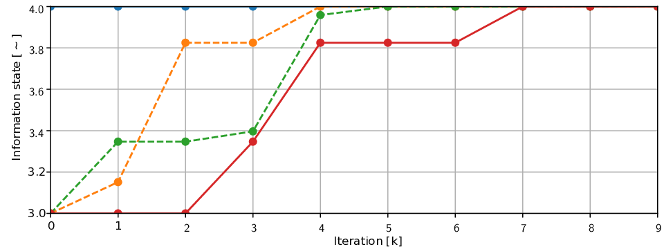
The multi-agent system, with network topology $(\mathcal{N},\mathcal{A})$ as in Figure 1(a) and with identical and constant channel coefficients, is endowed with the switching consensus protocol (50) and the simulation result is shown in Figure 6. Unlike Example 1, finite-time max-consensus is achieved. At instant $k=2T(0)+1=5$ , all non-maximal agents have lost authorization to broadcast; by this, at instant $k=2T(0)+2=6$ , all those agents including a maximal agent in their neighbourhood become maximal as well. In the case of a fading channel, where normalized channel coefficients are as in (15), with channel coefficients drawn out of a Rayleigh distribution with variance $1$ , finite-time max-consensus is also achieved, as shown in Figure 7.

Example 6.

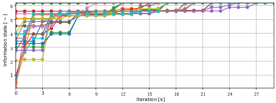
In this example, a larger system is analyzed. The number of agents, the network topology, the channel coefficients, and the initial information state are randomly chosen (under the only constraint that the network topology has to be strongly connected), as shown in Figure 8. Such a system, employed with the switching consensus protocol (50), achieves finite-time max-consensus, as indicated in Figure 9.

IV-D Comparison with the standard approach

In Section II-B, we presented the so-called standard approach. It consists of the combination of an orthogonal channel access communication method and the consensus protocol (6). We now compare the standard approach with the extended protocol (50), to investigate the benefits of the latter.

Fig. 10: Each point comes from a randomized experiment, whose abscissa represents the network size and its whose ordinate is the ratio

\bar{k}_{t}/\bar{k}_{b}

. All points above the red line correspond to those cases when the here proposed max-consensus protocol performs better than the traditional approach.

In the following, the channel access method used for comparison is TDMA (Time-Division Multiple Access); this method guarantees orthogonal transmissions by dividing each discrete transmission into different time slots. Clearly, each iteration considered in (6) then corresponds in reality to $n$ such time slots, since each of the $n$ users has to transmit in a one-after-the-other fashion.

On the other hand, computing inputs for the agents via superposition (cf. (17)) takes $2$ communication time-slots (see Section II-D), independently of the network size, in order to obtain the normalized channel fading coefficients. Yet, consensus protocol (50) requires, in general, a higher number of iterations than the standard approach, and it depends on channel realization. Therefore, a meaningful comparison can be only done via randomized simulations.

For networks of size between $3$ and $100$ , one hundred different simulations are executed. Each one represents a random initial vector and a random (connected) topology. $\forall k\in\mathbb{N}_{0}$ , $\forall i\in\mathcal{N},\ \forall j\in N_{i}(k)$ , the random channel coefficients $\xi_{ij}(k)$ are drawn out of independent Rayleigh distributions with variance $1$ . $\bar{k}_{t}$ denotes the number of time slots required by the traditional approach for achieving max-consensus, and $\bar{k}_{b}$ the number of time-slots required by the switching protocol (50) to ensure max-consensus. For each experiment, in Figure 10, we plot the ratio of the two quantities, defined as $r=\frac{\bar{k}_{t}}{\bar{k}_{b}}$ . The numerical experiment shows that for multi-agent systems composed of more than approximately $15$ agents, employing (50) and channel superposition saves significant convergence time.

V Conclusion

This paper has presented a possible solution for achieving max-consensus in multi-agent systems communicating over real fading wireless channels. First, a suitable communication system has been designed. By employing this strategy, a max-consensus protocol adopting broadcast authorizations has been proven to guarantee asymptotic convergence. Then, this protocol has been extended with a switching protocol guaranteeing finite-time convergence.

Future work will consider the relaxation of some of the assumptions made in the paper. In particular, we will study the case of a noisy channel, and we will investigate the effort of asynchronous broadcasts.

References

[1] Rudolf Ahlswede. Multi-way communication channels. In Second International Symposium on Information Theory: Tsahkadsor, Armenia, USSR, Sept. 2-8, 1971, 1973.
[2] Karl J Åström and Björn Wittenmark. Computer-controlled systems: theory and design. Courier Corporation, 2013.
[3] Igor Bjelaković, Matthias Frey, and Sławomir Stańczak. Distributed approximation of functions over fast fading channels with applications to distributed learning and the max-consensus problem. In 2019 57th Annual Allerton Conference on Communication, Control, and Computing (Allerton), pages 1146–1153. IEEE, 2019.
[4] Luc Brunet, Han-Lim Choi, and Jonathan How. Consensus-based auction approaches for decentralized task assignment. In AIAA guidance, navigation and control conference and exhibit, page 6839, 2008.
[5] Ming Cao, A Stephen Morse, and Brian DO Anderson. Reaching a consensus in a dynamically changing environment: convergence rates, measurement delays, and asynchronous events. SIAM Journal on Control and Optimization, 47(2):601–623, 2008.
[6] Jung Il Choi, Mayank Jain, Kannan Srinivasan, Phil Levis, and Sachin Katti. Achieving single channel, full duplex wireless communication. In Proceedings of the sixteenth annual international conference on Mobile computing and networking, pages 1–12. ACM, 2010.
[7] Thomas M Cover and Joy A Thomas. Elements of information theory. John Wiley & Sons, 2012.
[8] Donato Di Paola, Antonio Petitti, and Alessandro Rizzo. Distributed kalman filtering via node selection in heterogeneous sensor networks. International Journal of Systems Science, 46(14):2572–2583, 2015.
[9] A. Giridhar and P.R. Kumar. Toward a theory of in-network computation in wireless sensor networks. IEEE Communications Magazine, 44(4):98–107, apr 2006.
[10] Mario Goldenbaum, Holger Boche, and Slawomir Stańczak. Nomographic gossiping for f-consensus. In 2012 10th International Symposium on Modeling and Optimization in Mobile, Ad Hoc and Wireless Networks (WiOpt), pages 130–137. IEEE, 2012.
[11] Mario Goldenbaum, Holger Boche, and Sławomir Stańczak. Harnessing interference for analog function computation in wireless sensor networks. IEEE Transactions on Signal Processing, 61(20):4893–4906, 2013.
[12] Mario Goldenbaum and Slawomir Stanczak. Robust analog function computation via wireless multiple-access channels. IEEE Transactions on Communications, 61(9):3863–3877, 2013.
[13] Franck Iutzeler, Philippe Ciblat, and Jérémie Jakubowicz. Analysis of max-consensus algorithms in wireless channels. IEEE Transactions on Signal Processing, 60(11):6103–6107, 2012.
[14] Andreas Kortke, Mario Goldenbaum, and Sławomir Stańczak. Analog computation over the wireless channel: A proof of concept. In SENSORS, 2014 IEEE, pages 1224–1227. IEEE, 2014.
[15] Magni Lalo and Scattolini Riccardo. Advanced and multivariable control. Pitagoga edirice Bologna, 2014.
[16] Vittorio Lippi, Fabio Molinari, and Thomas Seel. Distributed bio-inspired humanoid posture control. 2019.
[17] Fabio Molinari, Alexander Martin Dethof, and Joerg Raisch. Traffic automation in urban road networks using consensus-based auction algorithms for road intersections. 2019 European Control Conference (ECC), 2019.
[18] Fabio Molinari and Jörg Raisch. Efficient consensus-based formation control with discrete-time broadcast updates. In 2019 Conference on Decision and Control (CDC), pages 4172–4177. IEEE, 2019.
[19] Fabio Molinari and Jörg Raisch. Exploiting wireless interference for distributively solving linear equations. In To appear in IFAC World Congress 2020., 2020.
[20] Fabio Molinari, Sławomir Stańczak, and Jörg Raisch. Exploiting the superposition property of wireless communication for average consensus problems in multi-agent systems. European Control Conference, 2018.
[21] Fabio Molinari, Sławomir Stańczak, and Jörg Raisch. Exploiting the superposition property of wireless communication for max-consensus problems in multi-agent systems. IFAC-PapersOnLine, 51(23):176–181, 2018.
[22] Shaoshuai Mou, Ji Liu, and A Stephen Morse. A distributed algorithm for solving a linear algebraic equation. IEEE Transactions on Automatic Control, 60(11):2863–2878, 2015.
[23] Richard M Murray. A mathematical introduction to robotic manipulation. CRC press, 2017.
[24] Behrang Monajemi Nejad, Sid Ahmed Attia, and Jörg Raisch. Max-consensus in a max-plus algebraic setting: The case of fixed communication topologies. In Information, Communication and Automation Technologies, 2009. ICAT 2009. XXII International Symposium on, pages 1–7. IEEE, 2009.
[25] Reza Olfati-Saber. Flocking for multi-agent dynamic systems: Algorithms and theory. Technical report, CALIFORNIA INST OF TECH PASADENA CONTROL AND DYNAMICAL SYSTEMS, 2004.
[26] Reza Olfati-Saber, J Alex Fax, and Richard M Murray. Consensus and cooperation in networked multi-agent systems. Proceedings of the IEEE, 95(1):215–233, 2007.
[27] Wei Ren. Consensus strategies for cooperative control of vehicle formations. IET Control Theory & Applications, 1(2):505–512, 2007.
[28] Wei Ren, Randal W Beard, and Ella M Atkins. Information consensus in multivehicle cooperative control. IEEE Control Systems, 27(2):71–82, 2007.
[29] David Tse and Pramod Viswanath. Fundamentals of Wireless Communication. Cambridge University Press, 2012.
[30] Mathukumalli Vidyasagar. Nonlinear systems analysis, volume 42. Siam, 2002.
[31] Meng Zheng, Mario Goldenbaum, Sławomir Stańczak, and Haibin Yu. Fast average consensus in clustered wireless sensor networks by superposition gossiping. In 2012 IEEE Wireless Communications and Networking Conference (WCNC), pages 1982–1987. IEEE, 2012.