Non-reversible guided Metropolis kernel
Abstract
We construct a class of non-reversible Metropolis kernels as a multivariate extension of the guided-walk kernel proposed by Gustafson 1998. The main idea of our method is to introduce a projection that maps a state space to a totally ordered group. By using Haar measure, we construct a novel Markov kernel termed Haar-mixture kernel, which is of interest in its own right. This is achieved by inducing a topological structure to the totally ordered group. Our proposed method, the -guided Metropolis–Haar kernel, is constructed by using the Haar-mixture kernel as a proposal kernel. The proposed non-reversible kernel is at least times better than the random-walk Metropolis kernel and Hamiltonian Monte Carlo kernel for the logistic regression and a discretely observed stochastic process in terms of effective sample size per second.
1 Introduction
1.1 Non-reversible Metropolis kernel
Markov chain Monte Carlo methods have become essential tools in Bayesian computation. Bayesian statistics has been strongly influenced by the evolution of the methods. This influence is well expressed in Robert and Casella 2011; Green et al 2015. However, the applicability of traditional Markov chain Monte Carlo methods is limited for some statistical problems involving large data sets. This motivated researchers to work on new kinds of Monte Carlo methods, such as piecewise deterministic Monte Carlo methods (Bouchard-Côté et al 2018; Bierkens et al 2019), divide-and-conquer methods (Wang and Dunson 2013; Neiswanger et al 2014; Scott et al 2016), approximate subsampling methods (Welling and Teh 2011; Ma et al 2015), and non-reversible Markov chain Monte Carlo methods.
In this paper, we focus on non-reversible Markov chain Monte Carlo methods. Reversibility refers to the sophisticated balancing condition (detailed-balance condition) which makes the Markov kernel invariant with respect to the probability measure of interest. Although reversible Markov kernels form a nice class (Kipnis and Varadhan 1986; Roberts and Rosenthal 1997; Roberts and Tweedie 2001; Kontoyiannis and Meyn 2011), the condition is not necessary for the invariance. Breaking reversibility sometimes improves the convergence properties of Markov chains (Diaconis and Saloff-Coste 1993; Diaconis et al 2000; Andrieu and Livingstone 2019).
However, without the sophisticated balancing condition, constructing a Markov chain Monte Carlo method is not an easy task. There are many efforts working in this direction but still there are large gaps between the theory and practice. The guided-walk method for probability measures on one-dimension Euclidean space was proposed by Gustafson 1998 which sheds light on this direction. Its multivariate extension has also been studied in Ma et al 2019 but is still based on a one dimensional Markov kernel. In this paper we consider a general multivariate extension of Gustafson 1998, termed guided Metropolis kernel. To do this, we first briefly describe their method.
In the algorithm proposed in Gustafson 1998, a direction variable is attached to each state , which is either the positive direction or the negative direction. If the positive direction is attached, the new proposed state is
| (1.1) |
where is the current value and is the random noise. If the negative direction is attached, the new proposed state is
The proposed state is accepted as the new state with the so-called acceptance probability. If the proposed state is accepted, the new state is assigned the same direction as the previous state. Otherwise, the opposite direction is assigned to the new state, and the new state is same as the previous state.
If we want to generalise this procedure to a more general state space, say , we may need to interpret the summation operator in (1.1) differently, since, for example, is not closed with the operation. So we have to find a state space that has a suitable summation operator, in other words, a group structure. For this reason, we consider an abstract setting throughout in this paper, as this is the most natural way to describe our setting and algorithms.
More precisely, the main idea of our method is to introduce a projection which maps a state space to a totally ordered group. By this ordering we will decompose any Markov kernel into a sum of positive () and negative () directional sub Markov kernels. By using rejection sampling, two sub Markov kernels are normalised to be positive and negative Markov kernels. Then we can construct a non-reversible Markov kernel on by the systematic-scan Gibbs sampler. Similar ideas can be found in Gagnon and Maire 2020 for a discrete state space case.
Usually, total masses of sub Markov kernels are quite different which results in inefficiency of rejection sampling. To avoid this issue, we focus on the case where the total masses are the same. However, it is non trivial to find such a Markov kernel. By using Haar measure, we introduce a novel Markov kernel termed Haar-mixture kernel, that has this property. This is achieved by introducing a topological structure to the totally ordered group and . Our proposed method, the -guided Metropolis–Haar kernel, is constructed by using the Haar-mixture kernel as a proposal kernel. By using this, we introduce many non-reversible -guided Metropolis–Haar kernels which are of practical interest.
1.2 Literature review
Here we briefly review the existing literature which has studied non-reversible Markov kernels that modify reversible Metropolis kernels. First of all, products of reversible Markov kernels are not reversible in general. For example, the systematic-scan Gibbs sampler is usually non-reversible.
The so-called lifting method was considered in, for example, Diaconis et al 2000; Turitsyn et al 2011; Vucelja 2016; Gagnon and Maire 2020. In this method, a Markov kernel is lifted to an augmented state space by splitting the Markov kernel into two sub-Markov kernels. An auxiliary variable chooses which kernel should be followed. The guided-walk kernel (Gustafson 1998) and the method we are proposing are classified into this category. Another approach is preparing two Markov kernels in advance and constructing a systematic-scan Gibbs sampler as in Ma et al 2019.
The Hamiltonian Monte Carlo kernel has an auxiliary variable by construction. Therefore, a systematic-scan Gibbs sampler can naturally be defined, as in Horowitz 1991. Also, Tripuraneni et al 2017 constructed a different non-reversible kernel which twists the original Hamiltonian Monte Carlo kernel. See also Sherlock and Thiery 2017; Ludkin and Sherlock 2019.
An important exception that does not introduce an auxiliary variable is Bierkens 2016 that introduces an anti-symmetric part into the acceptance probability so that the kernel becomes non-reversible while preserving -invariance, where a Markov kernel is called -invariant if . See also Neal 2020 that avoids requiring an additional auxiliary variable by focusing on the uniform distribution that is implicitly used for the acceptance-rejection procedure in the Metropolis algorithm.
In this paper, non-reversible Markov kernels are designed using the Haar measure. The use of the Haar measure in the Monte Carlo context is not new. Liu and Wu 1999 used the Haar measure to improve the convergence speed of the Gibbs sampler, which was further developed by Liu and Sabatti 2000; Hobert and Marchev 2008. Also, the Haar measure is a popular choice of prior distribution in the Bayesian context (Berger 1993; Robert 2007; Ghosh et al 2006). Markov chain Monte Carlo methods with models using the prior distribution are naturally related to the Haar measure.
1.3 Construction of the paper
The main objective of this paper is to present a framework for the construction of a class of non-reversible kernels, which are described in Section 4. Sections 2 and 3 are devoted to introducing some useful ideas for the construction of the non-reversible kernels.
Section 2.1 contains an introduction to some reversible kernels, such as the convolution-type construction of reversible kernels and Metropolis kernels. In Section 2.2, we introduce the Haar-mixture kernel and the Metropolis–Haar kernel. The Metropolis–Haar kernel is useful in its own right, although it does not have non-reversible property. Moreover, it is actually a key Markov kernel for non-reversible kernels. However, the connection to non-reversible kernels is explained in Section 3 rather than Section 2.
In Section 3 we introduce three properties, unbiasedness, random-walk, and sufficiency properties. These properties are introduced from Section 3.1 to Section 3.3 sequentially. As described in Section 1.1, our construction of the non-reversible kernel is based on a Markov kernel that generates a state in the positive and negative directions with equal probability. This property is referred to as unbiasedness in Section 3.1 which is the sufficient condition for constructing non-reversible kernels. In Section 3.2, we introduced a more specific form of the unbiasedness property, the random-walk property. In Section 3.3, we introduce the sufficiency property to describe a specific form of the random-walk property using the Haar-mixture kernel introduced in Section 2.2. Section 3.4 describes how to generalise a one-dimensional unbiased kernel to a multivariate kernel.
Section 4 is the section for non-reversible kernels. In Section 4.1 we introduce a class of non-reversible kernels, the -guided Metropolis kernel. We focus on the -guided Metropolis–Haar kernel, which is a -guided Metropolis kernel using Haar-mixture kernel. In Section 4.2, we show step-by-step instructions for constructing -guided Metropolis–Haar kernels. Some examples can be found in Section 4.3.
1.4 Some group related concepts
A set is a totally ordered set if it has a binary relation which satisfies three properties:
- •
and implies ,
- •
if and , then ,
- •
or for all .
We call an order relation. The totally ordered set can be equipped with the order topology induced by and for . A Borel -algebra is generated from the order topology.
A group is an ordered group if there is an order relation such that
| (1.2) |
for .
A group with a topology on is called a topological group if its group actions and are continuous. If is locally compact and Hausdorff, it is called a locally compact topological group. For any locally compact topological group, there is a left and right Haar measures. The group is called unimodular if the left Haar measure and the right Haar measure coincide up to a multiplicative constant. See Halmos 1950 for the detail.
The set is a left -set, if there exists a left-group action from to such that and where is the identity and . We denote for . In this paper, any map is called a statistic when is a totally ordered set. A statistic is called a -statistic if for and and if is an ordered group.
2 Haar-mixture kernel
2.1 Reversibility and Metropolis kernel
Before analysing the non-reversible Markov kernel, we first recall the definition of reversibility. Reversibility is important throughout the paper since our construction of a non-reversible Markov kernel is based on classes of reversible Markov kernels. A Markov kernel on a measurable space is -reversible for a -finite measure if
| (2.1) |
for any . If is -reversible, then is -invariant. There is a strong connection between ergodicity and -reversibility. See Kipnis and Varadhan 1986; Roberts and Rosenthal 1997; Roberts and Tweedie 2001; Kontoyiannis and Meyn 2011.
As we mentioned above, our non-reversible Markov kernel is based on a class of reversible kernels. Suppose that is a probability measure on where is closed by a summation operator. A simple approach to construct a reversible kernel is to first describe as an image measure of a convolution of probability measures under a measurable map , i.e., . Here, an image measure of a measure under a map is defined by
and a convolution of and is defined by
where . Then define independent random variables and . Finally, construct as the conditional distribution of given . Then the probabilities in (2.1) are and which are the same by construction. We refer to this as the convolution-type construction.
Let . Let be the -identity matrix.
Example 2.1 (Autoregressive kernel).
We first describe the well-known autoregressive kernel resulting from the above convolution-type construction. Let and be a positive definite symmetric matrix, and let . Further, let be the normal distribution with mean and covariance matrix . By the reproductive property of the normal distribution, is a convolution of probability measures and with in the notation above. Then the random variable and in the above notation follow with covariance
By the change-of-variables formula, the conditional distribution is the autoregressive kernel, which is defined as
Due to the nature of convolution, it is -reversible.
Example 2.2 (Beta-Gamma kernel).
Let be the Gamma distribution with shape parameter and rate parameter . Let , and and where and . The conditional distribution of given in the notation above, is , where is the Beta distribution with shape parameters and . Therefore, the conditional distribution on , called Beta-Gamma (autoregressive) kernel in this paper, is given by
where are independent, and corresponds to in the above notation. The kernel is -reversible by construction. See Lewis et al 1989.
Example 2.3 (Chi-squared kernel).
We construct a -reversible kernel for . Let and and . By the reproductive property, if and then . Therefore, since is the Chi-squared distribution with -degrees of freedom. The conditional distribution is -reversible by construction. We show that the conditional distribution is given by
| (2.2) |
where are independent and follow the standard normal distribution. To see this, first note that the law of given is . Then the law of given is the non-central Chi-squared distribution with -degrees of freedom and the non-central parameter . The expression (2.2) follows from the property of the non-central Chi-squared distribution.
The Metropolis algorithm is a clever way to construct a reversible Markov kernel with respect to a given probability measure, . The following definition is somewhat broader than the usual one. It even includes the independent Metropolis–Hastings kernel, which is usually classified as a Metropolis–Hastings kernel and not a Metropolis kernel. An important feature of this kernel compared to the more general Metropolis–Hastings kernel is that we do not need to know the explicit density function of the proposed Markov kernel .
Definition 2.4 (Metropolis kernel).
Let be a measure, and let be a probability measure with probability density function respect to . Let be a -reversible Markov kernel. A Markov kernel is called a Metropolis kernel of if
for
| (2.3) |
The function is called the acceptance probability, and Markov kernel is called the proposal kernel.
2.2 Haar-mixture kernel
We introduce Markov kernels using the Haar measure. The Haar measure enables us to construct a random walk on a locally compact topological group, which is a crucial step towards obtaining non-reversible Markov kernels in this paper. The connection between the Markov kernels and the random walk will be made clear in Section 3, and the connection with non-reversible Markov kenrels will be clear in Section 4.
The idea of constructing Haar-mixture kernels is to introduce an auxiliary variable corresponding to the scaling parameter or the shift parameter of the state space. We set a prior distribution on . In each iteration of the random number generation, the parameter is generated from the conditional distribution given the state space using the prior distribution. The Haar-mixture kernel uses the Haar measure for the prior distribution of . As commented above, the reason for using the Haar measure will be made clear in later sections.
Let be a locally compact topological group equipped with the Borel -algebra. Let be a left -set. We assume that is equipped with a -algebra and the left-group action is jointly measurable. Let be a -reversible Markov kernel on , where is a -finite measure. Let
where . Then is -reversible where
Let be the right Haar measure on . It satisfies and where . Set
| (2.4) |
Assume that is a -finite measure. Then is a left-invariant measure. Indeed,
Suppose that is absolutely continuous with respect to . Then is jointly measurable. This is because by the left-invariance of , and is assumed to be jointly measurable. Let
| (2.5) |
By the Radon–Nikodým theorem, -almost surely. Define
| (2.6) |
Definition 2.5 (Haar-mixture kernel).
The Markov kernel defined by (2.6) is called the Haar-mixture kernel of .
Example 2.6 (Autoregressive mixture kernel).
Consider the autoregressive kernel in Example 2.1. Let and , and set . Then the Haar measure is . A simple calculation yields and . Also, and where . We have a closed form (up to a constant) of expression of as follows:
Example 2.7 (Beta-Gamma mixture kernel).
For the Beta-Gamma kernel in Example 2.2, we introduce the operation with . By this operation, is a left -set. We have , and the Markov kernel is the same as replacing by . The Haar measure on is , and hence and .
Example 2.8 (Chi-squared mixture kernel).
For the Chi-squared kernel in Example 2.3, let , and set . We have , and the Markov kernel is the same as replacing the standard normal distribution by . The Haar measure is . In this case, , and .
Proposition 2.9.
The Haar-mixture kernel is -reversible.
Proof.
Let . Since is -reversible,
∎
From this, we can define the following Metropolis kernel.
Definition 2.10 (Metropolis–Haar kernel).
A Metropolis kernel of is called a Metropolis–Haar kernel if is a Haar-mixture kernel.
The Metropolis–Haar kernel is implemented as the following algorithm, where . In the algorithm, is the uniform distribution on .
The Metropolis–Haar kernel is reversible, but important in its own right. The underlying reference measure is heavier than , which is expected to lead to a robust algorithm. Examples of Metropolis–Haar kernels will be described in Section 4.3.
3 Unbiasedness, the random-walk property and sufficiency
3.1 Unbiasedness
In this section, we introduce the unbiasedness property for efficient construction of the non-reversible kernel. Any measurable map is called a statistic in this paper, where is a totally ordered set. In Section 4, a statistic will guide a Markov kernel according to the auxiliary directional variable as in Gustafson 1998. When the positive direction is selected, then is sampled according to unless by rejection sampling. If the negative direction is selected, is sampled unless . It is typical that one of the rejection sampling directions has high rejection probability (see Example 3.2). To avoid this inefficiency, we consider a class of Markov kernels such that the probabilities of the events and measured by are the same. We say is unbiased if this property is satisfied. If the unbiasedness is violated, the rejection sampling can be inefficient because it takes a long time to exit the while loop of the rejection sampling. Therefore, the unbiasness property is necessary for efficient construction of the nonreversible kernel in our approach.
Definition 3.1 (-unbiasedness).
Let be a statistic. We say a Markov kernel on is -unbiased if
for any . Also, we say that two statistics and from to possibly different totally ordered sets are equivalent if
for , where .
If and are equivalent, then -unbiasedness implies -unbiasedness.
Example 3.2 (Random-walk kernel).
Let be the transpose of and be a probability measure on which is symmetric about the origin, that is, for . Let . Then is -unbiased for for some since
On the other hand, is not -unbiased for , where , if is not the Dirac measure centred on . In particular, if , then for .
3.2 Random-walk property
Constructing a -unbiased Markov kernel is a crucial step for our approach. However, determining how to construct a -unbiased Markov kernel is nontrivial. The random-walk property is the key for this construction.
Let be a topological group.
Definition 3.3 (-random-walk).
A Markov kernel has the -random-walk property if there is a function with a probability measure on a topological group such that for any Borel set of and
| (3.1) |
Here, .
A typical example of a Markov kernel with the -random-walk property is Example 3.2. We assume that is an ordered group.
Proposition 3.4.
If has the -random-walk property, then is -unbiased.
Proof.
Let . Then for the unit element ,
Similarly, . Since , is -unbiased. ∎
3.3 Sufficiency
So far in this section, we have introduced the -unbiasedness, which is the important property for the -guided Metropolis kernel in Section 3.1. In Section 3.2, we showed that the -random-walk property is sufficient for the -unbiasedness. In this subsection we will show that for the Haar-mixture kernel, the sufficiency property introduced below is sufficient for the -random-walk property, and for the -unbiasedness property.
We would like to mention the intuition behind the sufficiency property. In general, the conditional law of given is not completely determined by . If it is completely determined by , we call sufficient. If is sufficient, the equation (3.1) is satisfied, although is not symmetric in general. When is the Haar mixture kernel with some additional technical conditions, we will show that is symmetric thanks to the Haar measure property.
Let be a unimodular locally compact topological group. Also, let be an ordered group, be a left -set. In this paper, a statistics is called a -statistics if for and . For a -finite measure on and a -statistic , let , that is, the image measure of under . Let be the image measure of under . Then it is a left Haar measure, since
by the left-invariance of . Since is unimodular, the left Haar measure and right Haar measure coincide up to a multiplicative constant. From this fact, we can assume
without loss of generality. Let be a -reversible kernel.
Definition 3.5 (Sufficiency).
Let be a -finite measure. We call a -statistic sufficient if there is a Markov kernel and a measurable function on such that
and
-almost surely.
By the left-invariance of , we have
| (3.2) |
since
Let be the image measure of under . Then is -reversible and
Example 3.6 (Sufficiency of the Autoregressive mixture kernel).
Consider the Autoregressive kernel in Example 2.1 and the statistics defined in Example 2.6. We show that is sufficient for . The Markov kernel corresponds to the update
where . For ,
where is the Euclidean norm. Therefore, conditioned on follows the non-central Chi-squared distribution with degrees of freedom and non-central parameter . Hence, the law of depends on only through and hence there exists a Markov kernel as in Definition 3.5. Also, a simple calculation yields . Therefore, is sufficient for .
Example 3.7 (Sufficiency of the Beta-Gamma and Chi-squared kernels).
For a measure , we write for the th product of defined by
for .
Proposition 3.8.
Suppose a -statistic is sufficient for a -reversible kernel . Also, suppose a probability measure on is absolutely continuous with respect to . Then has the -random-walk property for a probability measure . In particular, it is -unbiased.
Proof.
Let be the Radon–Nikodým derivative:
By the -reversibility of , almost surely. From the sufficiency property, we can rewrite and by and :
-almost. Together with (3.2), we have
where the last equality follows from the right-invariance of . Let
From ,
By using , we can write
The above is guaranteed to have the -random-walk property by introducing because
and
Hence, it is -unbiased by Proposition 3.4. ∎
3.4 Multivariate version of one-dimensional kernels
Essentially, we have introduced three Markov kernels, the Autoregressive kernel, the Chi-squared kernel, and the Beta-Gamma kernel. The state space of the first kernel is a general Euclidean space and that of the last two kernels is a subspace of the one-dimensional Euclidean space. In this subsection, we consider the multivariate version of the latter two kernels.
We present different strategies for the two kernels. For the Chi-squared kernel, there is a sophisticated structure that allows multivariate version of the state space. For the Beta-Gamma kernel, there does not seem to have a special structure and so we apply a general approach which does not require any structure. First we show how to construct a multivariate extension for the Chi-squared kernel.
Example 3.9 (Multivariate Chi-squared mixture kernel).
For the Chi-squared kernel (Examples 2.3, 2.8), we use the operation with and . Let be the Markov kernel defined in Example 2.3. Let
and . Let . In this case, and , and on is the product of on defined in Example 2.8, that is,
Then
and . From this expression, . Moreover, by the property of the non-central Chi-squared distribution, the law of where is the non-central Chi-squared distribution with -degrees of freedom with the non-central parameter . Therefore there exists a Markov kernel which is the scaled non-central Chi-squared distribution for each . Obviously, it has a density function with respect to . The statistic is sufficient and the multivariate version of Chi-squared mixture kernel is -unbiased from this fact.
Example 3.10 (Multivariate Beta-Gamma mixture kernel).
For the Beta-Gamma kernel (Examples 2.2, 2.7), we use the operation with and where and . We define the binary operation of by and the identity element by . In this case, the Markov kernel on is the product of on defined in Example 2.7, that is,
Also, we have and . The -statistic is sufficient, and hence the Multivariate version of Beta-Gamma mixture kernel is -unbiased by Proposition 3.8.
For in Example 3.10, several types of order relations are possible. Any ordering will do as long as (1.2) is satisfied. The popular lexicographic order depends on how we index the coordinates. To avoid this unfavourable property, we consider the modified lexicographic order defined below.
Example 3.11 (Modified lexicographical order).
Let . For , let
be a partial product of the vector from the th element to the th element. A version of lexicographical order can be defined as follows. Counting from ,
- •
if for all or
- •
if the first index such that satisfies ,
then we write . It is not difficult to check that this ordering satisfies (1.2).
Since (1.2) is satisfied, the multivariate Beta-Gamma mixture kernel is -unbiased with this order for . Note that the modified lexicographic order also has the same problem as that of the (un-modified) lexicographic order, that is, it depends how we index the coordinate. However, the problem occurs with probability . This is because the first step of the sort (i.e. or ) does not depend on the order of the indexes and the first step determines the order with probability . More precisely,
with the modified lexicographical ordering and
in with usual ordering are equivalent in the sense of Definition 3.1 because . In particular, the multivariate Beta-Gamma mixture kernel is -unbiased since the kernel is -unbiased. Note that is not a -statistic, since it does not satisfy .
4 Guided Metropolis kernel
4.1 -Guided Metropolis kernel
Definition 4.1 (-guided Metropolis kernel).
For -unbiased Markov kernel , probability measure and a measurable function defined in (2.3), we say a Markov kernel on is the -guided Metropolis kernel of if
where
The Markov kernel satisfies the so-called -skew-reversible property
where
Here, for a probability measures and , . With this property, it is straightforward to check that is -invariant.
Example 4.2 (Guided-walk kernel).
The -guided Metropolis kernel corresponding to the random-walk kernel on is called the guided-walk in Gustafson 1998. For a multivariate target distribution, for some was considered in Gustafson 1998; Ma et al 2019.
As described in Proposition 3.8, a Haar mixture kernel is -unbiased if is sufficient and some other technical conditions are satisfied. Therefore, we can construct a -guided Metropolis kernel using the Haar mixture kernel .
Definition 4.3 (-guided Metropolis–Haar kernel).
If a Haar-mixture kernel is -unbiased, the -guided Metropolis kernel of is called the -guided Metropolis–Haar kernel.
The -guided Metropolis–Haar kernel is given as Algorithm 2, where we let . This Metropolis–Haar kernels is further discussed in detail in Sections 4.2 and 4.3.
Let be the Metropolis kernel of . We now see that is always expected to be better than in the sense of the asymptotic variance corresponding to the central limit theorem. The inner product and the norm can be defined on the space of -square integrable functions. Let be a Markov chain with Markov kernel and . Then we define the asymptotic variance
if the right-hand side exists. The existence of the right-hand side limit is a kernel-specific problem and not addressed here. Let . As in Andrieu 2016, to avoid a kernel-specific argument, we consider a pseudo asymptotic variance
where , which always exists. Under some conditions, . We can also define for -square integrable function on by considering .
Proposition 4.4 (Theorem 3.17 of Andrieu and Livingstone 2019).
Suppose that is -square integrable. Then for , .
By taking , we can expect that the non-reversible kernel is better than in the sense of smaller asymptotic variance.
4.2 Step-by-step instruction for creating a -guided Metropolis–Haar kernel
Here is a set of necessary conditions to build a Haar-mixture kernel and a Metropolis–Haar kernel .
- 1.
is a locally compact topological group equipped with the Borel -algebra and the right Haar measure .
- 2.
State space is a left -set.
- 3.
is a -finite measure and is -reversible Markov kernel on .
- 4.
There exists a Markov kernel as in (2.5).
Then we can construct a Haar–mixture kernel as in (2.6). Here is an additional set of necessary conditions to build a -guided Metropolis–Haar kernel.
- 1.
is an ordered group, and is a unimodular locally compact topological group.
- 2.
is a -statistics.
- 3.
is sufficient for .
4.3 Examples of -guided Metropolis–Haar kernels
Here we present some of the -guided Metropolis–Haar kernels.
Example 4.5 (Guided Metropolis autoregressive mixture kernel).
The Metropolis kernel of with the proposal kernel defined in Example 2.1 is called the preconditioned Crank–Nicolson kernel. This kernel was studied in Neal 1999; Beskos et al 2008; Cotter et al 2013. The Metropolis–Haar kernel with the Haar-mixture kernel in Example 2.6 is called the mixed preconditioned Crank–Nicolson kernel. This kernel was developed in Kamatani 2017; Kamatani 2018. The -guided Metropolis–Haar kernel of with and , called the -guided mixed preconditioned Crank–Nicolson kernel, can be constructed as in Definition 4.1. In this case, for a constant and a symmetric positive definite matrix , , and and . We can perform the -guided Metropolis–Haar kernel as in Algorithm 2.
Example 4.6 (Guided Metropolis Multivariate Beta-Gamma mixture kernel).
The Metropolis kernel of and the Metropolis–Haar kernel of in Example 3.10 can be defined naturally, and the former kernel was studied in Hosseini 2019. The -guided Metropolis–Haar kernel with is constructed by , and as in Example 3.10. In this case, .
5 Simulation
5.1 -guided Metropolis–Haar kernel on
In this simulation, we consider the autoregressive based kernel considered in Example 4.5. More precisely, we study the preconditioned Crank–Nicolson kernel, the mixed-preconditioned Crank–Nicolson kernel and the -guided mixed preconditioned Crank–Nicolson kernel. The random-walk Metropolis kernel is also compared for a reference. All these methods are gradient-free, information blind methods in the sense that the proposal kernel does not use the derivative of . Although this may sound daunting, sometimes a simple structure leads to robustness and efficiency as described through simulation experiments. Moreover, parameter tuning for these Markov kernels based on a reversible proposal kernel is relatively straightforward. We can learn the parameters of the reference measures or using the standard technique of treating the MCMC outputs as if they were from identically and independent observations of or , even though is generally improper distribution. Since parameter tuning is not our main focus, we do not elaborate on this point in this paper.
We also compare these methods with gradient based, informed algorithms. The Metropolis-adjusted Langevin algorithm (Rossky et al 1978; Roberts and Tweedie 1996) and the Hamiltonian Monte Carlo algorithm (Duane et al 1987; Neal 2011) are popular gradient based algorithms. Furthermore, we consider the methods that use both gradient-based and autoregressive kernel based ideas. This class includes such as the infinite dimensional Metropolis-adjusted Langevin algorithm (Beskos et al 2008; Cotter et al 2013), a marginal sampler proposed in (Titsias and Papaspiliopoulos 2018), which we will refer to the marginal gradient-based sampling, and the infinite dimensional Hamiltonian Monte Carlo (Neal 2011; Ottobre et al 2016; Beskos et al 2017).
We performed all experiments using a desktop computer with 6 cores Intel i7-5930K (3.50GHz) CPU. All algorithms other than the Hamilton Monte Carlo algorithm were coded in R version 3.6.3 (R Core Team 2020) using the RcppArmadillo package version 0.9.850.1.0 (Eddelbuettel and Sanderson 2014). The results for the Hamilton Monte Carlo algorithm were obtained using rstan version 2.19.3 (Stan Development Team 2020). For a fair comparison, we use a single core and chain for rstan. The code for all experiments is available in the online repository at the link https://github.com/Xiaolin-Song/Non-reversible-guided-Metropolis-kernel/.
5.1.1 Discrete observation of stochastic diffusion process
First we consider a problem which is difficult to apply gradient based Markov chain Monte Carlo methodologies due to high cost of derivative calculation. Let . Suppose that is a solution process of a stochastic differential equation
where is the -dimensional standard Wiener process and and are the drift and diffusion coefficient respectively. We only observe where and .
We consider a Bayesian inference based on the local Gaussian approximate likelihood since explicit form of the probability density function is not available in general. The local Gaussian approximation approach, including simple least square estimate approach, has been studied in such as Prakasa Rao 1983; Prakasa Rao 1988; Florens-zmirou 1989; Yoshida 1992. See also Beskos et al 2006; Beskos et al 2009 for non-local Gaussian approach based on unbiased estimate of the likelihood.
We consider a Bayesian inference for using local Gaussian approximated likelihood. We set the diffusion coefficient to be , and the drift coefficient to be
where where here is the probability density function with respect to the Lebesgue measure. See Kotz and Nadarajah 2004. Here is generated from a Wishart distribution with -degrees of freedom and the identity matrix as the scale matrix. The terminal time is and the number of observation is . The prior distribution is a normal distribution .
| rwm | Random-walk Metropolis |
|---|---|
| pcn | Preconditioned Crank–Nicolson |
| mpcn | Mixed preconditioned Crank–Nicolson |
| gmpcn | -guided mixed preconditioned Crank–Nicolson |
| mala | Metropolis-adjusted Langevin |
| -mala | Infinite dimensional Metropolis-adjusted Langevin |
| mgrad | Marginal gradient-based sampling |
| hmc | Hamiltonian Monte Carlo via rstan |
| -hmc | Infinite dimensional Hamiltonian Monte Carlo |

The Markov kernels used in this simulation is listed in Table 1. The first four kernels in the table are gradient-free, information blind kernels. The last five kernels are gradient based, informed kernels. All kernels other than the 1st, 5th and 8th algorithms in Table 1 use the prior distribution as the reference distribution. Reference measure here means that the proposal kernel itself is reversible with respect to the measure, or the proposal kernel approximates another Markov kernel that is reversible with respect to the measure.
We apply the Markov chain Monte Carlo algorithms by a 2-step procedure. In the first stage, we run the random-walk Metropolis algorithm as a burn-in stage. For Gaussian reference kernels, is estimated by the empirical mean in the burn-in stage. After the burn-in, we run each algorithm. The result was presented in Table 1 and Figure 2. In this example, the covariance matrix is not preconditioned; we use the prior’s covariance matrix instead.
The acceptance rates for the first two algorithms in Table 1 were set at . For the 3rd and 4th algorithms, acceptance rates were set to to . As suggested by Roberts and Rosenthal 1998 and Titsias and Papaspiliopoulos 2018, the 5th through 7th algorithms, the acceptance probabilities were set to approximately . The 8th algorithm was tuned in two steps. First, we set the number of leapfrog steps to and tune the leapfrog step size so that the acceptance rate is between and according to Beskos et al 2013. Then we increase the number of leapfrog steps until the time-noramlised effective sample size decreases. The tuning parameters of the Hamiltonian Monte Carlo algorithm were controlled using rstan package. As a quantitative measure of efficiency, we used the effective sample size of log-likelihood per second. It was estimated using the package coda in R (Plummer et al 2006).
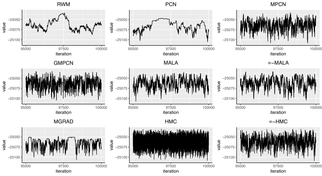
The effective log-likelihood sample sizes per second are shown in Figure 1. The box plot is constructed by fifty independent simulations for each algorithm. The 5th to 7th algorithms, which are Langevin diffusion based algorithms, show the worst performance. Due to the high cost of derivative evaluation, the Hamiltonian Monte Carlo and the infinite dimensional Hamiltonian Monte Carlo are still worse than the random-walk Metropolis kernel. The random-walk Metropolis kernel and the preconditioned Crank–Nicolson kernel are better than gradient-based kernels, but the mixed preconditioned Crank–Nicolson kernel is much better. The -guided version is even better than the non--guided version thanks to the non-reversible property. A trace plot is also shown in the Figure 4, it illustrates that the Hamilton Monte Carlo method has a good performance per iteration, but the cost is high compared to other algorithms.


5.1.2 Logistic regression
Next we apply them to a logistic regression model with the Sonar data set from the University of California, Irvine repository (Dua and Graff 2017). The data set contains 208 observations and 60 explanatory variables. The prior distribution is for each parameters. We use a relatively large variance of the normal distribution because we did not have enough prior information at this stage.
Estimation of the preconditioning matrix is necessary for this problem due to the existence of a strong correlation between the variables. We performed iterations to estimate and estimate the preconditioning matrix using the empirical means. Then we ran iterations for each algorithm, discarding the iterations as burn-in. Furthermore, we ran each experiment for 50 times using different seeds. We evaluate the effective sample size of log-likelihood per second, and present the results of all the algorithms by boxplots (Figure 3). The algorithms based on the Lebesgue measure (1, 5, 8th algorithms in Table 1) are relatively worse than other algorithms based on the Gaussian reference measure. The performances of the gradient-based algorithms are divergent, which might reflect the sensitivity of the gradient-based algorithms, which is well described in the Chopin and Ridgway 2017. In particular, the infinite dimensional Hamiltonian Monte Carlo algorithm shows the better performance in this case, although it shows poor performance in the previous simulation. The -guided mixed preconditioned Crank–Nicolson kernel was slightly worse than infinite dimensional Hamiltonian Monte Carlo algorithm and better than all other algorithms. The Metropolis–Haar and -guided Metropolis–Haar kernels show good and robust results for the two simulation experiments.
We also investigate the sensitivity of the gradient-based algorithms for the same model as displayed in Figure 4. In this example, initial values are randomly generated from a multivariate normal distribution for each algorithm. The number of iteration of each algorithm is . The paths of the gradient-based algorithms depend strongly on the initial values with the exception of the infinite dimensional Hamiltonian Monte Carlo algorithm.
5.1.3 Sensitivity of the choice of
To illustrate the importance of , we additionally run a numerical experiment on a -dimensional multivariate central -distribution with degrees of freedom and identity covariance matrix (Kotz and Nadarajah 2004, 1p). The first element of is and all the other elements are set to be zero. When is large, then the direction is less important for increasing or decreasing the likelihood. We run the algorithms on the target distribution for iterations. The experiment showed that the benefit of non-reversibility diminishes as the importance of the direction shrinks (Table 2).
| mpcn | 378.19 | 96.23 | 94.74 | 93.52 | 95.33 | 46.31 |
| gmpcn | 4245.43 | 116.29 | 114.78 | 115.2 | 117.20 | 40.20 |
5.2 -guided Metropolis–Haar kernels on
Next, we consider the Beta-Gamma based kernels considered in Example 4.6 and the Chi-squared based kernels considered in example 4.7 with . Thus, we consider a total of six Markov kernels. These are the Metropolis kernel, the Metropolis–Haar kernel, and the -guided Metropolis–Haar kernel for each of the Beta-Gamma based and Chi-squared based kernels.
Our goal is not to compare the Beta-Gamma based kernels and the Chi-squared based kernels, but to compare the guided kernels and the non-guided kernels. In this simulation, we illustrate the difference in behaviour between the guided Metropolis kernel and other kernels by plotting trajectories in two dimensions.
We consider a Poisson hierarchical model of the form
where is the observation. In our simulations we set and . The number of unknown parameters is in this case. The parameter has a closed form conditional distribution
Therefore we can use the Gibbs sampler for generating the parameter . On the other hand, since the conditional distribution of is complicated, we apply Monte Carlo algorithms mentioned above. We created two-dimensional trajectory plots to illustrate the difference in behavior between the Metropolis–Haar kernel and its -guided version. The tuning parameters are chosen so that the average acceptance probabilities are – in iterations. Figure 5 shows the trace plots of the last iterations for the kernels. One can clearly see the larger variation for the guided kernels. Thanks to the incident variables, the guided kernel maintains its direction when the proposed value is accepted. The property of maintaining direction has greatly contributed to the increase in variability.
| mh | Metropolis |
| mhh | Metropolis with Haar-mixture kernel |
| gmh | Guided Metropolis |

6 Discussion
The theory and application of non-reversible Markov kernels have been under active development recently, but there still exists a gap between the two. In order to close this gap, we have described how to construct a non-reversible Metropolis kernel on a general state space. We believe that the method we propose can make non-reversible kernels more attractive.
As a by-product, we have constructed the Metropolis–Haar kernel. The Haar-mixture kernel imposes a new state globally by using the random walk on a group, whereas other recent Markov chain Monte Carlo methods use local topological information derived from target densities. We believe that this sheds new light on the proposed gradient-free, global topological approach. A combination of the global and local (gradient-based) approaches is an area of further research.
In this paper, we have not discussed geometric ergodicity, although ergodicity is clear under appropriate regularity conditions. A popular approach for proving geometric ergodicity is based on the establishment of a Foster-Lyapunov-type drift condition, which requires kernel-specific arguments. On the other hand, our motivation is to build a general framework for the non-reversible Metropolis kernels. Therefore, we did not focus on geometric ergodicity. A more in-depth study should be carried out in that direction. See Kamatani 2017 for geometric ergodicity of the mixed preconditioned Crank–Nicolson kernel.
Finally, we would like to remark that the -guided Metropolis–Haar kernel is not limited to or . It is possible to construct the kernel on the -matrix space and the symmetric positive definite matrix space, where are any positive integers. -guided Metropolis–Haar kernels for other state spaces are future work.
Acknowledgements
Kamatani is supported by JSPS KAKENHI Grant Number 20H04149 and JST CREST Grant Number JPMJCR14D7. Song is supported by the Ichikawa International Scholarship Foundation. We thank Sam Power for helpful comments.
References
- Andrieu (2016) Andrieu C (2016) On random- and systematic-scan samplers. Biometrika 103(3):719–726, DOI 10.1093/biomet/asw019, URL https://doi.org/10.1093/biomet/asw019
- Andrieu and Livingstone (2019) Andrieu C, Livingstone S (2019) Peskun-tierney ordering for markov chain and process monte carlo: beyond the reversible scenario. 1906.06197
- Berger (1993) Berger JO (1993) Statistical decision theory and Bayesian analysis. Springer Series in Statistics, Springer-Verlag, New York, corrected reprint of the second (1985) edition
- Beskos et al (2006) Beskos A, Papaspiliopoulos O, Roberts GO, Fearnhead P (2006) Exact and computationally efficient likelihood-based estimation for discretely observed diffusion processes (with discussion). Journal of the Royal Statistical Society: Series B (Statistical Methodology) 68(3):333–382
- Beskos et al (2008) Beskos A, Roberts G, Stuart A, Voss J (2008) MCMC methods for diffusion bridges. Stoch Dyn 8(3):319–350, DOI 10.1142/S0219493708002378, URL http://dx.doi.org/10.1142/S0219493708002378
- Beskos et al (2009) Beskos A, Papaspiliopoulos O, Roberts G (2009) Monte carlo maximum likelihood estimation for discretely observed diffusion processes. The Annals of Statistics 37(1):223–245, DOI 10.1214/07-aos550, URL http://dx.doi.org/10.1214/07-AOS550
- Beskos et al (2013) Beskos A, Pillai N, Roberts G, Sanz-Serna JM, Stuart A (2013) Optimal tuning of the hybrid monte carlo algorithm. Bernoulli 19(5A):1501–1534, DOI 10.3150/12-bej414, URL https://doi.org/10.3150%2F12-bej414
- Beskos et al (2017) Beskos A, Girolami M, Lan S, Farrell PE, Stuart AM (2017) Geometric mcmc for infinite-dimensional inverse problems. Journal of Computational Physics 335:327 – 351, DOI https://doi.org/10.1016/j.jcp.2016.12.041, URL http://www.sciencedirect.com/science/article/pii/S0021999116307033
- Bierkens (2016) Bierkens J (2016) Non-reversible Metropolis-Hastings. Stat Comput 26(6):1213–1228, DOI 10.1007/s11222-015-9598-x, URL https://doi.org/10.1007/s11222-015-9598-x
- Bierkens et al (2019) Bierkens J, Fearnhead P, Roberts G (2019) The zig-zag process and super-efficient sampling for Bayesian analysis of big data. Ann Statist 47(3):1288–1320, DOI 10.1214/18-AOS1715, URL https://doi.org/10.1214/18-AOS1715
- Bouchard-Côté et al (2018) Bouchard-Côté A, Vollmer SJ, Doucet A (2018) The bouncy particle sampler: a nonreversible rejection-free Markov chain Monte Carlo method. J Amer Statist Assoc 113(522):855–867, DOI 10.1080/01621459.2017.1294075, URL https://doi.org/10.1080/01621459.2017.1294075
- Chopin and Ridgway (2017) Chopin N, Ridgway J (2017) Leave pima indians alone: Binary regression as a benchmark for bayesian computation. Statistical Science 32(1):64–87, DOI 10.1214/16-sts581, URL https://doi.org/10.1214%2F16-sts581
- Cotter et al (2013) Cotter SL, Roberts GO, Stuart AM, White D (2013) MCMC methods for functions: modifying old algorithms to make them faster. Statist Sci 28(3):424–446, DOI 10.1214/13-STS421, URL http://dx.doi.org/10.1214/13-STS421
- Diaconis and Saloff-Coste (1993) Diaconis P, Saloff-Coste L (1993) Comparison theorems for reversible markov chains. The Annals of Applied Probability 3(3):696
- Diaconis et al (2000) Diaconis P, Holmes S, Neal RM (2000) Analysis of a nonreversible Markov chain sampler. Ann Appl Probab 10(3):726–752, DOI 10.1214/aoap/1019487508, URL https://mathscinet-ams-org.remote.library.osaka-u.ac.jp:8443/mathscinet-getitem?mr=1789978
- Dua and Graff (2017) Dua D, Graff C (2017) UCI machine learning repository. URL http://archive.ics.uci.edu/ml
- Duane et al (1987) Duane S, Kennedy A, Pendleton BJ, Roweth D (1987) Hybrid monte carlo. Physics Letters B 195(2):216 – 222, DOI http://dx.doi.org/10.1016/0370-2693(87)91197-X, URL http://www.sciencedirect.com/science/article/pii/037026938791197X
- Eddelbuettel and Sanderson (2014) Eddelbuettel D, Sanderson C (2014) Rcpparmadillo: Accelerating r with high-performance c++ linear algebra. Computational Statistics and Data Analysis 71:1054–1063, URL http://dx.doi.org/10.1016/j.csda.2013.02.005
- Florens-zmirou (1989) Florens-zmirou D (1989) Approximate discrete-time schemes for statistics of diffusion processes. Statistics 20(4):547–557, DOI 10.1080/02331888908802205, URL http://dx.doi.org/10.1080/02331888908802205
- Gagnon and Maire (2020) Gagnon P, Maire F (2020) Lifted samplers for partially ordered discrete state-spaces. arXiv: Computation
- Ghosh et al (2006) Ghosh JK, Delampady M, Samanta T (2006) An introduction to Bayesian analysis. Springer Texts in Statistics, Springer, New York, theory and methods
- Green et al (2015) Green PJ, Łatuszyński K, Pereyra M, Robert CP (2015) Bayesian computation: a summary of the current state, and samples backwards and forwards. Statistics and Computing 25(4):835–862, DOI 10.1007/s11222-015-9574-5, URL http://dx.doi.org/10.1007/s11222-015-9574-5
- Gustafson (1998) Gustafson P (1998) A guided walk metropolis algorithm. Statistics and Computing 8(4):357–364, DOI 10.1023/A:1008880707168, URL https://doi.org/10.1023/A:1008880707168
- Halmos (1950) Halmos PR (1950) Measure Theory. D. Van Nostrand Company, Inc., New York, N. Y.
- Hobert and Marchev (2008) Hobert JP, Marchev D (2008) A theoretical comparison of the data augmentation, marginal augmentation and PX-DA algorithms. Ann Statist 36(2):532–554, DOI 10.1214/009053607000000569
- Horowitz (1991) Horowitz AM (1991) A generalized guided monte carlo algorithm. Physics Letters B 268(2):247 – 252, DOI https://doi.org/10.1016/0370-2693(91)90812-5, URL http://www.sciencedirect.com/science/article/pii/0370269391908125
- Hosseini (2019) Hosseini B (2019) Two Metropolis-Hastings algorithms for posterior measures with non-Gaussian priors in infinite dimensions. SIAM/ASA J Uncertain Quantif 7(4):1185–1223, DOI 10.1137/18M1183017, URL https://doi.org/10.1137/18M1183017
- Kamatani (2017) Kamatani K (2017) Ergodicity of Markov chain Monte Carlo with reversible proposal. J Appl Probab 54(2):638–654, DOI 10.1017/jpr.2017.22, URL https://doi.org/10.1017/jpr.2017.22
- Kamatani (2018) Kamatani K (2018) Efficient strategy for the Markov chain Monte Carlo in high-dimension with heavy-tailed target probability distribution. Bernoulli 24(4B):3711–3750, DOI 10.3150/17-BEJ976, URL https://doi.org/10.3150/17-BEJ976
- Kipnis and Varadhan (1986) Kipnis C, Varadhan SRS (1986) Central limit theorem for additive functionals of reversible Markov processes and applications to simple exclusions. Comm Math Phys 104(1):1–19, URL http://projecteuclid.org/getRecord?id=euclid.cmp/1104114929
- Kontoyiannis and Meyn (2011) Kontoyiannis I, Meyn SP (2011) Geometric ergodicity and the spectral gap of non-reversible markov chains. Probability Theory and Related Fields 154(1-2):327–339, DOI 10.1007/s00440-011-0373-4, URL http://dx.doi.org/10.1007/s00440-011-0373-4
- Kotz and Nadarajah (2004) Kotz S, Nadarajah S (2004) Multivariate distributions and their applications. Cambridge University Press, Cambridge, DOI 10.1017/CBO9780511550683
- Lewis et al (1989) Lewis PAW, McKenzie E, Hugus DK (1989) Gamma processes. Comm Statist Stochastic Models 5(1):1–30, DOI 10.1080/15326348908807096, URL https://doi.org/10.1080/15326348908807096
- Liu and Sabatti (2000) Liu JS, Sabatti C (2000) Generalised Gibbs sampler and multigrid Monte Carlo for Bayesian computation. Biometrika 87(2):353–369
- Liu and Wu (1999) Liu JS, Wu YN (1999) Parameter expansion for data augmentation. Journal of the American Statistical Association 94:1264–1274
- Ludkin and Sherlock (2019) Ludkin M, Sherlock C (2019) Hug and hop: a discrete-time, non-reversible markov chain monte carlo algorithm. 1907.13570
- Ma et al (2015) Ma YA, Chen T, Fox EB (2015) A complete recipe for stochastic gradient mcmc. In: Proceedings of the 28th International Conference on Neural Information Processing Systems - Volume 2, MIT Press, Cambridge, MA, USA, NIPS’15, pp 2917–2925
- Ma et al (2019) Ma YA, Fox EB, Chen T, Wu L (2019) Irreversible samplers from jump and continuous Markov processes. Stat Comput 29(1):177–202, DOI 10.1007/s11222-018-9802-x, URL https://doi.org/10.1007/s11222-018-9802-x
- Neal (1999) Neal RM (1999) Regression and classification using Gaussian process priors. In: Bayesian statistics, 6 (Alcoceber, 1998), Oxford Univ. Press, New York, pp 475–501
- Neal (2011) Neal RM (2011) MCMC using Hamiltonian dynamics. In: Handbook of Markov chain Monte Carlo, Chapman & Hall/CRC Handb. Mod. Stat. Methods, CRC Press, Boca Raton, FL, pp 113–162
- Neal (2020) Neal RM (2020) Non-reversibly updating a uniform [0,1] value for metropolis accept/reject decisions. 2001.11950
- Neiswanger et al (2014) Neiswanger W, Wang C, Xing EP (2014) Asymptotically exact, embarrassingly parallel mcmc. In: Proceedings of the Thirtieth Conference on Uncertainty in Artificial Intelligence, AUAI Press, Arlington, Virginia, USA, UAI’14, pp 623–632
- Ottobre et al (2016) Ottobre M, Pillai NS, Pinski FJ, Stuart AM (2016) A function space hmc algorithm with second order langevin diffusion limit. Bernoulli 22(1):60–106, DOI 10.3150/14-bej621, URL http://dx.doi.org/10.3150/14-BEJ621
- Plummer et al (2006) Plummer M, Best N, Cowles K, Vines K (2006) Coda: Convergence diagnosis and output analysis for mcmc. R News 6(1):7–11, URL https://journal.r-project.org/archive/
- Prakasa Rao (1983) Prakasa Rao BLS (1983) Asymptotic theory for non-linear least squares estimator for diffusion processes. Series Statistics 14(2):195–209, DOI 10.1080/02331888308801695, URL http://dx.doi.org/10.1080/02331888308801695
- Prakasa Rao (1988) Prakasa Rao BLS (1988) Statistical inference from sampled data for stochastic processes. In: Statistical inference from stochastic processes (Ithaca, NY, 1987), Contemp. Math., vol 80, Amer. Math. Soc., Providence, RI, pp 249–284, DOI 10.1090/conm/080/999016, URL https://doi.org/10.1090/conm/080/999016
- R Core Team (2020) R Core Team (2020) R: A Language and Environment for Statistical Computing. R Foundation for Statistical Computing, Vienna, Austria, URL https://www.R-project.org/
- Robert and Casella (2011) Robert C, Casella G (2011) A short history of markov chain monte carlo: Subjective recollections from incomplete data. Statistical Science 26(1):102–115, DOI 10.1214/10-sts351, URL http://dx.doi.org/10.1214/10-STS351
- Robert (2007) Robert CP (2007) The Bayesian choice, 2nd edn. Springer Texts in Statistics, Springer, New York, from decision-theoretic foundations to computational implementation
- Roberts and Rosenthal (1997) Roberts GO, Rosenthal JS (1997) Geometric ergodicity and hybrid Markov chains. Electron Comm Probab 2:no. 2, 13–25 (electronic), DOI 10.1214/ECP.v2-981, URL http://dx.doi.org/10.1214/ECP.v2-981
- Roberts and Rosenthal (1998) Roberts GO, Rosenthal JS (1998) Optimal scaling of discrete approximations to langevin diffusions. Journal of the Royal Statistical Society: Series B (Statistical Methodology) 60(1):255–268
- Roberts and Tweedie (1996) Roberts GO, Tweedie RL (1996) Exponential convergence of Langevin diffusions and their discrete approximations. Bernoulli 2:341–363
- Roberts and Tweedie (2001) Roberts GO, Tweedie RL (2001) Geometric and convergence are equivalent for reversible Markov chains. J Appl Probab 38A:37–41, URL https://doi.org/10.1239/jap/1085496589, probability, statistics and seismology
- Rossky et al (1978) Rossky PJ, Doll JD, Friedman HL (1978) Brownian dynamics as smart monte carlo simulation. The Journal of Chemical Physics 69(10):4628–4633, DOI 10.1063/1.436415, URL http://dx.doi.org/10.1063/1.436415, http://dx.doi.org/10.1063/1.436415
- Scott et al (2016) Scott SL, Blocker AW, Bonassi FV, Chipman HA, George EI, McCulloch RE (2016) Bayes and big data: the consensus monte carlo algorithm. International Journal of Management Science and Engineering Management 11(2):78–88, DOI 10.1080/17509653.2016.1142191, URL http://dx.doi.org/10.1080/17509653.2016.1142191
- Sherlock and Thiery (2017) Sherlock C, Thiery AH (2017) A discrete bouncy particle sampler. 1707.05200
- Stan Development Team (2020) Stan Development Team (2020) RStan: the R interface to Stan. URL http://mc-stan.org/, r package version 2.21.2
- Titsias and Papaspiliopoulos (2018) Titsias MK, Papaspiliopoulos O (2018) Auxiliary gradient-based sampling algorithms. J R Stat Soc Ser B Stat Methodol 80(4):749–767, DOI 10.1111/rssb.12269, URL https://doi-org.remote.library.osaka-u.ac.jp:8443/10.1111/rssb.12269
- Tripuraneni et al (2017) Tripuraneni N, Rowland M, Ghahramani Z, Turner R (2017) Magnetic Hamiltonian Monte Carlo. In: Precup D, Teh YW (eds) Proceedings of the 34th International Conference on Machine Learning, PMLR, International Convention Centre, Sydney, Australia, Proceedings of Machine Learning Research, vol 70, pp 3453–3461, URL http://proceedings.mlr.press/v70/tripuraneni17a.html
- Turitsyn et al (2011) Turitsyn KS, Chertkov M, Vucelja M (2011) Irreversible monte carlo algorithms for efficient sampling. Physica D: Nonlinear Phenomena 240(4):410 – 414, DOI https://doi.org/10.1016/j.physd.2010.10.003, URL http://www.sciencedirect.com/science/article/pii/S0167278910002782
- Vucelja (2016) Vucelja M (2016) Lifting—a nonreversible markov chain monte carlo algorithm. American Journal of Physics 84(12):958–968, DOI 10.1119/1.4961596, URL http://dx.doi.org/10.1119/1.4961596
- Wang and Dunson (2013) Wang X, Dunson DB (2013) Parallelizing mcmc via weierstrass sampler. 1312.4605
- Welling and Teh (2011) Welling M, Teh YW (2011) Bayesian learning via stochastic gradient langevin dynamics. In: Proceedings of the 28th International Conference on International Conference on Machine Learning, Omnipress, Madison, WI, USA, ICML’11, pp 681–688
- Yoshida (1992) Yoshida N (1992) Estimation for diffusion processes from discrete observation. Journal of Multivariate Analysis 41(2):220 – 242, DOI https://doi.org/10.1016/0047-259X(92)90068-Q, URL http://www.sciencedirect.com/science/article/pii/0047259X9290068Q