跳到论文正文
W Papers独立论文阅读器 arXiv:2005.05530 论文正文 计算阅读时间 · 0%
引用这篇论文根据当前论文元数据生成,正式投稿前建议核对。


License: arXiv.org perpetual non-exclusive license
arXiv:2005.05530v2 [q-fin.MF] 24 Feb 2023

Extensions of Dupire Formula: Stochastic Interest Rates and Stochastic Local Volatility

Orcan Ögetbil Thanks: orcan.ogetbil@wellsfargo.com    and Bernhard Hientzsch Thanks: bernhard.hientzsch@wellsfargo.com Affiliation: Corporate Model Risk, Wells Fargo Bank
Abstract

We derive generalizations of Dupire formula to the cases of general stochastic drift and/or stochastic local volatility. First, we handle a case in which the drift is given as difference of two stochastic short rates. Such a setting is natural in foreign exchange context where the short rates correspond to the short rates of the two currencies, equity single-currency context with stochastic dividend yield, or commodity context with stochastic convenience yield. We present the formula both in a call surface formulation as well as total implied variance formulation where the latter avoids calendar spread arbitrage by construction. We provide derivations for the case where both short rates are given as single factor processes and present the limits for a single stochastic rate or all deterministic short rates. The limits agree with published results. Then we derive a formulation that allows a more general stochastic drift and diffusion including one or more stochastic local volatility terms. In the general setting, our derivation allows the computation and calibration of the leverage function for stochastic local volatility models. Despite being implicit, the generalized Dupire formulae can be used numerically in a fixed-point iterative scheme.

Keywords

Dupire Equation, Local Volatility, Stochastic Rates, Stochastic Local Volatility

AMS

91G20, 91G30

1 Introduction

Risk neutral pricing frameworks aim to establish methodologies for producing prices consistent with market data available as of valuation time. As a standard approach, practitioners consider parametric models to map market quotes to time and space dependent model parameters. The single parameter Black-Scholes model, for instance, gives European vanilla option prices as a function of implied volatility. In a sense, having an implied volatility surface spanning a range of strikes and maturities is equivalent to knowing the prices of European vanilla options, whose payoffs depend on the value of the underlier solely at maturity, for the same strikes and maturities. This in turn amounts to knowing the risk-neutral probability density of the underlier at given future times conditioned on its present value. In this paradigm, the bulk of the work in developing a methodology to price European vanilla option instruments written on the same underlier lies in the construction of the implied volatility surface.

The benefits of formulating the risk-neutral probability density as a function of time and underlying spot value, however, go beyond the ability to price European vanilla options. To price more complex options, whose payoffs depend not only on the terminal value of the underlier, but also on its intermediate values, one can make use of the risk neutral densities implied by the market prices of European vanilla options at the intermediate times. Dupire [1], and Derman and Kani [2] showed that there is a unique diffusion process that implies risk neutral probabilities consistent with the European vanilla option market quotes. Dupire’s formula provides a map in a non-parametric way between European vanilla option market prices and the diffusion coefficient under the assumption of deterministic interest rates.

Various authors considered extensions of the local volatility formulation, or embedding local volatility into more complex hybrid models. These efforts include incorporating jump-diffusion processes [3], representing the effect of one stochastic interest rate as a bias to the fully deterministic rate model [4], local volatility with single interest rate following a Vasicek model [5], introducing stochasticity to local volatility [6, 7, 8, 9], and embedding local volatility into a nonlinear McKean SDE [10]. We refer to these papers for historical background on the development of local volatility based models.

The primary goal of this paper is to provide a self-contained, detailed derivation for the case of a drift given as the difference of two short rates driven by single factor processes, and to provide a new generalization to a case with very general stochastic drift and diffusion terms. In Section 2, we construct the direct extension of the standard local volatility model to cover stochastic domestic and foreign interest rates in a foreign exchange (FX) derivatives setting. The result is presented in both vanilla call option price (2.18) and total Black-Scholes implied variance (A.10) formulations. We also consider the limiting cases, with one or both rates being deterministic, to recover results that can be found in literature ((2.20), (2.21), (A.11), and (A.12), respectively). Section 3 further extends the model to allow drift and diffusion functions of general form with arbitrary number of stochastic factors. The general setting is given by (3.1) and the corresponding Dupire formula in (3.6). This general setup has greater coverage than the examples found in literature as the interest rates are not assumed to follow particular processes, such as short rate models; the assumption we have is that the discount factor and the asset volatility are adapted functions of the Itô processes in the SDE system. An outline of the derivation for the vanilla call option formulation with Hull-White short rates is presented in [11]. In contrast, we endeavor to present a complete and thorough derivation for the general case. The rest of the section discusses specific examples and implications for the leverage function in the stochastic local volatility models as well as connections to Gyöngy’s lemma. We chose to present self-contained details of the derivations in the flow of the derivations since that gives more insight into the actual foundation and possible extensions. In Section 4, we demonstrate a calibration scheme with fixed-point iteration for the local volatility model subject to stochastic rates, following Linear Gaussian Model (LGM) processes; and study the convergence of the iterations, and accuracy of the pricing with the calibrated local volatility surface.

2 Local Volatility Model with Two Stochastic Interest Rates

2.1 Model Setup

We assume the existence of a domestic risk neutral measure ℚDRN\mathbb{Q}^{\text{DRN}} that has the money market account BtdB^{d}_{t} as the numéraire, which accrues at some computable short rate rtdr^{d}_{t} as d​Btd=rtd​Btd​d​tdB^{d}_{t}=r^{d}_{t}B^{d}_{t}dt. Dupire introduces a state dependent diffusion coefficient σLV​(St,t)\sigma^{\text{LV}}(S_{t},t) that uniquely describes the distribution of the state variable StS_{t} for each time tt, conditioned on the initial value S0S_{0}. Accordingly, there is a risk-neutral spot process that is compatible with observed market skew and allows a complete model. This is commonly referred to as local volatility process [1], driven by the Brownian motion WtS​(DRN)W^{S\text{(DRN)}}_{t} under the domestic risk neutral measure ℚDRN\mathbb{Q}^{\text{DRN}},

d​St=μt​St​d​t+σLV​(St,t)​St​d​WtS​(DRN).dS_{t}=\mu_{t}S_{t}dt+\sigma^{\text{LV}}(S_{t},t)S_{t}dW^{S\text{(DRN)}}_{t}. (2.1)

Dupire’s formula gives the function σLV​(⋅,⋅)\sigma^{\text{LV}}(\cdot,\cdot) in terms of call and/or put option prices, or equivalently, implied volatility or total implied variance.

The original work of Dupire [1] assumes zero interest rates (μt=0\mu_{t}=0), while the independent study of Derman and Kani [2] introduces deterministic interest rates (μt=μ⁡(t)\mu_{t}=\mu(t)). In the latter setup, the drift term μt\mu_{t} is assumed to be the instantaneous forward rate of maturity tt implied from the yield curve, which is a deterministic function of time. In this paper we relax this constraint and let this term be stochastic. In particular, we are interested in a model with two stochastic terms that comprise a drift of the form μt=μt1−μt2\mu_{t}=\mu_{t}^{1}-\mu_{t}^{2}. One can consider the pair μt1\mu_{t}^{1}, μt2\mu_{t}^{2} as interest rate/dividend rate in equities setup, or domestic rate/foreign rate in foreign exchange setup. In this section, without loss of generality, we will use the conventions of the latter. In particular, μt1=rtd\mu_{t}^{1}=r^{d}_{t} and μt2=rtf\mu_{t}^{2}=r^{f}_{t} denote the domestic and foreign short rates, respectively. Under the domestic risk neutral measure ℚDRN\mathbb{Q}^{\text{DRN}}, these rates follow single factor processes of the generic form

d​rtd=αd​(ω,t)​d​t+σd​(ω,t)​d​Wtd​(DRN),d​rtf=αf​(ω,t)​d​t+σf​(ω,t)​d​Wtf​(DRN),\begin{split}dr^{d}_{t}&=\alpha^{d}(\omega,t)dt+\sigma^{d}(\omega,t)dW^{d\text{(DRN)}}_{t},\\ dr^{f}_{t}&=\alpha^{f}(\omega,t)dt+\sigma^{f}(\omega,t)dW^{f\text{(DRN)}}_{t},\end{split} (2.2)

where αd,σd,αf, and ​σf\alpha^{d},\sigma^{d},\alpha^{f},\text{ and }\sigma^{f} are bounded functions of a general set of stochastic factors ω\omega. Our model admits three Brownian motions and we set the three pairs of correlations11 1 In general, the correlations can be time-dependent; or they can even be generalized to stochastic processes as we shall see in Section 3. The nature of the correlations does not have any impact on our result, thus we keep their notation simple. as d​⟨WS,Wd⟩t=ρS​d​d​td\left<W^{S},W^{d}\right>_{t}=\rho^{Sd}dt, d​⟨WS,Wf⟩t=ρS​f​d​t\ \ d\left<W^{S},W^{f}\right>_{t}=\rho^{Sf}dt, and d​⟨Wd,Wf⟩t=ρd​f​d​t\ \ d\left<W^{d},W^{f}\right>_{t}=\rho^{df}dt. Note that the short rate stochastic differential equations (SDEs) are typically written in the risk neutral measure of their own currency. Here, drift adjustment in the foreign short rate process due to the change from foreign risk neutral measure to domestic risk neutral measure is absorbed into the term αf\alpha^{f}. When required by our computations below, we assume that the functions σLV\sigma^{\text{LV}}, αd\alpha^{d}, σd\sigma^{d}, αf\alpha^{f}, and σf\sigma^{f} are twice differentiable with respect to the arguments over their entire ranges.

2.2 Fokker-Planck equation

Let VT≡V⁡(ST,rTd,rTf)V_{T}\equiv V(S_{T},r_{T}^{d},r_{T}^{f}) be a twice differentiable ℝ3→ℝ\mathbb{R}^{3}\rightarrow\mathbb{R} test function. For each given TT, the discounted value of a European option maturing at TT with the payoff equal to that of the test function VTV_{T} is a martingale under the domestic risk neutral measure ℚDRN\mathbb{Q}^{\text{DRN}},

V0B0d=V0=𝐄ℚDRN​[VTBTd],\frac{V_{0}}{B_{0}^{d}}=V_{0}=\mathbf{E}^{\mathbb{Q}^{\text{DRN}}}\left[\frac{V_{T}}{B_{T}^{d}}\right], (2.3)

where BTd=exp⁡[∫0Trud​𝑑u]B_{T}^{d}=\exp\left[\int_{0}^{T}r_{u}^{d}du\right] is the domestic money market account, by means of which we can define DT≡1BTdD_{T}\equiv\frac{1}{B_{T}^{d}} as the corresponding discount factor. In the (domestic) TT-forward measure ℚT\mathbb{Q}^{\text{T}}, the zero coupon bond Pd​(0,T)P^{d}(0,T) maturing at time TT is taken as the numéraire

Pd​(t,T)=𝐄ℚDRN​[DTDt|ℱt],and​d​ℚTd​ℚDRN=DT𝐄ℚDRN​[DT]=DTPd​(0,T)P^{d}(t,T)=\mathbf{E}^{\mathbb{Q}^{\text{DRN}}}\left[\frac{D_{T}}{D_{t}}\middle|\mathcal{F}_{t}\right],\text{and}\ \frac{d\mathbb{Q}^{\text{T}}}{d\mathbb{Q}^{\text{DRN}}}=\frac{D_{T}}{\mathbf{E}^{\mathbb{Q}^{\text{DRN}}}\left[D_{T}\right]}=\frac{D_{T}}{P^{d}(0,T)} (2.4)

where the filtration {ℱt,t≥0}\{\mathcal{F}_{t},t\geq 0\} governs information arrival. Thus

𝐄ℚDRN​[DT​VT]=Pd​(0,T)​𝐄ℚT​[VT]=Pd​(0,T)​∫∫∫⁡V⁡(ST,rTd,rTf)​ΦT​(ST,rTd,rTf,T)​d​ST​d​rTd​d​rTf,\begin{split}\mathbf{E}^{\mathbb{Q}^{\text{DRN}}}\left[D_{T}V_{T}\right]&=P^{d}(0,T)\mathbf{E}^{\mathbb{Q}^{\text{T}}}\left[V_{T}\right]\\ &=P^{d}(0,T)\int\int\int V(S_{T},r^{d}_{T},r^{f}_{T})\Phi^{T}(S_{T},r^{d}_{T},r^{f}_{T},T)dS_{T}dr^{d}_{T}dr^{f}_{T},\end{split} (2.5)

where ΦT​(ST,rTd,rTf,T)\Phi^{T}(S_{T},r^{d}_{T},r^{f}_{T},T) denotes the TT-forward measure probability density. We assume the probability density function to be sufficiently tractable; in particular, it is bounded; and it is differentiable with respect to time and twice differentiable with respect to its spatial arguments. Notationwise, here and in what is below, the integrals written without explicit limits are meant to be taken over the entire domain, which is (−∞,∞)(-\infty,\infty) in most cases.

One can integrate the full TT-forward probability density ΦT\Phi^{T} over the entire ranges of rTdr^{d}_{T} and rTfr^{f}_{T} to get the marginal TT-forward probability density qTq^{T} of STS_{T} over time,

qT​(ST,T)=∫∫⁡ΦT​(ST,rTd,rTf,T)​d​rTd​d​rTf.q^{T}(S_{T},T)=\int\int\Phi^{T}(S_{T},r^{d}_{T},r^{f}_{T},T)dr^{d}_{T}dr^{f}_{T}. (2.6)

The marginal TT-forward distribution has the time derivative

∂qT​(ST,T)∂T=∫∫⁡∂ΦT​(ST,rTd,rTf,T)∂T​d​rTd​d​rTf.\frac{\partial q^{T}(S_{T},T)}{\partial T}=\int\int\frac{\partial\Phi^{T}(S_{T},r^{d}_{T},r^{f}_{T},T)}{\partial T}dr^{d}_{T}dr^{f}_{T}. (2.7)

Next, we apply Itô’s lemma to the discounted test function,

d⁡(DT​VT)DT=[−rTdVT+12(σTLV)2ST2∂2VT∂ST2+(rTd−rTf)ST∂VT∂ST+12​(σTd)2​∂2VT∂(rud)2+αTd​∂VT∂rud+12​(σTf)2​∂2VT∂(rTf)2+αTf​∂VT∂rTf+ρS​dSTσTLVσTd∂2VT∂ST​∂rTd+ρS​fSTσTLVσTf∂2VT∂ST​∂rTf+ρd​fσTdσTf∂2VT∂rTd​∂rTf]dT+σTLV​ST​∂VT∂ST​d​WTS​(DRN)+σTd​∂VT∂rTd​d​WTd​(DRN)+σTf​∂VT∂rTf​d​WTf​(DRN).\begin{split}\frac{d(D_{T}V_{T})}{D_{T}}=&\left[-r_{T}^{d}V_{T}+\frac{1}{2}(\sigma_{T}^{\text{LV}})^{2}S_{T}^{2}\frac{\partial^{2}V_{T}}{\partial S_{T}^{2}}+(r_{T}^{d}-r_{T}^{f})S_{T}\frac{\partial V_{T}}{\partial S_{T}}\right.\\ &\left.+\frac{1}{2}(\sigma_{T}^{d})^{2}\frac{\partial^{2}V_{T}}{\partial(r^{d}_{u})^{2}}+\alpha^{d}_{T}\frac{\partial V_{T}}{\partial r^{d}_{u}}+\frac{1}{2}(\sigma_{T}^{f})^{2}\frac{\partial^{2}V_{T}}{\partial(r^{f}_{T})^{2}}+\alpha^{f}_{T}\frac{\partial V_{T}}{\partial r^{f}_{T}}\right.\\ &\left.+\rho^{Sd}S_{T}\sigma_{T}^{\text{LV}}\sigma_{T}^{d}\frac{\partial^{2}V_{T}}{\partial S_{T}\partial r^{d}_{T}}+\rho^{Sf}S_{T}\sigma_{T}^{\text{LV}}\sigma_{T}^{f}\frac{\partial^{2}V_{T}}{\partial S_{T}\partial r^{f}_{T}}+\rho^{df}\sigma_{T}^{d}\sigma_{T}^{f}\frac{\partial^{2}V_{T}}{\partial r^{d}_{T}\partial r^{f}_{T}}\right]dT\\ &+\sigma_{T}^{\text{LV}}S_{T}\frac{\partial V_{T}}{\partial S_{T}}dW_{T}^{S\text{(DRN)}}+\sigma_{T}^{d}\frac{\partial V_{T}}{\partial r^{d}_{T}}dW_{T}^{d\text{(DRN)}}+\sigma_{T}^{f}\frac{\partial V_{T}}{\partial r^{f}_{T}}dW_{T}^{f\text{(DRN)}}.\end{split}

Here and below we use the convention σTLV≡σLV​(ST,T)\sigma_{T}^{\text{LV}}\equiv\sigma^{\text{LV}}(S_{T},T), αTd≡αd​(ω,T)\alpha_{T}^{d}\equiv\alpha^{d}(\omega,T), σTd≡σd​(ω,T)\sigma_{T}^{d}\equiv\sigma^{d}(\omega,T), αTf≡αf​(ω,T)\alpha_{T}^{f}\equiv\alpha^{f}(\omega,T), and σTf≡σf​(ω,T)\sigma_{T}^{f}\equiv\sigma^{f}(\omega,T) for notational brevity. By taking the expectation in ℚDRN\mathbb{Q}^{\text{DRN}}, we find

∂𝐄ℚDRN​[DT​VT]∂T=𝐄ℚDRN[DT(−rTd​VT+12​(σTLV)2​ST2​∂2VT∂ST2+(rTd−rTf)​ST​∂VT∂ST+12​(σTd)2​∂2VT∂(rTd)2+αTd​∂VT∂rTd+12​(σTf)2​∂2VT∂(rTf)2+αTf​∂VT∂rTf+ρS​d​ST​σTLV​σTd​∂2VT∂ST​∂rTd+ρS​f​ST​σTLV​σTf​∂2VT∂ST​∂rTf+ρd​fσTdσTf∂2VT∂rTd​∂rTf)]\begin{split}\frac{\partial\mathbf{E}^{\mathbb{Q}^{\text{DRN}}}\left[D_{T}V_{T}\right]}{\partial T}=\mathbf{E}^{\mathbb{Q}^{\text{DRN}}}\Big[D_{T}\Big(&-r_{T}^{d}V_{T}+\frac{1}{2}(\sigma_{T}^{\text{LV}})^{2}S_{T}^{2}\frac{\partial^{2}V_{T}}{\partial S_{T}^{2}}+(r_{T}^{d}-r_{T}^{f})S_{T}\frac{\partial V_{T}}{\partial S_{T}}\\ &+\frac{1}{2}(\sigma_{T}^{d})^{2}\frac{\partial^{2}V_{T}}{\partial(r^{d}_{T})^{2}}+\alpha^{d}_{T}\frac{\partial V_{T}}{\partial r^{d}_{T}}+\frac{1}{2}(\sigma_{T}^{f})^{2}\frac{\partial^{2}V_{T}}{\partial(r^{f}_{T})^{2}}+\alpha^{f}_{T}\frac{\partial V_{T}}{\partial r^{f}_{T}}\\ &+\rho^{Sd}S_{T}\sigma_{T}^{\text{LV}}\sigma_{T}^{d}\frac{\partial^{2}V_{T}}{\partial S_{T}\partial r^{d}_{T}}+\rho^{Sf}S_{T}\sigma_{T}^{\text{LV}}\sigma_{T}^{f}\frac{\partial^{2}V_{T}}{\partial S_{T}\partial r^{f}_{T}}\\ &+\rho^{df}\sigma_{T}^{d}\sigma_{T}^{f}\frac{\partial^{2}V_{T}}{\partial r^{d}_{T}\partial r^{f}_{T}}\Big)\Big]\end{split} (2.8)

On the other hand, we differentiate (2.5) with respect to TT to get

∂(Pd​(0,T)​𝐄ℚT​[VT])∂T=∂Pd​(0,T)∂T​∫∫∫⁡VT​ΦT​d​ST​d​rTd​d​rTf+Pd(0,T)∫∫∫VT∂ΦT∂TdSTdrdTdrfT,\begin{split}\frac{\partial\left(P^{d}(0,T)\mathbf{E}^{\mathbb{Q}^{\text{T}}}\left[V_{T}\right]\right)}{\partial T}=&\frac{\partial P^{d}(0,T)}{\partial T}\int\int\int V_{T}\Phi^{T}dS_{T}dr^{d}_{T}dr^{f}_{T}\\ &+P^{d}(0,T)\int\int\int V_{T}\frac{\partial\Phi^{T}}{\partial T}dS_{T}dr^{d}_{T}dr^{f}_{T},\end{split} (2.9)

By combining (2.8) and (2.9) we arrive at

r​0=\displaystyle r0= ∂Pd​(0,T)∂T​∫∫∫⁡VT​ΦT​d​ST​d​rTd​d​rTf+Pd​(0,T)​∫∫∫⁡VT​∂ΦT∂T​d​ST​d​rTd​d​rTf\displaystyle\frac{\partial P^{d}(0,T)}{\partial T}\int\int\int V_{T}\Phi^{T}dS_{T}dr^{d}_{T}dr^{f}_{T}+P^{d}(0,T)\int\int\int V_{T}\frac{\partial\Phi^{T}}{\partial T}dS_{T}dr^{d}_{T}dr^{f}_{T}
+Pd(0,T)∫∫∫ΦT[rTdVT−12(σTLV)2ST2∂2VT∂ST2−(rTd−rTf)ST∂VT∂ST−12​(σTd)2​∂2VT∂(rTd)2−αTd​∂VT∂rTd−12​(σTf)2​∂2VT∂(rTf)2−αTf​∂VT∂rTf−ρS​d​ST​σTLV​σTd​∂2VT∂ST​∂rTd−ρS​f​ST​σTLV​σTf​∂2VT∂ST​∂rTf−ρd​fσTdσTf∂2VT∂rTd​∂rTf]dSTdrdTdrfT.\displaystyle\begin{aligned} +P^{d}(0,T)\int\int\int\Phi^{T}&\left[r_{T}^{d}V_{T}-\frac{1}{2}(\sigma_{T}^{\text{LV}})^{2}S_{T}^{2}\frac{\partial^{2}V_{T}}{\partial S_{T}^{2}}-(r_{T}^{d}-r_{T}^{f})S_{T}\frac{\partial V_{T}}{\partial S_{T}}\right.\\ &\left.-\frac{1}{2}(\sigma_{T}^{d})^{2}\frac{\partial^{2}V_{T}}{\partial(r^{d}_{T})^{2}}-\alpha^{d}_{T}\frac{\partial V_{T}}{\partial r^{d}_{T}}-\frac{1}{2}(\sigma_{T}^{f})^{2}\frac{\partial^{2}V_{T}}{\partial(r^{f}_{T})^{2}}-\alpha^{f}_{T}\frac{\partial V_{T}}{\partial r^{f}_{T}}\right.\\ &\left.-\rho^{Sd}S_{T}\sigma_{T}^{\text{LV}}\sigma_{T}^{d}\frac{\partial^{2}V_{T}}{\partial S_{T}\partial r^{d}_{T}}-\rho^{Sf}S_{T}\sigma_{T}^{\text{LV}}\sigma_{T}^{f}\frac{\partial^{2}V_{T}}{\partial S_{T}\partial r^{f}_{T}}\right.\\ &\left.-\rho^{df}\sigma_{T}^{d}\sigma_{T}^{f}\frac{\partial^{2}V_{T}}{\partial r^{d}_{T}\partial r^{f}_{T}}\right]dS_{T}dr^{d}_{T}dr^{f}_{T}.\end{aligned}

Using the definition of the instantaneous forward rate

fi​(0,T)≡−∂log⁡Pi​(0,T)∂T=−1Pi​(0,T)​∂Pi​(0,T)∂T,f^{i}(0,T)\equiv-\frac{\partial\log P^{i}(0,T)}{\partial T}=-\frac{1}{P^{i}(0,T)}\frac{\partial P^{i}(0,T)}{\partial T}, (2.10)

with i=d,fi=d,f, we can reformulate this as

0=∫∫∫[VT∂ΦT∂T+ΦT{(rTd−fd(0,T))VT−12​(σTLV)2​ST2​∂2VT∂ST2−(rTd−rTf)​ST​∂VT∂ST−12​(σTd)2​∂2VT∂(rTd)2−αTd​∂VT∂rTd−12​(σTf)2​∂2VT∂(rTf)2−αTf​∂VT∂rTf−ρS​d​ST​σTLV​σTd​∂2VT∂ST​∂rTd−ρS​f​ST​σTLV​σTf​∂2VT∂ST​∂rTf−ρd​fσTdσTf∂2VT∂rTd​∂rTf}]dSTdrdTdrfT.\begin{split}0=\int\int\int\Bigg[V_{T}\frac{\partial\Phi^{T}}{\partial T}+\Phi^{T}&\Bigg\{\left(r_{T}^{d}-f^{d}(0,T)\right)V_{T}\\ &-\frac{1}{2}(\sigma_{T}^{\text{LV}})^{2}S_{T}^{2}\frac{\partial^{2}V_{T}}{\partial S_{T}^{2}}-(r_{T}^{d}-r_{T}^{f})S_{T}\frac{\partial V_{T}}{\partial S_{T}}\\ &-\frac{1}{2}(\sigma_{T}^{d})^{2}\frac{\partial^{2}V_{T}}{\partial(r^{d}_{T})^{2}}-\alpha^{d}_{T}\frac{\partial V_{T}}{\partial r^{d}_{T}}-\frac{1}{2}(\sigma_{T}^{f})^{2}\frac{\partial^{2}V_{T}}{\partial(r^{f}_{T})^{2}}-\alpha^{f}_{T}\frac{\partial V_{T}}{\partial r^{f}_{T}}\\ &-\rho^{Sd}S_{T}\sigma_{T}^{\text{LV}}\sigma_{T}^{d}\frac{\partial^{2}V_{T}}{\partial S_{T}\partial r^{d}_{T}}-\rho^{Sf}S_{T}\sigma_{T}^{\text{LV}}\sigma_{T}^{f}\frac{\partial^{2}V_{T}}{\partial S_{T}\partial r^{f}_{T}}\\ &-\rho^{df}\sigma_{T}^{d}\sigma_{T}^{f}\frac{\partial^{2}V_{T}}{\partial r^{d}_{T}\partial r^{f}_{T}}\Bigg\}\Bigg]dS_{T}dr^{d}_{T}dr^{f}_{T}.\end{split} (2.11)

The collection of zero coupon bond prices PiP^{i} with maturities sequenced over a time grid is called a discount curve. The instantaneous forward rates fif^{i} can be evaluated along given discount curves which are used as standard input data in various pricing and other financial models.

We integrate by parts the terms that have the partial derivatives of VTV_{T} appearing in (2.11). Noting that the boundary terms vanish as we assume ΦT\Phi^{T} and its derivatives tend to zero fast enough as its arguments approach the integration limits, we can derive the following identities by integrating by parts

∫ΦT​f​(⋅)​∂2VT∂u2​du=∫∂2(ΦT​f​(⋅))∂u2​VT​du,∫ΦT​f​(⋅)​∂VT∂u​du=−∫∂(ΦT​f​(⋅))∂uVTdu,∫ΦT​f​(⋅)​∂2VT∂u​∂v​du​dv=∫∂2(ΦT​f​(⋅))∂u​∂v​VT​du​dv,\begin{split}\int\Phi^{T}f(\cdot)\frac{\partial^{2}V_{T}}{\partial u^{2}}du=&\int\frac{\partial^{2}(\Phi^{T}f(\cdot))}{\partial u^{2}}V_{T}du,\\ \int\Phi^{T}f(\cdot)\frac{\partial V_{T}}{\partial u}du=&-\int\frac{\partial(\Phi^{T}f(\cdot))}{\partial u}V_{T}du,\\ \int\Phi^{T}f(\cdot)\frac{\partial^{2}V_{T}}{\partial u\partial v}dudv=&\int\frac{\partial^{2}(\Phi^{T}f(\cdot))}{\partial u\partial v}V_{T}dudv,\end{split}

for a sufficiently well behaved (bounded, continuous, differentiable) function ff of spatial coordinates uu and vv, e.g. representing STS_{T}, rTdr^{d}_{T}, rTfr^{f}_{T} in our setup. Thus (2.11) can be written as

0=∫∫∫⁡VT{∂ΦT∂T+ΦT(rTd−fd(0,T))−12∂2(ΦT​(σTLV)2​ST2)∂ST2+(rTd−rTf)∂(ΦT​ST)∂ST−12​∂2(Φ​(σTd)2)∂(rTd)2+∂(ΦT​αTd)∂rTd−12​∂2(ΦT​(σTf)2)∂(rTf)2+∂(ΦT​αTf)∂rTf−∂2(ΦT​ρS​d​ST​σTLV​σTd)∂ST​∂rTd−∂2(ΦT​ρS​f​ST​σTLV​σTf)∂ST​∂rTf−∂2(ΦT​ρd​f​σTd​σTf)∂rTd​∂rTf}dSTdrdTdrfT.\begin{split}0=\int\int\int V_{T}&\bigg\{\frac{\partial\Phi^{T}}{\partial T}+\Phi^{T}\left(r_{T}^{d}-f^{d}(0,T)\right)-\frac{1}{2}\frac{\partial^{2}(\Phi^{T}(\sigma_{T}^{\text{LV}})^{2}S_{T}^{2})}{\partial S_{T}^{2}}+(r_{T}^{d}-r_{T}^{f})\frac{\partial(\Phi^{T}S_{T})}{\partial S_{T}}\\ &-\frac{1}{2}\frac{\partial^{2}(\Phi(\sigma_{T}^{d})^{2})}{\partial(r^{d}_{T})^{2}}+\frac{\partial(\Phi^{T}\alpha^{d}_{T})}{\partial r^{d}_{T}}-\frac{1}{2}\frac{\partial^{2}(\Phi^{T}(\sigma_{T}^{f})^{2})}{\partial(r^{f}_{T})^{2}}+\frac{\partial(\Phi^{T}\alpha^{f}_{T})}{\partial r^{f}_{T}}\\ &-\frac{\partial^{2}(\Phi^{T}\rho^{Sd}S_{T}\sigma_{T}^{\text{LV}}\sigma_{T}^{d})}{\partial S_{T}\partial r^{d}_{T}}-\frac{\partial^{2}(\Phi^{T}\rho^{Sf}S_{T}\sigma_{T}^{\text{LV}}\sigma_{T}^{f})}{\partial S_{T}\partial r^{f}_{T}}\\ &-\frac{\partial^{2}(\Phi^{T}\rho^{df}\sigma_{T}^{d}\sigma_{T}^{f})}{\partial r^{d}_{T}\partial r^{f}_{T}}\bigg\}dS_{T}dr^{d}_{T}dr^{f}_{T}.\end{split}

Since the above equation holds for any VTV_{T}, the term inside the braces must vanish. This leads us to the Fokker-Planck (forward Kolmogorov) equation [12], which describes the evolution of the probability density function ΦT​(ST,rTd,rTf,T)\Phi^{T}(S_{T},r^{d}_{T},r^{f}_{T},T) of the underlying factors over time,

0=∂ΦT∂T+ΦT​(rTd−fd​(0,T))−12​∂2(ΦT​(σTLV)2​ST2)∂ST2+(rTd−rTf)​∂(ΦT​ST)∂ST−12​∂2(Φ​(σTd)2)∂(rTd)2+∂(ΦT​αTd)∂rTd−12​∂2(ΦT​(σTf)2)∂(rTf)2+∂(ΦT​αTf)∂rTf−∂2(ΦT​ρS​d​ST​σTLV​σTd)∂ST​∂rTd−∂2(ΦT​ρS​f​ST​σTLV​σTf)∂ST​∂rTf−∂2(ΦT​ρd​f​σTd​σTf)∂rTd​∂rTf.\begin{split}0=&\frac{\partial\Phi^{T}}{\partial T}+\Phi^{T}\left(r_{T}^{d}-f^{d}(0,T)\right)-\frac{1}{2}\frac{\partial^{2}(\Phi^{T}(\sigma_{T}^{\text{LV}})^{2}S_{T}^{2})}{\partial S_{T}^{2}}+(r_{T}^{d}-r_{T}^{f})\frac{\partial(\Phi^{T}S_{T})}{\partial S_{T}}\\ &-\frac{1}{2}\frac{\partial^{2}(\Phi(\sigma_{T}^{d})^{2})}{\partial(r^{d}_{T})^{2}}+\frac{\partial(\Phi^{T}\alpha^{d}_{T})}{\partial r^{d}_{T}}-\frac{1}{2}\frac{\partial^{2}(\Phi^{T}(\sigma_{T}^{f})^{2})}{\partial(r^{f}_{T})^{2}}+\frac{\partial(\Phi^{T}\alpha^{f}_{T})}{\partial r^{f}_{T}}\\ &-\frac{\partial^{2}(\Phi^{T}\rho^{Sd}S_{T}\sigma_{T}^{\text{LV}}\sigma_{T}^{d})}{\partial S_{T}\partial r^{d}_{T}}-\frac{\partial^{2}(\Phi^{T}\rho^{Sf}S_{T}\sigma_{T}^{\text{LV}}\sigma_{T}^{f})}{\partial S_{T}\partial r^{f}_{T}}-\frac{\partial^{2}(\Phi^{T}\rho^{df}\sigma_{T}^{d}\sigma_{T}^{f})}{\partial r^{d}_{T}\partial r^{f}_{T}}.\end{split} (2.12)

2.3 Extended Dupire formula

2.3.1 Call price surface formulation

We integrate (2.12) over the entire ranges of rTdr^{d}_{T} and rTfr^{f}_{T}. As before, as its arguments approach their limits the probability distribution function ΦT\Phi^{T} and its derivatives go to zero fast enough to make the boundary terms vanish, and we obtain,

0=∂qT∂T+∫∫⁡ΦT​(rTd−fd​(0,T))​d​rTd​d​rTf−12​∂2(qT​(σTLV)2​ST2)∂ST2+∂∂ST​(∫∫⁡(rTd−rTf)​ΦT​ST​d​rTd​d​rTf).\begin{split}0=&\frac{\partial q^{T}}{\partial T}+\int\int\Phi^{T}\left(r_{T}^{d}-f^{d}(0,T)\right)dr^{d}_{T}dr^{f}_{T}-\frac{1}{2}\frac{\partial^{2}(q^{T}(\sigma_{T}^{\text{LV}})^{2}S_{T}^{2})}{\partial S_{T}^{2}}\\ &+\frac{\partial}{\partial S_{T}}\left(\int\int(r_{T}^{d}-r_{T}^{f})\Phi^{T}S_{T}dr^{d}_{T}dr^{f}_{T}\right).\end{split} (2.13)

The time zero value of a European vanilla call option CC with strike KK, which pays off max⁡(ST−K,0)\max(S_{T}-K,0) at time TT is given by

C=Pd​(0,T)​𝐄ℚT​[(ST−K)​𝟙ST>K]=Pd​(0,T)​∫∫∫K∞(ST−K)​ΦT​d​ST​d​rTd​d​rTf.C=P^{d}(0,T)\mathbf{E}^{\mathbb{Q}^{\text{T}}}[(S_{T}-K)\mathds{1}_{S_{T}>K}]=P^{d}(0,T)\int\int\int_{K}^{\infty}(S_{T}-K)\Phi^{T}dS_{T}dr^{d}_{T}dr^{f}_{T}. (2.14)

We compute the first two derivatives of the call price with respect to strike KK,

∂C∂K=Pd​(0,T)​∫∫[−(ST−K)​ΦT|ST=K∞−∫K∞ΦT​d​ST]​d​rTd​d​rTf=−Pd(0,T)∫∫∫K∞ΦTdSTdrdTdrfT=−Pd(0,T)𝐄ℚT[𝟙ST>K],\displaystyle\begin{split}\frac{\partial C}{\partial K}=&P^{d}(0,T)\int\int\left[-(S_{T}-K)\Phi^{T}\bigg|_{S_{T}=K}^{\infty}-\int_{K}^{\infty}\Phi^{T}dS_{T}\right]dr^{d}_{T}dr^{f}_{T}\\ =&-P^{d}(0,T)\int\int\int_{K}^{\infty}\Phi^{T}dS_{T}dr^{d}_{T}dr^{f}_{T}=-P^{d}(0,T)\mathbf{E}^{\mathbb{Q}^{\text{T}}}[\mathds{1}_{S_{T}>K}],\end{split} (2.15)
∂2C∂K2=Pd​(0,T)​∫∫ΦT​(K,rTd,rTf,T)​d​rTd​d​rTf=Pd​(0,T)​qT​(K,T).\displaystyle\begin{split}\frac{\partial^{2}C}{\partial K^{2}}=&P^{d}(0,T)\int\int\Phi^{T}(K,r^{d}_{T},r^{f}_{T},T)dr^{d}_{T}dr^{f}_{T}=P^{d}(0,T)q^{T}(K,T).\end{split} (2.16)

Next, we differentiate the call price with respect to time. Here we make use of (2.13) and integration by parts,

∂C∂T=\displaystyle\frac{\partial C}{\partial T}= ∂Pd​(0,T)∂T​∫∫∫K∞(ST−K)​ΦT​d​ST​d​rTd​d​rTf\displaystyle\frac{\partial P^{d}(0,T)}{\partial T}\int\int\int_{K}^{\infty}(S_{T}-K)\Phi^{T}dS_{T}dr^{d}_{T}dr^{f}_{T}
+Pd(0,T)∫∫∫K∞(ST−K)∂ΦT∂TdSTdrTddrTf\displaystyle+P^{d}(0,T)\int\int\int_{K}^{\infty}(S_{T}-K)\frac{\partial\Phi^{T}}{\partial T}dS_{T}dr^{d}_{T}dr^{f}_{T}
=\displaystyle= −fd​(0,T)​C+Pd​(0,T)​∫K∞(ST−K)​∂qT∂T​d​ST\displaystyle-f^{d}(0,T)C+P^{d}(0,T)\int_{K}^{\infty}(S_{T}-K)\frac{\partial q^{T}}{\partial T}dS_{T}
=\displaystyle= −fd(0,T)C+Pd(0,T)∫K∞(ST−K){−∫∫⁡ΦT​(rTd−fd​(0,T))​d​rTd​d​rTf+12​∂2(qT​(σTLV)2​ST2)∂ST2−∂∂ST(∫∫(rTd−rTf)ΦTSTdrdTdrfT)}dST\displaystyle\begin{aligned} -f^{d}(0,T)C+P^{d}(0,T)\int_{K}^{\infty}(S_{T}-K)\bigg\{&-\int\int\Phi^{T}\left(r_{T}^{d}-f^{d}(0,T)\right)dr^{d}_{T}dr^{f}_{T}\\ &+\frac{1}{2}\frac{\partial^{2}(q^{T}(\sigma_{T}^{\text{LV}})^{2}S_{T}^{2})}{\partial S_{T}^{2}}\\ &-\frac{\partial}{\partial S_{T}}\left(\int\int(r_{T}^{d}-r_{T}^{f})\Phi^{T}S_{T}dr^{d}_{T}dr^{f}_{T}\right)\bigg\}dS_{T}\end{aligned}
=\displaystyle= Pd​(0,T)​∫∫∫K∞ΦT​(K​rTd−ST​rTf)​d​ST​d​rTd​d​rTf−12​Pd​(0,T)​qT​ST2​(σTLV)2|ST=K∞.\displaystyle P^{d}(0,T)\int\int\int_{K}^{\infty}\Phi^{T}(Kr_{T}^{d}-S_{T}r_{T}^{f})dS_{T}dr^{d}_{T}dr^{f}_{T}-\frac{1}{2}P^{d}(0,T)q^{T}S_{T}^{2}(\sigma_{T}^{\text{LV}})^{2}\bigg|_{S_{T}=K}^{\infty}.

Plugging (2.16) into this expression yields

∂C∂T=Pd​(0,T)​𝐄ℚT​[(K​rTd−ST​rTf)​𝟙ST>K]+12​K2​∂2C∂K2​(σTLV)2.\frac{\partial C}{\partial T}=P^{d}(0,T)\mathbf{E}^{\mathbb{Q}^{\text{T}}}\left[(Kr_{T}^{d}-S_{T}r_{T}^{f})\mathds{1}_{S_{T}>K}\right]+\frac{1}{2}K^{2}\frac{\partial^{2}C}{\partial K^{2}}(\sigma_{T}^{\text{LV}})^{2}. (2.17)

Thus we arrive at the extended Dupire formula under stochastic rates

σLV​(K,T)2=∂C∂T−Pd​(0,T)​𝐄ℚT​[(K​rTd−ST​rTf)​𝟙ST>K]12​K2​∂2C∂K2.\sigma^{\text{LV}}(K,T)^{2}=\frac{\frac{\partial C}{\partial T}-P^{d}(0,T)\mathbf{E}^{\mathbb{Q}^{\text{T}}}\left[(Kr_{T}^{d}-S_{T}r_{T}^{f})\mathds{1}_{S_{T}>K}\right]}{\frac{1}{2}K^{2}\frac{\partial^{2}C}{\partial K^{2}}}. (2.18)

This is an implicit formula, where the expectation on the right hand side depends on the local volatility σLV​(K,T)\sigma^{\text{LV}}(K,T), and it can be evaluated through a fixed-point iteration scheme. There is no known method to compute the expectation above analytically, yet it can be evaluated by numerical methods such as Monte Carlo or finite differences. Note also that the term with the expectation corresponds to the price of an option with maturity TT and payoff (K​rTd−ST​rTf)​𝟙ST>K(Kr_{T}^{d}-S_{T}r_{T}^{f})\mathds{1}_{S_{T}>K}.

Single stochastic rate limit

In the limit where the foreign rates rTfr_{T}^{f} are deterministic, this equation becomes (see [5] for an alternative derivation)

σLV​(K,T)2=∂C∂T−Pd​(0,T)​K​𝐄ℚT​[rTd​𝟙ST>K]+Pd​(0,T)​rTf​𝐄ℚT​[ST​𝟙ST>K]12​K2​∂2C∂K2.\sigma^{\text{LV}}(K,T)^{2}=\frac{\frac{\partial C}{\partial T}-P^{d}(0,T)K\mathbf{E}^{\mathbb{Q}^{\text{T}}}\left[r_{T}^{d}\mathds{1}_{S_{T}>K}\right]+P^{d}(0,T)r_{T}^{f}\mathbf{E}^{\mathbb{Q}^{\text{T}}}\left[S_{T}\mathds{1}_{S_{T}>K}\right]}{\frac{1}{2}K^{2}\frac{\partial^{2}C}{\partial K^{2}}}. (2.19)

The second expectation in the numerator can be evaluated using (2.14) and (2.15)

Pd​(0,T)​rTf​𝐄ℚT​[ST​𝟙ST>K]=rTf​[C+Pd​(0,T)​K​𝐄ℚT​[𝟙ST>K]]=rTf​[C−K​∂C∂K],P^{d}(0,T)r_{T}^{f}\mathbf{E}^{\mathbb{Q}^{\text{T}}}\left[S_{T}\mathds{1}_{S_{T}>K}\right]=r_{T}^{f}\left[C+P^{d}(0,T)K\mathbf{E}^{\mathbb{Q}^{\text{T}}}[\mathds{1}_{S_{T}>K}]\right]=r_{T}^{f}\left[C-K\frac{\partial C}{\partial K}\right],

which reduces (2.19) to

σLV​(K,T)2=∂C∂T−Pd​(0,T)​K​𝐄ℚT​[rTd​𝟙ST>K]+rTf​[C−K​∂C∂K]12​K2​∂2C∂K2.\sigma^{\text{LV}}(K,T)^{2}=\frac{\frac{\partial C}{\partial T}-P^{d}(0,T)K\mathbf{E}^{\mathbb{Q}^{\text{T}}}\left[r_{T}^{d}\mathds{1}_{S_{T}>K}\right]+r_{T}^{f}\left[C-K\frac{\partial C}{\partial K}\right]}{\frac{1}{2}K^{2}\frac{\partial^{2}C}{\partial K^{2}}}. (2.20)
Deterministic rates limit

In the limit where both the domestic rates rTdr_{T}^{d} and the foreign rates rTfr_{T}^{f} are deterministic, one can evaluate the expectation in the above numerator using (2.15)

−Pd​(0,T)​𝐄ℚT​[𝟙ST>K]=∂C∂K.-P^{d}(0,T)\mathbf{E}^{\mathbb{Q}^{\text{T}}}\left[\mathds{1}_{S_{T}>K}\right]=\frac{\partial C}{\partial K}.

This allows us to reproduce the standard Dupire formula,

σLV​(K,T)2=∂C∂T+(rTd−rTf)​K​∂C∂K+rTf​C12​K2​∂2C∂K2.\sigma^{\text{LV}}(K,T)^{2}=\frac{\frac{\partial C}{\partial T}+(r_{T}^{d}-r_{T}^{f})K\frac{\partial C}{\partial K}+r_{T}^{f}C}{\frac{1}{2}K^{2}\frac{\partial^{2}C}{\partial K^{2}}}. (2.21)

3 Generalized Local Volatility Model

3.1 Model Setup

In (2.1) we considered a standard local volatility process of a particular form. Namely it is geometric and the drift term is a linear combination of two stochastic rates, each modeled by a single factor process. Here we relax these constraints and study the following general model with drift and diffusion functions that allow arbitrary number of stochastic factors.

It is constructive to write down this SDE system in terms of NN independent Brownian motions under the domestic risk neutral measure 𝐄ℚDRN\mathbf{E}^{\mathbb{Q}^{\text{DRN}}},

d​St=μ⁡(ω,t)​d​t+L⁡(St,t)​∑k=1Nσ^kS​(ω,t)​d​W^tk,d​ytj=μj​(ω,t)​d​t+∑k=1Nσ^kj​(ω,t)​d​W^tk,d​⟨W^k,W^l⟩t=δk​l​d​t,\begin{split}dS_{t}=&\mu(\omega,t)dt+L(S_{t},t)\sum_{k=1}^{N}\hat{\sigma}^{S}_{k}(\omega,t)d\hat{W}_{t}^{k},\\ dy^{j}_{t}=&\mu^{j}(\omega,t)dt+\sum_{k=1}^{N}\hat{\sigma}^{j}_{k}(\omega,t)d\hat{W}_{t}^{k},\\ d\left<\hat{W}^{k},\hat{W}^{l}\right>_{t}=&\delta^{kl}dt,\end{split}

where μ,σ^kS,μj, and ​σ^kj\mu,\hat{\sigma}^{S}_{k},\mu^{j},\text{ and }\hat{\sigma}^{j}_{k} are bounded functions of a general set of stochastic factors ω\omega. Yt≡(yt1,…,ytM)Y_{t}\equiv(y^{1}_{t},\ldots,y^{M}_{t}) is the set of additional Itô processes in the SDE system for which we do not assume any special form other than the above. L⁡(St,t)L(S_{t},t) is the local volatility or leverage function we want to compute. In this setup, we observe that the correlation structure of the underlying assets is absorbed into the functions σ^kS\hat{\sigma}^{S}_{k} and σ^kj\hat{\sigma}^{j}_{k}. The correlations themselves can be Itô processes, in which case they are assigned to particular ytjy^{j}_{t}s. The (domestic) discount factor DtD_{t} is an adapted function of YtY_{t}; yet in general we do not assume a particular mapping 22 2 In the foreign exchange setting of Section 2, rtdr_{t}^{d} and rtfr_{t}^{f} are each direct components of YtY_{t}. We will return to this particular case in Section 3.4. As another example, in case rtdr_{t}^{d} follows a multi-factor short rate model, it can be written as a function of the factors that are a subset of YtY_{t}..

The SDE system can also be written in terms of correlated Brownian motions split into those driving the processes of StS_{t} and YtY_{t} separately, with N=NS+NYN=N_{S}+N_{Y}, as

d​St=μ⁡(ω,t)​d​t+L⁡(St,t)​∑k=1NSσkS​(ω,t)​d​WtS​k,d​ytj=μj​(ω,t)​d​t+∑k=1NYσkj​(ω,t)​d​WtY​k.\begin{split}dS_{t}=&\mu(\omega,t)dt+L(S_{t},t)\sum_{k=1}^{N_{S}}\sigma^{S}_{k}(\omega,t)dW_{t}^{Sk},\\ dy^{j}_{t}=&\mu^{j}(\omega,t)dt+\sum_{k=1}^{N_{Y}}\sigma^{j}_{k}(\omega,t)dW_{t}^{Yk}.\end{split} (3.1)

3.2 Fokker-Planck Equation

Following the same methodology from Section 2.2, omitting repetitive parts of the computation, we derive the corresponding Fokker-Planck equation. We compute the time derivative of the discounted value of a twice differentiable test function VT=V⁡(ST,YT)V_{T}=V(S_{T},Y_{T}) as

∂𝐄ℚDRN​[DT​VT]∂T=𝐄ℚDRN[DT(−rTd​VT+12​LT2​σ¯T2​∂2VT∂ST2+μT​∂VT∂ST+terms involving YT derivatives of VT)],\begin{split}\frac{\partial\mathbf{E}^{\mathbb{Q}^{\text{DRN}}}\left[D_{T}V_{T}\right]}{\partial T}=\mathbf{E}^{\mathbb{Q}^{\text{DRN}}}\Big[D_{T}\Big(&-r_{T}^{d}V_{T}+\frac{1}{2}L_{T}^{2}\bar{\sigma}_{T}^{2}\frac{\partial^{2}V_{T}}{\partial S_{T}^{2}}+\mu_{T}\frac{\partial V_{T}}{\partial S_{T}}\\ &+\text{terms involving $Y_{T}$ derivatives of $V_{T}$}\Big)\Big],\end{split} (3.2)

where rTd≡−1DT​∂DT∂Tr_{T}^{d}\equiv-\frac{1}{D_{T}}\frac{\partial D_{T}}{\partial T} is not assumed to follow a particular stochastic process, we defined

σ¯T2≡∑l,m=1NS(σlS​ρl​mS​σmS)=∑k=1N(σ^kS)2,\bar{\sigma}_{T}^{2}\equiv\sum_{l,m=1}^{N_{S}}\left({\sigma}^{S}_{l}\rho^{S}_{lm}{\sigma}^{S}_{m}\right)=\sum_{k=1}^{N}\left(\hat{\sigma}^{S}_{k}\right)^{2},

and to keep the notation compact we denoted μT=μ⁡(ω,T)\mu_{T}=\mu(\omega,T) and LT=L⁡(ST,T)L_{T}=L(S_{T},T). Here ρl​mS\rho^{S}_{lm} denotes the correlation function between the Brownian motions WtS​lW_{t}^{Sl}, i.e. d​⟨WS​l,WS​m⟩t=ρl​mS​d​td\left<W^{Sl},W^{Sm}\right>_{t}=\rho^{S}_{lm}dt. Combining this with the expression for the time derivative of the discounted value of the test function in TT-forward measure ℚT\mathbb{Q}^{\text{T}} yields

0=∂Pd​(0,T)∂T​∫∫VT​ΦT​d​ST​d​YT+Pd​(0,T)​∫∫VT​∂ΦT∂T​d​ST​d​YT+Pd(0,T)∫∫ΦT[rTdVT−12LT2σ¯T2∂2VT∂ST2−μT∂VT∂ST+terms involving YT derivatives of VT]dSTdYT,\begin{split}0=&\frac{\partial P^{d}(0,T)}{\partial T}\int\int V_{T}\Phi^{T}dS_{T}dY_{T}+P^{d}(0,T)\int\int V_{T}\frac{\partial\Phi^{T}}{\partial T}dS_{T}dY_{T}\\ &\begin{aligned} +P^{d}(0,T)\int\int\Phi^{T}&\Big[r_{T}^{d}V_{T}-\frac{1}{2}L_{T}^{2}\bar{\sigma}_{T}^{2}\frac{\partial^{2}V_{T}}{\partial S_{T}^{2}}-\mu_{T}\frac{\partial V_{T}}{\partial S_{T}}\\ &+\text{terms involving $Y_{T}$ derivatives of $V_{T}$}\Big]dS_{T}dY_{T},\end{aligned}\end{split} (3.3)

where ΦT​(ST,YT,T)\Phi^{T}(S_{T},Y_{T},T) is the TT-forward measure probability density, with the corresponding marginal density qT​(ST,T)=∫ΦT​(ST,YT,T)​d​YTq^{T}(S_{T},T)=\int\Phi^{T}(S_{T},Y_{T},T)dY_{T}, which can be used to formulate the derivatives of the call option price with respect to strike, analogous to (2.15) and (2.16) as

∂C∂K=−Pd​(0,T)​𝐄ℚT​[𝟙ST>K],∂2C∂K2=Pd​(0,T)​qT​(K,T).\begin{split}\frac{\partial C}{\partial K}=&-P^{d}(0,T)\mathbf{E}^{\mathbb{Q}^{\text{T}}}[\mathds{1}_{S_{T}>K}],\\ \frac{\partial^{2}C}{\partial K^{2}}=&P^{d}(0,T)q^{T}(K,T).\end{split}

Moreover, to elucidate the notation, we make a note that the integrals along the stochastic factors YTY_{T}

∫f⁡(⋅)​d​YT≡∫…​∫f⁡(⋅)​d​yT1​d​yT2​…\int f(\cdot)dY_{T}\equiv\int\ldots\int f(\cdot)dy_{T}^{1}dy_{T}^{2}\ldots

are taken over their entire domains.

Since ∂Pd​(0,T)∂T=−fd​(0,T)​Pd​(0,T)\frac{\partial P^{d}(0,T)}{\partial T}=-f^{d}(0,T)P^{d}(0,T), (3.3) becomes

0=∫∫[VT∂ΦT∂T+ΦT{(rTd−fd(0,T))VT−12LT2σ¯T2∂2VT∂ST2−μT∂VT∂ST+terms involving YT derivatives of VT}]dSTdYT.\begin{split}0=\int\int\Big[V_{T}\frac{\partial\Phi^{T}}{\partial T}+\Phi^{T}&\Big\{\left(r_{T}^{d}-f^{d}(0,T)\right)V_{T}-\frac{1}{2}L_{T}^{2}\bar{\sigma}_{T}^{2}\frac{\partial^{2}V_{T}}{\partial S_{T}^{2}}-\mu_{T}\frac{\partial V_{T}}{\partial S_{T}}\\ &+\text{terms involving $Y_{T}$ derivatives of $V_{T}$}\Big\}\Big]dS_{T}dY_{T}.\end{split}

As before, we integrate by parts the above integrals to factor out VTV_{T}. This leads to the following Fokker-Planck equation,

0=∂ΦT∂T+ΦT​(rTd−fd​(0,T))−12​∂2(ΦT​LT2​σ¯T2)∂ST2+∂(ΦT​μT)∂ST+terms involving YT derivatives of ΦT.\begin{split}0=&\frac{\partial\Phi^{T}}{\partial T}+\Phi^{T}\left(r_{T}^{d}-f^{d}(0,T)\right)-\frac{1}{2}\frac{\partial^{2}(\Phi^{T}L_{T}^{2}\bar{\sigma}_{T}^{2})}{\partial S_{T}^{2}}+\frac{\partial(\Phi^{T}\mu_{T})}{\partial S_{T}}\\ &+\text{terms involving $Y_{T}$ derivatives of $\Phi^{T}$}.\end{split} (3.4)

3.3 Generalized Dupire formula

As in Section 2.3.1, we integrate the Fokker-Planck equation (3.4) over the entire ranges of YTY_{T}. The probability distribution function ΦT\Phi^{T} goes to zero fast enough as its arguments approach their limits, making the boundary terms that involve the YTY_{T} derivatives vanish,

0=∂qT∂T+∫ΦT​(rTd−fd​(0,T))​d​YT−12​∂2∂ST2​(LT2​∫ΦT​σ¯T2​d​YT)+∂∂ST​(∫ΦT​μT​d​YT).\begin{split}0=&\frac{\partial q^{T}}{\partial T}+\int\Phi^{T}\left(r_{T}^{d}-f^{d}(0,T)\right)dY_{T}-\frac{1}{2}\frac{\partial^{2}}{\partial S_{T}^{2}}\left(L_{T}^{2}\int\Phi^{T}\bar{\sigma}_{T}^{2}dY_{T}\right)\\ &+\frac{\partial}{\partial S_{T}}\left(\int\Phi^{T}\mu_{T}dY_{T}\right).\end{split} (3.5)

At this point we note that the terms involving the correlation coefficients are all integrated out, therefore we conclude that the nature of the correlations will not have any impact on our result. Next we compute the time derivative of the price of a European vanilla call option CC with strike KK. Here we make use of the definition of conditional expectation, ΦT​(Y,T|ST=X)≡ΦT​(X,Y,T)qT​(X,T),\Phi^{T}(Y,T|S_{T}=X)\equiv\frac{\Phi^{T}(X,Y,T)}{q^{T}(X,T)}, as well as (3.5) and integration by parts,

∂C∂T=\displaystyle\frac{\partial C}{\partial T}= ∂Pd​(0,T)∂T​∫∫K∞(ST−K)​ΦT​d​ST​d​YT+Pd​(0,T)​∫∫K∞(ST−K)​∂ΦT∂T​d​ST​d​YT\displaystyle\frac{\partial P^{d}(0,T)}{\partial T}\int\int_{K}^{\infty}(S_{T}-K)\Phi^{T}dS_{T}dY_{T}+P^{d}(0,T)\int\int_{K}^{\infty}(S_{T}-K)\frac{\partial\Phi^{T}}{\partial T}dS_{T}dY_{T}
=\displaystyle= −fd​(0,T)​C+Pd​(0,T)​∫K∞(ST−K)​∂qT∂T​d​ST\displaystyle-f^{d}(0,T)C+P^{d}(0,T)\int_{K}^{\infty}(S_{T}-K)\frac{\partial q^{T}}{\partial T}dS_{T}
=\displaystyle= −fd(0,T)C+Pd(0,T)∫K∞(ST−K){−∫ΦT(rTd−fd(0,T))dYT+12​∂2∂ST2​(LT2​∫ΦT​σ¯T2​d​YT)−∂∂ST(∫ΦTμTdYT)}dST\displaystyle\begin{aligned} -f^{d}(0,T)C+P^{d}(0,T)\int_{K}^{\infty}(S_{T}-K)\bigg\{&-\int\Phi^{T}\left(r_{T}^{d}-f^{d}(0,T)\right)dY_{T}\\ &+\frac{1}{2}\frac{\partial^{2}}{\partial S_{T}^{2}}\left(L_{T}^{2}\int\Phi^{T}\bar{\sigma}_{T}^{2}dY_{T}\right)\\ &-\frac{\partial}{\partial S_{T}}\left(\int\Phi^{T}\mu_{T}dY_{T}\right)\bigg\}dS_{T}\end{aligned}
=\displaystyle= Pd​(0,T)​∫∫K∞ΦT​[μT−(ST−K)​rTd]​d​ST​d​YT\displaystyle P^{d}(0,T)\int\int_{K}^{\infty}\Phi^{T}\left[\mu_{T}-(S_{T}-K)r_{T}^{d}\right]dS_{T}dY_{T}
+12Pd(0,T)qT(K,T)L(K,T)2∫∫ΦT(YT,T|ST=K)σ¯T2dYT\displaystyle+\frac{1}{2}P^{d}(0,T)q^{T}(K,T)L(K,T)^{2}\int\int\Phi^{T}(Y_{T},T|S_{T}=K)\bar{\sigma}_{T}^{2}dY_{T}
=\displaystyle= Pd​(0,T)​𝐄ℚT​[{μT−(ST−K)​rTd}​𝟙ST>K]+12​L​(K,T)2​∂2C∂K2​𝐄ℚT​[σ¯T2|ST=K].\displaystyle P^{d}(0,T)\mathbf{E}^{\mathbb{Q}^{\text{T}}}\left[\left\{\mu_{T}-(S_{T}-K)r_{T}^{d}\right\}\mathds{1}_{S_{T}>K}\right]+\frac{1}{2}L(K,T)^{2}\frac{\partial^{2}C}{\partial K^{2}}\mathbf{E}^{\mathbb{Q}^{\text{T}}}\left[\bar{\sigma}_{T}^{2}|S_{T}=K\right].

This gives us the generalized form of the Dupire formula,

L​(K,T)2=∂C∂T−Pd​(0,T)​𝐄ℚT​[{μT−(ST−K)​rTd}​𝟙ST>K]12​∂2C∂K2​𝐄ℚT​[σ¯T2|ST=K].L(K,T)^{2}=\frac{\frac{\partial C}{\partial T}-P^{d}(0,T)\mathbf{E}^{\mathbb{Q}^{\text{T}}}\left[\left\{\mu_{T}-(S_{T}-K)r_{T}^{d}\right\}\mathds{1}_{S_{T}>K}\right]}{\frac{1}{2}\frac{\partial^{2}C}{\partial K^{2}}\mathbf{E}^{\mathbb{Q}^{\text{T}}}\left[\bar{\sigma}_{T}^{2}|S_{T}=K\right]}. (3.6)

As was the case with the extended Dupire formula (2.18), this is an implicit equation, where the expectations on the right hand side depend on the leverage function L⁡(K,T)L(K,T), and it can be evaluated through a fixed-point iteration scheme.

3.4 Examples

The generalized Dupire formula (3.6) applies to a wide range of models.

3.4.1 Simple Models

For simplicity, we consider the underlier StS_{t} to be driven by a single Brownian motion (NS=1N_{S}=1) in this section,

d​St=μ⁡(ω,t)​d​t+Ls​(St,t)​σ¯​(ω,t)​d​WtS,dS_{t}=\mu(\omega,t)dt+L_{s}(S_{t},t)\bar{\sigma}(\omega,t)dW_{t}^{S},

where LsL_{s} denotes the leverage function of the simplified model, to distinguish it from the generalized model.

The special case of this model with σ¯=St\bar{\sigma}=S_{t} is of special interest where the SDE becomes a simple local volatility model. In this case (3.6) becomes

σLV​(K,T)2=∂C∂T−Pd​(0,T)​𝐄ℚT​[{μT−(ST−K)​rTd}​𝟙ST>K]12​K2​∂2C∂K2.\sigma^{\text{LV}}(K,T)^{2}=\frac{\frac{\partial C}{\partial T}-P^{d}(0,T)\mathbf{E}^{\mathbb{Q}^{\text{T}}}\left[\left\{\mu_{T}-(S_{T}-K)r_{T}^{d}\right\}\mathds{1}_{S_{T}>K}\right]}{\frac{1}{2}K^{2}\frac{\partial^{2}C}{\partial K^{2}}}. (3.7)

Comparison of (3.6) with (3.7) gives us the following relationship between the generalized model and its corresponding simple local volatility simplification,

σLV​(K,T)2​K2=L​(K,T)2​𝐄ℚT​[σ¯2|ST=K].\sigma^{\text{LV}}(K,T)^{2}K^{2}=L(K,T)^{2}\mathbf{E}^{\mathbb{Q}^{\text{T}}}\left[\bar{\sigma}^{2}|S_{T}=K\right]. (3.8)

To recover the simpler FX local volatility model with two stochastic rates (Yt=rtd,rtfY_{t}=r^{d}_{t},r^{f}_{t}) from Section 2.1, one can set μt=(rtd−rtf)​St\mu_{t}=(r_{t}^{d}-r_{t}^{f})S_{t} and σ¯=St\bar{\sigma}=S_{t}. In this case it is straightforward to show that (3.6) reduces to (2.18).

3.4.2 Stochastic Local Volatility

An extension of the simple model is the stochastic local volatility (SLV) model with σ¯=St​Ut\bar{\sigma}=S_{t}\sqrt{U_{t}} where UtU_{t} is the variance process,

d​Ut=μU​(Ut,t)​d​t+σU​(Ut,t)​d​WtU,dU_{t}=\mu^{U}(U_{t},t)dt+\sigma^{U}(U_{t},t)dW^{U}_{t},

which is typically chosen to fit certain options or ranges or aspects of the price, and the leverage function L⁡(St,T)L(S_{t},T) serves as a correction that ensures that all vanilla options are repriced over the full calibration range. A common choice is to use a Cox-Ingersoll-Ross (CIR) process [13] in which case in the context of FX derivatives the SDE system becomes [8, 14],

d​St=(rtd−rtf)​St​d​t+Ls​(St,t)​St​Ut​d​WtS​(DRN)d​Ut=κ⁡(θ−Ut)​d​t+ξ​Ut​d​WtU​(DRN),\begin{split}dS_{t}=&(r_{t}^{d}-r_{t}^{f})S_{t}dt+L_{s}(S_{t},t)S_{t}\sqrt{U_{t}}dW^{S\text{(DRN)}}_{t}\\ dU_{t}=&\kappa(\theta-U_{t})dt+\xi\sqrt{U_{t}}dW^{U\text{(DRN)}}_{t},\end{split} (3.9)

where mean reversion speed κ\kappa, long term mean θ\theta, and vol-of-vol ξ\xi are possibly time-dependent CIR parameters.

For this model, the generalized Dupire formula (3.6) simplifies to

Ls​(K,T)2=∂C∂T−Pd​(0,T)​𝐄ℚT​[(K​rTd−ST​rTf)​𝟙ST>K]12​K2​∂2C∂K2​𝐄ℚT​[UT|ST=K].L_{s}(K,T)^{2}=\frac{\frac{\partial C}{\partial T}-P^{d}(0,T)\mathbf{E}^{\mathbb{Q}^{\text{T}}}\left[(Kr_{T}^{d}-S_{T}r_{T}^{f})\mathds{1}_{S_{T}>K}\right]}{\frac{1}{2}K^{2}\frac{\partial^{2}C}{\partial K^{2}}\mathbf{E}^{\mathbb{Q}^{\text{T}}}\left[U_{T}|S_{T}=K\right]}. (3.10)

Here we emphasize that the above equation assumes only the particular form of the SDE for the underlier StS_{t}, and is not restricted to the case where the SDE for the variance UtU_{t} is of type CIR.

Comparing (2.18) to (3.10) allows us to write the relationship between the local volatility function of the simple local volatility model (2.1) and the leverage function of the stochastic local volatility model (3.9) as

σLV​(K,T)2=Ls​(K,T)2​𝐄ℚT​[UT|ST=K].\sigma^{\text{LV}}(K,T)^{2}=L_{s}(K,T)^{2}\mathbf{E}^{\mathbb{Q}^{\text{T}}}\left[U_{T}|S_{T}=K\right]. (3.11)

This relationship is reached independently from but is consistent with Gyöngy’s finding [15] that links the set of stochastic processes Xt≡{Xti}X_{t}\equiv\{X_{t}^{i}\} with Itô differentials

d​Xtm=αm​(t,ω)​d​t+∑n=1Nβm​n​(t,ω)​d​W~tn,dX_{t}^{m}=\alpha^{m}(t,\omega)dt+\sum_{n=1}^{N}\beta^{mn}(t,\omega)d\tilde{W}_{t}^{n},

where αm\alpha^{m} and βm​n\beta^{mn} are bounded functions of a general set of stochastic factors ω\omega, which may include factors not contained in or related to XtX_{t}, and {W~ti}\{\tilde{W}_{t}^{i}\} are Brownian motions under measure ℙ\mathbb{P}; to another set of stochastic processes Zt≡{Zti}Z_{t}\equiv\{Z_{t}^{i}\} with deterministic coefficients ama^{m} and bm​nb^{mn},

d​Ztm=am​(t,Zt)​d​t+∑n=1Nbm​n​(t,Zt)​d​W^tn,dZ_{t}^{m}=a^{m}(t,Z_{t})dt+\sum_{n=1}^{N}b^{mn}(t,Z_{t})d\hat{W}_{t}^{n},

where {W^ti}\{\hat{W}_{t}^{i}\} are Brownian motions under measure ℚ\mathbb{Q}, in that the two sets of processes have the same marginal probability distribution, XtX_{t} under ℙ\mathbb{P} and of ZtZ_{t} under ℚ\mathbb{Q}, for every tt if

am​(t,z)=\displaystyle a^{m}(t,z)= 𝐄ℙ[αm(t,ω)|Xt=z],\displaystyle\mathbf{E}^{\mathbb{P}}\left[\alpha^{m}(t,\omega)\arrowvert X_{t}=z\right],
∑p=1Nbm​p​(t,z)​bn​p​(t,z)=\displaystyle\sum_{p=1}^{N}b^{mp}(t,z)b^{np}(t,z)= 𝐄ℙ[∑p=1Nβm​p(t,ω)βn​p(t,ω)|Xt=z],\displaystyle\mathbf{E}^{\mathbb{P}}\left[\sum_{p=1}^{N}\beta^{mp}(t,\omega)\beta^{np}(t,\omega)\arrowvert X_{t}=z\right],

for all m,n=1,…,Nm,n=1,\ldots,N.

Applying this to our example, the marginal distribution of the stochastic local volatility model (3.9) must be the same as the distribution of the simple local volatility model (2.1) if (3.11) holds. This implies that having computed the function σLV​(K,T)\sigma^{\text{LV}}(K,T) for the simple local volatility model using (2.18), one can obtain the leverage function Ls​(K,T)L_{s}(K,T) of the stochastic local volatility model by evaluating the conditional expectation 𝐄ℚT​[UT|ST=K]\mathbf{E}^{\mathbb{Q}^{\text{T}}}\left[U_{T}|S_{T}=K\right]. One utilizes a numerical method such as multi-dimensional finite difference or Monte Carlo simulation to estimate this conditional expectation as there is no straightforward way to evaluate it analytically.

4 Case study

In this section we study FX local volatility model where the domestic and foreign rates are governed by stochastic processes. For the rates evolution we consider the Linear Gaussian Model, which we first briefly introduce.

4.1 Linear Gaussian Model

In the Linear Gaussian Model (LGM), as proposed by [16], the rate is driven by a single Markovian factor

d​xt=σt​d​WtN,x0=0,dx_{t}=\sigma_{t}dW^{N}_{t},\ x_{0}=0,

in the measure ℚN\mathbb{Q}^{\text{N}} defined by the numéraire

N⁡(t,xt)=1P⁡(0,t)​exp⁡[Ht​xt+12​Ht2​ζt],N(t,x_{t})=\frac{1}{P(0,t)}\exp\left[H_{t}x_{t}+\frac{1}{2}H^{2}_{t}\zeta_{t}\right],

where

ζt\displaystyle\zeta_{t} =∫0tσs2​𝑑s,\displaystyle=\int_{0}^{t}\sigma^{2}_{s}ds,
Ht\displaystyle H_{t} =∫0ths​𝑑s,\displaystyle=\int_{0}^{t}h_{s}ds,

and the model parameters σt\sigma_{t} and hth_{t} are calibrated to the market quotes. The short rate is given by [17]

r⁡(t,xt)=f⁡(0,t)+ht​xt+ht​Ht​ζt,r(t,x_{t})=f(0,t)+h_{t}x_{t}+h_{t}H_{t}\zeta_{t},

where the instantaneous forward rate f⁡(0,t)f(0,t) is computed from the zero coupon bond curve P⁡(0,t)P(0,t) as in (2.10).

The change to the risk neutral measure ℚRN\mathbb{Q}^{\text{RN}}, where the money market account is the numéraire, is derived as [16],

d​Wt(RN)=d​WtN+σt​Ht​d​t,dW^{\text{(RN)}}_{t}=dW^{N}_{t}+\sigma_{t}H_{t}dt,

so that the Markovian factor evolves in this measure as

d​xt=−σt2​Ht​d​t+σt​d​Wt(RN).dx_{t}=-\sigma^{2}_{t}H_{t}dt+\sigma_{t}dW^{\text{(RN)}}_{t}.

4.2 Local Volatility with LGM rates

We consider a three-factor local volatility model for the FX rate SS, where the domestic rate rdr^{d} and foreign rate rfr^{f} are governed by LGM processes, with time dependent parameters σd,hd\sigma^{d},h^{d} and σf,hf\sigma^{f},h^{f} respectively. The joint evolution of the three factors is given by

d​St=[rtd−rtf]​St​d​t+σLV​(St,t)​St​d​WtS​(DRN),d​xtd=−(σtd)2​Htd​d​t+σtd​d​Wtd​(DRN),d​xtf=−[(σtf)2​Htf+ρS​f​σtf​σLV​(St,t)]​d​t+σtf​d​Wtf​(DRN).\begin{split}dS_{t}=&\left[r_{t}^{d}-r_{t}^{f}\right]S_{t}dt+\sigma^{\text{LV}}(S_{t},t)S_{t}dW^{S\text{(DRN)}}_{t},\\ dx^{d}_{t}=&-(\sigma^{d}_{t})^{2}H^{d}_{t}dt+\sigma^{d}_{t}dW^{d\text{(DRN)}}_{t},\\ dx^{f}_{t}=&-\left[(\sigma^{f}_{t})^{2}H^{f}_{t}+\rho^{Sf}\sigma^{f}_{t}\sigma^{\text{LV}}(S_{t},t)\right]dt+\sigma^{f}_{t}dW^{f\text{(DRN)}}_{t}.\\ \end{split} (4.1)

The coefficients of correlation between the Brownian motions WtS​(DRN)W^{S\text{(DRN)}}_{t}, Wtd​(DRN)W^{d\text{(DRN)}}_{t}, Wtf​(DRN)W^{f\text{(DRN)}}_{t}, evolving under the domestic risk neutral measure 𝐄ℚDRN\mathbf{E}^{\mathbb{Q}^{\text{DRN}}}, are given by the quadratic covariances

d​⟨WS​(DRN),Wd​(DRN)⟩t=ρS​d​d​t,d​⟨WS​(DRN),Wf​(DRN)⟩t=ρS​f​d​t,d​⟨Wd​(DRN),Wf​(DRN)⟩t=ρd​f​d​t.\begin{split}d\left<W^{S\text{(DRN)}},W^{d\text{(DRN)}}\right>_{t}=&\rho^{Sd}dt,\\ d\left<W^{S\text{(DRN)}},W^{f\text{(DRN)}}\right>_{t}=&\rho^{Sf}dt,\\ d\left<W^{d\text{(DRN)}},W^{f\text{(DRN)}}\right>_{t}=&\rho^{df}dt.\end{split}

4.3 Calibrating the local volatility surface

The Radon-Nikodym derivative (2.4) allows us to transform the extended Dupire formula (2.18) to

σLV​(K,T)2=∂C∂T−𝐄ℚDRN​[DT​(K​rTd−ST​rTf)​𝟙ST>K]12​K2​∂2C∂K2.\sigma^{\text{LV}}(K,T)^{2}=\frac{\frac{\partial C}{\partial T}-\mathbf{E}^{\mathbb{Q}^{\text{DRN}}}\left[D_{T}(Kr_{T}^{d}-S_{T}r_{T}^{f})\mathds{1}_{S_{T}>K}\right]}{\frac{1}{2}K^{2}\frac{\partial^{2}C}{\partial K^{2}}}. (4.2)

The expectation in the above expression can be estimated by Monte Carlo simulation.

We propose the following algorithm to calibrate the local volatility surface at time slices tj,j=1,…,Mt_{j},j=1,\ldots,M, by solving (4.2) in a fixed point iteration scheme:

  1. 1.

    Using the market implied volatility Σ⁡(K,t)\Sigma(K,t), generate a vanilla call option price surface C⁡(K,t)C(K,t) interpolator (or a total implied variance surface w⁡(y,t)w(y,t) interpolator).

  2. 2.

    For the first time slice T=t1>0T=t_{1}>0, (a) in the first iteration evaluate the deterministic equation (2.21) to compute the FX local volatilities for a predetermined range of strikes. This step requires no Monte Carlo simulation. (b) in the subsequent iterations, simulate the SDE system (4.1) up to time t1t_{1} using the local vol values from previous iteration. Compute the Monte Carlo estimate for the expectation 𝐄ℚDRN​[DT​(K​rTd−ST​rTf)​𝟙ST>K]\mathbf{E}^{\mathbb{Q}^{\text{DRN}}}\left[D_{T}(Kr_{T}^{d}-S_{T}r_{T}^{f})\mathds{1}_{S_{T}>K}\right] appearing in (4.2) for the same set of strikes. Update local vol values with this equation.

  3. 3.

    For each of the subsequent time slices T=tj,j>1T=t_{j},j>1, simulate the SDE system (4.1) up to time tjt_{j}, where (a) in the first iteration use the local vol values from time slice tj−1t_{j-1} for time slice tjt_{j}, (b) in the subsequent iterations use local vol values from previous iteration for time slice tjt_{j}; and linearly interpolate the local volatility values between tj−1t_{j-1} and tjt_{j} slices for simulation times between the slices. Compute the Monte Carlo estimate for the expectation 𝐄ℚDRN​[DT​(K​rTd−ST​rTf)​𝟙ST>K]\mathbf{E}^{\mathbb{Q}^{\text{DRN}}}\left[D_{T}(Kr_{T}^{d}-S_{T}r_{T}^{f})\mathds{1}_{S_{T}>K}\right] for a predetermined range of strikes. Update local vol values with the extended Dupire equation (4.2).

4.4 Implementation and Results

The EUR-USD market data as of 2021-09-30 we use in our analysis contains the EUR-USD spot FX rate S0S_{0}, the EUR-USD implied volatility surface representing market quotes of vanilla option instruments on FX rate StS_{t}, the discount curves Pd​(0,t)P^{d}(0,t), Pf​(0,t)P^{f}(0,t) for the domestic rate rtdr^{d}_{t} and the foreign rate rtfr^{f}_{t}, respectively. The coefficients of correlation are given by ρS​d=0.059,ρS​f=0.031,ρd​f=0.255\rho^{Sd}=0.059,\rho^{Sf}=0.031,\rho^{df}=0.255. For LGM model parameters, we use σtd=σtf=0.01\sigma^{d}_{t}=\sigma^{f}_{t}=0.01, and htd=htf=1h^{d}_{t}=h^{f}_{t}=1.

Refer to caption
Figure 4.1: Calibrated EUR-USD local volatility

We calibrate the local volatility at time slices tj=0.05,0.1,…,3.0t_{j}=0.05,0.1,\ldots,3.0. At each time slice, we select the strike grid KjlK_{j}^{l} to span the strike range [Ftj​e−3​Σ​(Ftj,tj)​tj,Ftj​e3​Σ​(Ftj,tj)​tj][F_{t_{j}}e^{-3\Sigma(F_{t_{j}},t_{j})\sqrt{t_{j}}},F_{t_{j}}e^{3\Sigma(F_{t_{j}},t_{j})\sqrt{t_{j}}}] uniformly spaced in log-moneyness, where Ftj=S0​Pf​(0,tj)Pd​(0,tj)F_{t_{j}}=S_{0}\frac{P^{f}(0,t_{j})}{P^{d}(0,t_{j})} is the forward asset price, and Σ⁡(Ftj,tj)\Sigma(F_{t_{j}},t_{j}) is the at-the-money-forward implied volatility.

Refer to caption
Figure 4.2: Calibrated local volatility values at several time slices after each iteration

The setup for simulation is as follows. The simulation time step size is set to 0.004 years, so that the simulation times are ti=0.004,0.008,…t_{i}=0.004,0.008,\ldots. The SDE system (4.1) is simulated up to calibration time tjt_{j} in forward Euler scheme,

Δ​Si+1=[rid−rif]​Si​Δ​ti+σLV​(Si,ti)​Si​Δ​ti​ZiS,Δ​xi+1d=−(σtid)2​Htid​Δ​ti+σtid​Δ​ti​Zid,Δ​xi+1f=−[(σtif)2​Htif+ρS​f​σtif​σLV​(Si,ti)]​Δ​ti+σtif​Δ​ti​Zif,\begin{split}\Delta S_{i+1}=&\left[r_{i}^{d}-r_{i}^{f}\right]S_{i}\Delta t_{i}+\sigma^{\text{LV}}(S_{i},t_{i})S_{i}\sqrt{\Delta t_{i}}Z^{S}_{i},\\ \Delta x^{d}_{i+1}=&-(\sigma^{d}_{t_{i}})^{2}H^{d}_{t_{i}}\Delta t_{i}+\sigma^{d}_{t_{i}}\sqrt{\Delta t_{i}}Z^{d}_{i},\\ \Delta x^{f}_{i+1}=&-\left[(\sigma^{f}_{t_{i}})^{2}H^{f}_{t_{i}}+\rho^{Sf}\sigma^{f}_{t_{i}}\sigma^{\text{LV}}(S_{i},t_{i})\right]\Delta t_{i}+\sigma^{f}_{t_{i}}\sqrt{\Delta t_{i}}Z^{f}_{i},\\ \end{split} (4.3)

where Δ​ti=ti+1−ti\Delta t_{i}=t_{i+1}-t_{i}. The random numbers (ZiS,Zid,Zif)(Z^{S}_{i},Z^{d}_{i},Z^{f}_{i}) are drawn from the normal distribution N⁡(0,Σ)N(0,\Sigma), where

Σ=(1ρS​dρS​fρS​d1ρd​fρS​fρd​f1),\Sigma=\begin{pmatrix}1&\rho^{Sd}&\rho^{Sf}\\ \rho^{Sd}&1&\rho^{df}\\ \rho^{Sf}&\rho^{df}&1\end{pmatrix},

using Cholesky decomposition.

Refer to caption
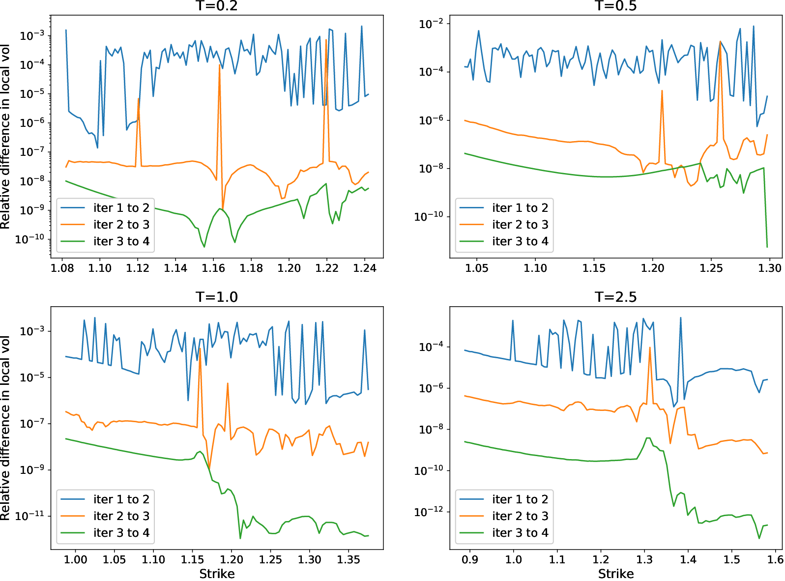
Figure 4.3: The local volatility update |σI+1LV−σILV|σILV\frac{|\sigma^{\text{LV}}_{I+1}-\sigma^{\text{LV}}_{I}|}{\sigma^{\text{LV}}_{I}} after iterations I=1,2,3I=1,2,3, at several time slices

We simulate 1000 paths and their antithetic conjugate to compute the Monte Carlo average of [Dtj​(Ktjl​rtjd−Stj​rtjf)​𝟙Stj>Ktjl]\left[D_{t_{j}}(K^{l}_{t_{j}}r_{t_{j}}^{d}-S_{t_{j}}r_{t_{j}}^{f})\mathds{1}_{S_{t_{j}}>K^{l}_{t_{j}}}\right] for all KtjlK^{l}_{t_{j}} in the strike grid at time slice tjt_{j}, which we plug in to the expectation in (4.2) to compute σLV​(Ktjl,tj)\sigma^{\text{LV}}(K^{l}_{t_{j}},t_{j}). The number of iterations at each time slice is set to 4.

In Figure 4.1 the surface plot can be seen as a visual evidence that the local volatility calibration completed smoothly. To see the impact of successive iterations, we plot the local volatility curve after each iteration at time slices tj=0.2,0.5,1.0,2.5t_{j}=0.2,0.5,1.0,2.5 in Figure 4.2. As can be seen in the plots, the successive iterations do not result in a visual change in the calibrated local volatility values. In Figure 4.3 we see that the relative differences in local volatility between successive iterations shrinks fast, which shows that the impact of each additional iteration is relatively low. As the computational time scales linearly with the number of iterations, we conclude that convergence is achieved by as low as a single iteration.

Refer to caption
Figure 4.4: Comparing Monte Carlo prices to market prices of vanilla call options at several time slices. The differences are within two Monte Carlo error bounds.

Finally, to validate the quality of the calibrated volatility surface, we run a successive simulation of (4.3), with the same setup we used for calibration, to price a range of vanilla call options with expiries T=0.2,0.5,1.0,2.5T=0.2,0.5,1.0,2.5. Figure 4.4 shows that the Monte Carlo prices match well with the market prices computed from the input implied volatility surface. The differences seem to be within two Monte Carlo errors.

5 Discussion

We derived the extension of the Dupire formula where the drift of the local volatility model is given as a difference of two stochastic processes of general form. The extended formula (2.18) can be used to calibrate local volatility models with stochastic rates of this structure. We further studied a general local volatility model where drift and diffusion are functions of arbitrary number of stochastic factors, with the simple assumption that the discount factor and the asset volatility are adapted functions of the Itô processes in the SDE system. The resulting generalized Dupire formula (3.6) can be used to calibrate a range of models, including stochastic local volatility models with stochastic interest rates. Both of these equations are given in implicit form, where the expectations on the right hand side depend on the local volatility (leverage) function. Such equations can be solved numerically by fixed-point iteration schemes. The expectations appearing in these equations have no known analytical solutions, yet they can be evaluated by numerical methods such as Monte Carlo or finite differences. We presented a case study to demonstrate a calibration scheme by Monte Carlo simulation. In the study we iteratively calibrated a local volatility model subject to stochastic dometic and foreign interest rates, which were chosen to follow an LGM process. The results show that the calibration is achieved after a single iteration by a relatively low number of simulation paths, and that the calibrated local volatility surface recovers market prices accurately.

Appendix A Total implied variance surface formulation

Quotes for various European call options with a range of strikes and maturities are required for the evaluation of the Dupire formula (2.21) or the extended Dupire formula (2.18) to create a local volatility surface. In practice, one can create a call price surface interpolator to evaluate the call price and its derivatives in these equations along the grid where the local volatility surface is being constructed. However the method for interpolation while evaluating the Dupire formula is a concern as the interpolated values might introduce arbitrage to the model. One way to address this problem is to construct a Black-Scholes total implied variance surface and interpolate that instead. As a matter of fact, practitioners typically work with market data that is in the form of parametrized or dense implied volatility surfaces that are calibrated with such penalty functions that aim to avoid or at least to minimize arbitrage. The absence of calendar spread arbitrage implies that the total implied variance surface is a monotonically increasing function of time [18, 19]. By construction, interpolating the total implied variance surface and using these values in the Dupire formula avoids calendar spread arbitrage. In this section we derive the total implied variance parametrization of the extended Dupire formula.

The Black-Scholes European call option price function CBSC_{\text{BS}} can be parametrized in terms of log-moneyness

y⁡(K,T)=log⁡KFT,y(K,T)=\log\frac{K}{F_{T}},

where FT≡S0​Pf​(0,T)Pd​(0,T)F_{T}\equiv S_{0}\frac{P^{f}(0,T)}{P^{d}(0,T)} is the forward price at time TT, and the total implied variance

w⁡(y⁡(K,T),T)=Σ​(K,T)2​Tw(y(K,T),T)=\Sigma(K,T)^{2}T

as [20]

CBS​(Pd​(0,T)​FT,y,w)=Pd​(0,T)​FT​(N⁡(d1)−ey​N​(d2))C_{\text{BS}}(P^{d}(0,T)F_{T},y,w)=P^{d}(0,T)F_{T}\left(N(d_{1})-e^{y}N(d_{2})\right) (A.1)

with

d1=−y​w−12+12​w12,d2=d1−w12.\begin{split}d_{1}=&-yw^{-\frac{1}{2}}+\frac{1}{2}w^{\frac{1}{2}},\\ d_{2}=&d_{1}-w^{\frac{1}{2}}.\end{split}

Here Σ⁡(K,T)\Sigma(K,T) is the market implied volatility at strike KK and maturity TT, and N⁡(⋅)N(\cdot) is the standard Gaussian cumulative distribution function. Noting that both CBSC_{\text{BS}} and ww depend on the strike KK indirectly through y⁡(K,T)y(K,T), that is CBS=CBS​(Pd​(0,T)​FT,y⁡(K,T),w⁡(y⁡(K,T),T))C_{\text{BS}}=C_{\text{BS}}(P^{d}(0,T)F_{T},y(K,T),w(y(K,T),T)), the first two derivatives of the call price with respect to the strike can be computed as

∂CBS∂K=(∂CBS∂y+∂CBS∂w​∂w∂y)​∂y∂K,∂2CBS∂K2=[∂2CBS∂y2+(2​∂2CBS∂w​∂y+∂2CBS∂w2​∂w∂y)​∂w∂y+∂CBS∂w​∂2w∂y2]​(∂y∂K)2+(∂CBS∂y+∂CBS∂w​∂w∂y)​∂2y∂K2.\begin{split}\frac{\partial C_{\text{BS}}}{\partial K}=&\left(\frac{\partial C_{\text{BS}}}{\partial y}+\frac{\partial C_{\text{BS}}}{\partial w}\frac{\partial w}{\partial y}\right)\frac{\partial y}{\partial K},\\ \frac{\partial^{2}C_{\text{BS}}}{\partial K^{2}}=&\left[\frac{\partial^{2}C_{\text{BS}}}{\partial y^{2}}+\left(2\frac{\partial^{2}C_{\text{BS}}}{\partial w\partial y}+\frac{\partial^{2}C_{\text{BS}}}{\partial w^{2}}\frac{\partial w}{\partial y}\right)\frac{\partial w}{\partial y}+\frac{\partial C_{\text{BS}}}{\partial w}\frac{\partial^{2}w}{\partial y^{2}}\right]\left(\frac{\partial y}{\partial K}\right)^{2}\\ &+\left(\frac{\partial C_{\text{BS}}}{\partial y}+\frac{\partial C_{\text{BS}}}{\partial w}\frac{\partial w}{\partial y}\right)\frac{\partial^{2}y}{\partial K^{2}}.\end{split}

Since ∂y∂K=1K\frac{\partial y}{\partial K}=\frac{1}{K} and ∂2y∂K2=−1K2\frac{\partial^{2}y}{\partial K^{2}}=-\frac{1}{K^{2}} the second expression can be written as

K2​∂2CBS∂K2=∂2CBS∂y2+(2​∂2CBS∂w​∂y+∂2CBS∂w2​∂w∂y−∂CBS∂w)​∂w∂y+∂CBS∂w​∂2w∂y2−∂CBS∂y.K^{2}\frac{\partial^{2}C_{\text{BS}}}{\partial K^{2}}=\frac{\partial^{2}C_{\text{BS}}}{\partial y^{2}}+\left(2\frac{\partial^{2}C_{\text{BS}}}{\partial w\partial y}+\frac{\partial^{2}C_{\text{BS}}}{\partial w^{2}}\frac{\partial w}{\partial y}-\frac{\partial C_{\text{BS}}}{\partial w}\right)\frac{\partial w}{\partial y}+\frac{\partial C_{\text{BS}}}{\partial w}\frac{\partial^{2}w}{\partial y^{2}}-\frac{\partial C_{\text{BS}}}{\partial y}. (A.2)

The right hand side of this equation demands evaluation of the derivatives of the call price with respect to the log-moneyness and the total implied variance. Using the identity N′​(d1)=ey​N′​(d2)N^{\prime}(d_{1})=e^{y}N^{\prime}(d_{2}) we compute the first ww-derivative as

∂CBS∂w=Pd​(0,T)​FT​[N′​(d1)​∂d1∂w−ey​N′​(d2)​∂d2∂w]=12​Pd​(0,T)​FT​ey​N′​(d2)​w−12;\displaystyle\begin{split}\frac{\partial C_{\text{BS}}}{\partial w}=&P^{d}(0,T)F_{T}\left[N^{\prime}(d_{1})\frac{\partial d_{1}}{\partial w}-e^{y}N^{\prime}(d_{2})\frac{\partial d_{2}}{\partial w}\right]\\ =&\frac{1}{2}P^{d}(0,T)F_{T}e^{y}N^{\prime}(d_{2})w^{-\frac{1}{2}};\end{split} (A.3)
and, since N′′​(x)=−x​N′​(x)N^{\prime\prime}(x)=-xN^{\prime}(x), the second ww-derivative evaluates as
∂2CBS∂w2=12​Pd​(0,T)​FT​ey​[−N′​(d2)​d2​∂d2∂w​w−12−12​N′​(d2)​w−32]=12​∂CBS∂w​[−14−1w+y2w2].\displaystyle\begin{split}\frac{\partial^{2}C_{\text{BS}}}{\partial w^{2}}=&\frac{1}{2}P^{d}(0,T)F_{T}e^{y}\left[-N^{\prime}(d_{2})d_{2}\frac{\partial d_{2}}{\partial w}w^{-\frac{1}{2}}-\frac{1}{2}N^{\prime}(d_{2})w^{-\frac{3}{2}}\right]\\ =&\frac{1}{2}\frac{\partial C_{\text{BS}}}{\partial w}\left[-\frac{1}{4}-\frac{1}{w}+\frac{y^{2}}{w^{2}}\right].\end{split} (A.4)
Furthermore, the remaining derivatives are
∂2CBS∂w​∂y=12​Pd​(0,T)​FT​ey​N′​(d2)​w−12​[−d2​∂d2∂y+1]=∂CBS∂w​[−yw+12],\displaystyle\begin{split}\frac{\partial^{2}C_{\text{BS}}}{\partial w\partial y}=&\frac{1}{2}P^{d}(0,T)F_{T}e^{y}N^{\prime}(d_{2})w^{-\frac{1}{2}}\left[-d_{2}\frac{\partial d_{2}}{\partial y}+1\right]\\ =&\frac{\partial C_{\text{BS}}}{\partial w}\left[-\frac{y}{w}+\frac{1}{2}\right],\end{split} (A.5)
∂CBS∂y=Pd​(0,T)​FT​[N′​(d1)​∂d1∂y−ey​N​(d2)−ey​N′​(d2)​∂d2∂y]=−Pd​(0,T)​FT​ey​N​(d2),\displaystyle\begin{split}\frac{\partial C_{\text{BS}}}{\partial y}=&P^{d}(0,T)F_{T}\left[N^{\prime}(d_{1})\frac{\partial d_{1}}{\partial y}-e^{y}N(d_{2})-e^{y}N^{\prime}(d_{2})\frac{\partial d_{2}}{\partial y}\right]\\ =&-P^{d}(0,T)F_{T}e^{y}N(d_{2}),\end{split} (A.6)
∂2CBS∂y2=−Pd​(0,T)​FT​ey​[N⁡(d2)+N′​(d2)​∂d2∂y]=∂CBS∂y+2​∂CBS∂w.\displaystyle\begin{split}\frac{\partial^{2}C_{\text{BS}}}{\partial y^{2}}=&-P^{d}(0,T)F_{T}e^{y}\left[N(d_{2})+N^{\prime}(d_{2})\frac{\partial d_{2}}{\partial y}\right]\\ =&\frac{\partial C_{\text{BS}}}{\partial y}+2\frac{\partial C_{\text{BS}}}{\partial w}.\end{split} (A.7)

Plugging in equations (A.3), (A.4), (A.5), (A.6), and (A.7) into (A.2) we arrive at

12​K2​∂2CBS∂K2=∂CBS∂w​[1−yw​∂w∂y+12​∂2w∂y2+14​(∂w∂y)2​(−14−1w+y2w2)].\frac{1}{2}K^{2}\frac{\partial^{2}C_{\text{BS}}}{\partial K^{2}}=\frac{\partial C_{\text{BS}}}{\partial w}\left[1-\frac{y}{w}\frac{\partial w}{\partial y}+\frac{1}{2}\frac{\partial^{2}w}{\partial y^{2}}+\frac{1}{4}\left(\frac{\partial w}{\partial y}\right)^{2}\left(-\frac{1}{4}-\frac{1}{w}+\frac{y^{2}}{w^{2}}\right)\right]. (A.8)

Finally, we use the identities

∂y∂T=−S0FT​∂Pf​(0,T)Pd​(0,T)∂T=ff​(0,T)−fd​(0,T),∂(Pd​(0,T)​FT)∂T=S0​∂(Pf​(0,T))∂T=−ff​(0,T)​Pd​(0,T)​FT,\begin{split}\frac{\partial y}{\partial T}=&-\frac{S_{0}}{F_{T}}\frac{\partial\frac{P^{f}(0,T)}{P^{d}(0,T)}}{\partial T}=f^{f}(0,T)-f^{d}(0,T),\\ \frac{\partial(P^{d}(0,T)F_{T})}{\partial T}=&S_{0}\frac{\partial(P^{f}(0,T))}{\partial T}=-f^{f}(0,T)P^{d}(0,T)F_{T},\end{split}

to formulate the time derivative of the call price as

∂CBS∂T=−ff​(0,T)​CBS+∂CBS∂w​∂w∂T+(∂CBS∂y+∂CBS∂w​∂w∂y)​(ff​(0,T)−fd​(0,T)).\frac{\partial C_{\text{BS}}}{\partial T}=-f^{f}(0,T)C_{\text{BS}}+\frac{\partial C_{\text{BS}}}{\partial w}\frac{\partial w}{\partial T}+\left(\frac{\partial C_{\text{BS}}}{\partial y}+\frac{\partial C_{\text{BS}}}{\partial w}\frac{\partial w}{\partial y}\right)(f^{f}(0,T)-f^{d}(0,T)). (A.9)

Plugging in equations (A.8) and (A.9) into (2.18) gives us the extended Dupire formula in the log-moneyness/total implied variance parametrization.

σLV​(K,T)2=∂CBS∂T−Pd​(0,T)​𝐄ℚT​[(K​rTd−ST​rTf)​𝟙ST>K]∂CBS∂w​[1−yw​∂w∂y+12​∂2w∂y2+14​(∂w∂y)2​(−14−1w+y2w2)],\sigma^{\text{LV}}(K,T)^{2}=\frac{\frac{\partial C_{\text{BS}}}{\partial T}-P^{d}(0,T)\mathbf{E}^{\mathbb{Q}^{\text{T}}}\left[(Kr_{T}^{d}-S_{T}r_{T}^{f})\mathds{1}_{S_{T}>K}\right]}{\frac{\partial C_{\text{BS}}}{\partial w}\left[1-\frac{y}{w}\frac{\partial w}{\partial y}+\frac{1}{2}\frac{\partial^{2}w}{\partial y^{2}}+\frac{1}{4}\left(\frac{\partial w}{\partial y}\right)^{2}\left(-\frac{1}{4}-\frac{1}{w}+\frac{y^{2}}{w^{2}}\right)\right]}, (A.10)

where the explicit forms of CBSC_{\text{BS}}, ∂CBS∂w\frac{\partial C_{\text{BS}}}{\partial w}, ∂CBS∂y\frac{\partial C_{\text{BS}}}{\partial y}, and ∂CBS∂T\frac{\partial C_{\text{BS}}}{\partial T} are given by (A.1), (A.3), (A.6), and (A.9) respectively.

Equation (3.11) allows us to write the extended Dupire formula for the two stochastic rates and stochastic local volatility model (3.9) in the total implied variance surface formulation as well. Since the deterministic local volatility limiting case was already computed in this formulation as in (A.10), we can write the leverage function for the stochastic local volatility generalization as

Ls​(K,T)2=∂CBS∂T−Pd​(0,T)​𝐄ℚT​[(K​rTd−ST​rTf)​𝟙ST>K]∂CBS∂w​[1−yw​∂w∂y+12​∂2w∂y2+14​(∂w∂y)2​(−14−1w+y2w2)]​𝐄ℚT​[UT|ST=K].L_{s}(K,T)^{2}=\frac{\frac{\partial C_{\text{BS}}}{\partial T}-P^{d}(0,T)\mathbf{E}^{\mathbb{Q}^{\text{T}}}\left[(Kr_{T}^{d}-S_{T}r_{T}^{f})\mathds{1}_{S_{T}>K}\right]}{\frac{\partial C_{\text{BS}}}{\partial w}\left[1-\frac{y}{w}\frac{\partial w}{\partial y}+\frac{1}{2}\frac{\partial^{2}w}{\partial y^{2}}+\frac{1}{4}\left(\frac{\partial w}{\partial y}\right)^{2}\left(-\frac{1}{4}-\frac{1}{w}+\frac{y^{2}}{w^{2}}\right)\right]\mathbf{E}^{\mathbb{Q}^{\text{T}}}\left[U_{T}|S_{T}=K\right]}.
Single stochastic rate limit

In the limit where the foreign rates rTfr_{T}^{f} are deterministic, this equation becomes

σLV​(K,T)2=∂CBS∂w​∂w∂T−fd​(0,T)​(∂CBS∂y+∂CBS∂w​∂w∂y)−Pd​(0,T)​K​𝐄ℚT​[rTd​𝟙ST>K]∂CBS∂w​[1−yw​∂w∂y+12​∂2w∂y2+14​(∂w∂y)2​(−14−1w+y2w2)].\sigma^{\text{LV}}(K,T)^{2}=\frac{\frac{\partial C_{\text{BS}}}{\partial w}\frac{\partial w}{\partial T}-f^{d}(0,T)\left(\frac{\partial C_{\text{BS}}}{\partial y}+\frac{\partial C_{\text{BS}}}{\partial w}\frac{\partial w}{\partial y}\right)-P^{d}(0,T)K\mathbf{E}^{\mathbb{Q}^{\text{T}}}\left[r_{T}^{d}\mathds{1}_{S_{T}>K}\right]}{\frac{\partial C_{\text{BS}}}{\partial w}\left[1-\frac{y}{w}\frac{\partial w}{\partial y}+\frac{1}{2}\frac{\partial^{2}w}{\partial y^{2}}+\frac{1}{4}\left(\frac{\partial w}{\partial y}\right)^{2}\left(-\frac{1}{4}-\frac{1}{w}+\frac{y^{2}}{w^{2}}\right)\right]}. (A.11)
Deterministic rates limit

In the limit where both the domestic rates rTdr_{T}^{d} and the foreign rates rTfr_{T}^{f} are deterministic, the equation further simplifies to the form given in [20]

σLV​(K,T)2=∂w∂T1−yw​∂w∂y+12​∂2w∂y2+14​(∂w∂y)2​(−14−1w+y2w2).\sigma^{\text{LV}}(K,T)^{2}=\frac{\frac{\partial w}{\partial T}}{1-\frac{y}{w}\frac{\partial w}{\partial y}+\frac{1}{2}\frac{\partial^{2}w}{\partial y^{2}}+\frac{1}{4}\left(\frac{\partial w}{\partial y}\right)^{2}\left(-\frac{1}{4}-\frac{1}{w}+\frac{y^{2}}{w^{2}}\right)}. (A.12)

Acknowledgments

The authors are grateful to the SIAM SIFIN reviewers and the editor for their valuable comments that have substantially improved the paper. The authors are indebted to Dooheon Lee for numerous enlightening discussions and guidance about the construction and the flow of this paper. The authors would also like to thank Agus Sudjianto for supporting this research, and Vijayan Nair for suggestions, feedback, and discussion regarding this work. Orcan Ogetbil is appreciative for Paul Feehan’s original introduction to the subject and his endorsement. Any opinions, findings and conclusions or recommendations expressed in this material are those of the author and do not necessarily reflect the views of Wells Fargo Bank, N.A., its parent company, affiliates and subsidiaries.

References

  • [1] Bruno Dupire. Pricing with a Smile. Risk Magazine, pages 18–20, 1 1994.
  • [2] Emanuel Derman and Iraj Kani. Riding on a Smile. Risk Magazine, pages 32–39, 2 1994.
  • [3] Leif Andersen and Jesper Andreasen. Jump-Diffusion Processes: Volatility Smile Fitting and Numerical Methods for Option Pricing. Review of Derivatives Research, 4(3):231–262, 2000.
  • [4] Eric Benhamou, Arnaud Rivoira, and Anne Gruz. Stochastic Interest Rates for Local Volatility Hybrids Models, 2008.
  • [5] Bing Hu. Local Volatility Model with Stochastic Interest Rate. Master’s thesis, York University, 8 2015.
  • [6] Michal Jex, R. C. W. Henderson, and Desheng Wang. Pricing Exotics Under the Smile. Risk Magazine, 12:72–75, 11 1999.
  • [7] Alexander Lipton. The vol smile problem. Risk Magazine, 15(2):61–66, 2 2002.
  • [8] Yu Tian, Zili Zhu, Geoffrey Lee, Fima Klebaner, and Kais Hamza. Calibrating and Pricing with a Stochastic-Local Volatility Model. The Journal of Derivatives, 22(3):21–39, 2015.
  • [9] Ben M. Hambly, Matthieu Mariapragassam, and Christoph Reisinger. A forward equation for barrier options under the Brunick & Shreve Markovian projection. Quantitative Finance, 16:827 – 838, 2014.
  • [10] Julien Guyon and Pierre Henry-Labordère. Being particular about calibration. Risk Magazine, 2012.
  • [11] Griselda Deelstra and Grégory Rayée. Local Volatility Pricing Models for Long-dated FX Derivatives. Applied Mathematical Finance, 20(1204.0633):380–402, 2013.
  • [12] W. Feller. On the Theory of Stochastic Processes, with Particular Reference to Applications. In Proceedings of the [First] Berkeley Symposium on Mathematical Statistics and Probability, pages 403–432, Berkeley, Calif., 1949. University of California Press.
  • [13] John C. Cox, Jonathan E. Ingersoll, and Stephen A. Ross. A Theory of the Term Structure of Interest Rates. Econometrica, 53(2):385–407, 1985.
  • [14] G. Tataru, T. Fisher, and J. Yiu. The Bloomberg Stochastic Local Volatility Model For FX Exotics. Bloomberg, 2012.
  • [15] István Gyöngy. Mimicking the one-dimensional marginal distributions of processes having an Ito differential. Probability Theory and Related Fields, 71:501–516, 1986.
  • [16] P. S. Hagan and Diana E. Woodward. Markov interest rate models. Applied Mathematical Finance, 6:233–260, 1999.
  • [17] Roland Lichters, Roland Stamm, and Donal Gallagher. Modern derivatives pricing and credit exposure analysis: theory and practice of CSA and XVA pricing, exposure simulation and backtesting. Springer, 2015.
  • [18] Matthias R. Fengler. Arbitrage-free smoothing of the implied volatility surface. Quantitative Finance, 9(4):417–428, 2009.
  • [19] Jim Gatheral and Antoine Jacquier. Arbitrage-free SVI volatility surfaces. Quantitative Finance, 14(1):59–71, 2014.
  • [20] Jim Gatheral. The Volatility Surface, chapter 1, pages 1–14. John Wiley & Sons, Ltd, 2012.