Stability-enhanced AP IMEX1-LDG method: energy-based stability and rigorous AP property

Zhichao Peng Thanks: Department of Mathematical Sciences, Rensselaer Polytechnic Institute, Troy, NY 12180, U.S.A. pengz2@rpi.edu Yingda Cheng Thanks: Department of Mathematics, Department of Computational Mathematics, Science and Engineering, Michigan State University, East Lansing, MI 48824 U.S.A. ycheng@msu.edu. Research is supported by NSF grants DMS-1453661 and DMS-1720023. Jing-Mei Qiu Thanks: Department of Mathematical Sciences, University of Delaware, Newark, DE, 19716, U.S.A. jingqiu@udel.edu. Research is supported by NSF grant DMS-1818924 and AFOSR grant FA9550-18-1-0257. Fengyan Li Thanks: Department of Mathematical Sciences, Rensselaer Polytechnic Institute, Troy, NY 12180, U.S.A. lif@rpi.edu. Research is supported by NSF grants DMS-1719942 and DMS-1913072.

Abstract

In our recent work [22], a family of high order asymptotic preserving (AP) methods, termed as IMEX-LDG methods, are designed to solve some linear kinetic transport equations, including the one-group transport equation in slab geometry and the telegraph equation, in a diffusive scaling. As the Knudsen number $\varepsilon$ goes to zero, the limiting schemes are implicit discretizations to the limiting diffusive equation. Both Fourier analysis and numerical experiments imply the methods are unconditionally stable in the diffusive regime when $\varepsilon\ll 1$ . In this paper, we develop an energy approach to establish the numerical stability of the IMEX1-LDG method, the sub-family of the methods that is first order accurate in time and arbitrary order in space, for the model with general material properties. Our analysis is the first to simultaneously confirm unconditional stability when $\varepsilon\ll 1$ and the uniform stability property with respect to $\varepsilon$ . To capture the unconditional stability, a novel discrete energy is introduced by better exploring the contribution of the scattering term in different regimes. A general form of the weight function, introduced to obtain the unconditional stability for $\varepsilon\ll 1$ , is also for the first time considered in such stability analysis. Based on the uniform stability, a rigorous asymptotic analysis is then carried out to show the AP property.

1 Introduction

In this paper, we continue our efforts in devising and advancing mathematical understanding of asymptotic preserving (AP) methods to solve time-dependent multi-scale kinetic transport equations within the discontinuous Galerkin (DG) framework [12, 11, 22]. Particularly, we focus on establishing energy-type numerical stability and the AP property for some methods proposed in [22] for the following model equation,

{\mathcal{P}}^{\varepsilon}:\qquad\varepsilon f_{t}+v\partial_{x}f=\frac{\sigma_{s}}{\varepsilon}\left(\langle f\rangle-f\right)-\varepsilon\sigma_{a}f,

(1.1)

with periodic boundary conditions. The function $f=f(x,v,t)$ is the probability distribution function of the particles, with the space variable $x\in\Omega_{x}\subset{\mathbb{R}}$ , velocity variable $v\in\Omega_{v}\subset{\mathbb{R}}$ , and time $t\geq 0$ . $\sigma_{s}(x)>0$ and $\sigma_{a}(x)\geq 0$ are the scattering and absorption coefficients, respectively. ${\mathcal{L}}(f)=\langle f\rangle-f$ defines a scattering operator, where $\langle f\rangle:=\int_{\Omega_{v}}fd\nu$ and $\nu$ is a measure of the velocity space satisfying $\int_{\Omega_{v}}1d\nu=1$ . The parameter $\varepsilon>0$ is the dimensionless Knudsen number, defined as the ratio of the mean free path of the particles over the characteristic length of the system. The model (1.1) is in a diffusive scaling, and as $\varepsilon\rightarrow 0$ , it approaches its diffusive limit

{\mathcal{P}}^{0}:\qquad\partial_{t}\rho=\langle v^{2}\rangle\partial_{x}(\partial_{x}\rho/\sigma_{s})-\sigma_{a}\rho.

(1.2)

Here $\rho=\langle f\rangle$ is the macroscopic density. Though seemingly simple, the equation in (1.1) provides a prototype model to study many realistic problems such as in neutron transport or radiative transfer theory both numerically and mathematically.

To simulate multi-scale models like that in (1.1) effectively and reliably for a broad range of value for $\varepsilon$ , AP methods are widely recognized by the scientific community (see e.g. review papers [13, 5]). These methods are designed for the governing model with $\varepsilon>0$ . Additionally when $\varepsilon\rightarrow 0$ , the methods become consistent and stable discretizations for the limiting model as in (1.2) even on under-resolved meshes with $\Delta x,\Delta t\gg\varepsilon$ . Hence, AP methods provide a natural transition of different regimes in multi-scale simulations. AP methods usually involve some level of implicit treatment to deal with the stiffness of the model when $\varepsilon\ll 1$ . It is known that stability alone does not guarantee the scheme to capture the correct asymptotic limit [3, 20].

In our recent work [22], a family of high order AP methods, termed as IMEX-LDG methods, are designed for (1.1). The methods are based on the reformulation of the equation, and involve local DG (LDG) discretization in space [4], globally stiffly accurate implicit-explicit (IMEX) Runge-Kutta (RK) methods in time [2], and a judicially chosen IMEX strategy. The reformulation has two steps: micro-macro decomposition [19, 17], and addition/subtraction of a $\omega$ -weighted diffusive term [2]. The latter is introduced to obtain fully implicit limiting schemes as $\varepsilon\rightarrow 0$ , to achieve unconditional stability of the methods in the diffusive regime with $\varepsilon\ll 1$ , hence to circumvent the otherwise stringent parabolic type time step condition in this regime, namely, $\Delta t=O(\Delta x^{2})$ , of many AP schemes whose limiting schemes are explicit [14, 15, 17, 12]. Using globally stiffly accurate IMEX RK methods in time, and LDG methods in space with suitable numerical fluxes, the IMEX-LDG methods project the numerical solutions to the local equilibrium at both inner stages and full RK steps in the limit of $\varepsilon\rightarrow 0$ , and this is important for the AP property and seemingly also for accuracy (see appendix of [22]). In [22], unconditional stability in the diffusive regime is observed numerically, and is confirmed by a Fourier-type stability analysis applied to the two-velocity telegraph equation with ${\Omega_{v}}=\{-1,+1\}$ , and constant material properties $\sigma_{s}=1$ , $\sigma_{a}=0$ .

In this work we restrict our attention to the IMEX1-LDG method, the sub-family of the methods in [22] that is first order accurate in time and arbitrary order in space, and examine it systematically for the model with the general material properties, namely with the spatially varying scattering and absorption coefficients $\sigma_{s}(x)$ and $\sigma_{a}(x)$ . Our main objectives are two-fold. The first is to establish unconditional stability in the diffusive regime with $\varepsilon\ll 1$ as well as uniform stability with respect to $\varepsilon$ . By following an energy approach as in [18, 11], one can get uniform stability yet fails to capture the unconditional stability for $\varepsilon\ll 1$ . Note the methods examined in [18, 11] in the limit of $\varepsilon\rightarrow 0$ are explicit. We instead propose and work with a new notion of $\mu$ -stability, and get the stability we want by better exploring the contribution of the scattering operator. The stability results up to this point depend on a parameter $\mu$ . An intricate algebraic-based optimization with respect to the admissible $\mu$ is subsequently followed, to further maximize the unconditional stability region, while also maximizing the allowable time step size in the regime when the method is conditionally stable. As our second objective, a rigorous asymptotic analysis is proved to show the AP property based on the uniform stability. To our best knowledge, our analysis is the first to capture unconditional stability when $\varepsilon\ll 1$ along with uniform stability property for the model (1.1) with general material properties. A general form of the weight function $\omega$ is also for the first time considered in such stability analysis. In this work, we keep the velocity variable continuous, and our analysis can be easily adapted when the velocity variable is further discretized such as by discrete ordinates or $P_{N}$ methods [23]. Our analysis can also be extended to AP methods with the same IMEX strategy yet with other spatial discretizations, as long as they satisfy some key properties, such as the adjoint property in (2.16) (also see Lemma 3.5 in [22]) and the stabilization as in (5.5) due to the upwind treatment. Though not presented here, a priori error estimates can follow similarly as in [11], and they are uniform in $\varepsilon$ for smooth enough solutions with uniform bounds in $\varepsilon$ under the relevant Sobolev norms. What seems to be more challenging and left to our future endeavor is to obtain the stability analysis for IMEX-LDG methods with higher order temporal accuracy.

Finally we want to briefly review some related literature especially in establishing numerical stability of AP methods for kinetic transport models in a diffusive scaling. One commonly used approach is Fourier type analysis. For the telegraph equation with ${\Omega_{v}}=\{-1,+1\}$ , an analytical time step condition is given in [17] via Fourier analysis to ensure uniform $L^{2}$ -stability of a first order finite difference AP method, while in [22], necessary conditions on $\varepsilon,\Delta x,\Delta t$ are obtained numerically for the $p$ -th order IMEX-LDG AP scheme ( $p=1,2,3$ ) to ensure an $L^{2}$ energy non-increasing in time. The results seem to be uniform in $\varepsilon$ , with unconditional stability captured for $\varepsilon\ll 1$ . Klar and Unterreiter in [16] considered a formally first-order in time and second-order in space AP scheme for the one-group transport equation with ${\Omega_{v}}=[-1,1]$ and established uniform stability by first establishing the result in Fourier space and then transforming it back to the physical space. Their analysis assumes the $H^{1}$ smoothness of the initial data. It is known that Fourier-type analysis requires uniform meshes and the models being linear and constant-coefficient. Energy-based stability analysis on the other hand does not pose these restrictions, yet they are not always easy to get. In [18], Liu and Mieussens revisited the first order AP method in [17] for a more general kinetic transport model and proved uniform stability following an energy approach. A similar analysis is carried out in [11] for the first order in time DG-IMEX1 method in [12]. Based on the uniform stability analysis, error estimates and rigorous asymptotic analysis are also established in [11]. In both [22] and here in this work, we want to capture the unconditional stability in the diffusive regime in addition to the uniform stability. Few other theoretical works, among many, for AP methods include uniform consistency [3, 15], uniform convergence [8, 7] based on the commuting diagram of AP schemes (see Fig 1.1 in [8]), and a recent work on uniform accuracy with IMEX multi-step methods [10].

The remaining of the paper is organized as follows. In Section 2, we review and extend the IMEX1-LDG method in [22] to our model (1.1) with general material properties. Section 3 presents main results on numerical stability. Here several theorems, including Theorem 3.1 and Theorem 3.3, are stated to obtain uniform stability, while capturing the unconditional stability in the diffusive regime. An optimization step is carried out in Theorem 3.4 to find the best value of the parameter $\mu$ in the notion of $\mu$ -stability in order to optimize the stability results. Once uniform stability is available, the AP property of the method is stated in Theorem 4.1 in Section 4. The proofs of all major theorems are presented in Sections 5-7 for better readability.

2 The IMEX1-LDG scheme

In this section, we will review the IMEX1-LDG method proposed in [22] and extend it more systematically to the model (1.1) with general material properties $\sigma_{s}(x)$ and $\sigma_{a}(x)$ , both being in $L^{\infty}(\Omega_{x})$ and satisfying $\sigma_{M}\geq\sigma_{s}(x)\geq\sigma_{m}>0,\sigma_{a}(x)\geq 0,\forall x\in{\Omega_{x}}$ . The boundary conditions in space are periodic, and the velocity variable $v$ will not be discretized.

Two examples of the model (1.1) will be examined. One is the one-group transport equation in slab geometry. Here $\Omega_{v}=[-1,1]$ and the measure $\nu$ is defined as $\int_{\Omega_{v}}fd\nu=\frac{1}{2}\int_{\Omega_{v}}f(x,v,t)dv,$ with $dv$ being the standard Lebesgue measure. The other is the telegraph equation with $\Omega_{v}=\{-1,1\}$ , and $\nu$ is a discrete measure, given as $\int_{\Omega_{v}}fd\nu=\frac{1}{2}\left(f(x,v=1,t)+f(x,v=-1,t)\right).$ There is little difference in the formulation and analysis of the IMEX1-LDG method for both examples.

2.1 Reformulation

The IMEX1-LDG method is defined based on a reformulation of (1.1), which is obtained in several steps. As the first step, we rewrite the model into its micro-macro decomposition [19, 17]. Let $L^{2}(\Omega_{v},\nu)$ be the square integrable space in $v$ , with the inner product $\langle f,g\rangle:=\langle fg\rangle$ . Let $\Pi$ be the $L^{2}$ projection onto $\textrm{Null}({\mathcal{L}})=\text{Span}\{1\}$ , $\mathbf{I}$ be the identify operator, and $\rho:=\langle f\rangle=\Pi f$ be the macroscopic density. Then $f$ can be decomposed orthogonally into $f=\rho+\varepsilon g$ , with $\rho$ and $g$ satisfying


		$\displaystyle\partial_{t}\rho+\partial_{x}\langle vg\rangle=-\sigma_{a}\rho,$		(2.1a)
		$\displaystyle\partial_{t}g+\frac{1}{\varepsilon}(\mathbf{I}-\Pi)(v\partial_{x}g)+\frac{1}{\varepsilon^{2}}v\partial_{x}\rho=-\frac{\sigma_{s}}{\varepsilon^{2}}g-\sigma_{a}g.$		(2.1b)

This is the micro-macro decomposition. As $\varepsilon\rightarrow 0$ , the equations (2.1) formally become

\partial_{t}\rho+\partial_{x}\langle vg\rangle=-\sigma_{a}\rho,\quad\sigma_{s}g=-v\partial_{x}\rho,

(2.2)

which is a first order form of the limiting diffusion equation,

\partial_{t}\rho=\langle v^{2}\rangle\partial_{x}\left(\partial_{x}\rho/\sigma_{s}\right)-\sigma_{a}\rho,

(2.3)

equipped with the compatible initial condition. The relation $\sigma_{s}g=-v\partial_{x}\rho$ in (2.2) will be referred to as the local equilibrium. For the telegraph equation, the diffusion constant is $\langle v^{2}\rangle=1$ , while for the one-group transport equation in slab geometry, $\langle v^{2}\rangle=1/3$ .

As the second step, a weighted diffusion term, $\omega\langle v^{2}\rangle\partial_{x}(\partial_{x}\rho/\sigma_{s})$ , is added to both sides of (2.1a), leading to


		$\displaystyle\partial_{t}\rho+\partial_{x}\langle vg\rangle+\omega\langle v^{2}\rangle\partial_{x}\left(\partial_{x}\rho/\sigma_{s}\right)=\omega\langle v^{2}\rangle\partial_{x}\left(\partial_{x}\rho/\sigma_{s}\right)-\sigma_{a}\rho,$		(2.4a)
		$\displaystyle\partial_{t}g+\frac{1}{\varepsilon}(\mathbf{I}-\Pi)(v\partial_{x}g)+\frac{1}{\varepsilon^{2}}v\partial_{x}\rho=-\frac{\sigma_{s}}{\varepsilon^{2}}g-\sigma_{a}g.$		(2.4b)

Here the weight function $\omega$ is non-negative and bounded. It is independent of $x$ and can depend on $\varepsilon$ , satisfying

\omega\rightarrow 1,\quad\text{as}\quad\varepsilon\rightarrow 0.

(2.5)

Additional properties desired for $\omega$ in general and considered specifically in this work will be discussed in next subsection. The idea of reformulating a kinetic transport model in the diffusive scaling based on adding and subtracting a diffusive term was previously used in [2] and [6] to remove some parabolic stiffness in designing AP schemes. One advancement we made in [22] and here is to improve the mathematical understanding of the desired property and the role of the weight function $\omega$ , and such advancement can guide one to choose $\omega$ in practice.

With the auxiliary variables $q=\partial_{x}\rho$ and $u=q/\sigma_{s}$ , the system (2.4) can also be written in its first order form


		$\displaystyle q=\partial_{x}\rho,\qquad u=q/\sigma_{s},$		(2.6a)
		$\displaystyle\partial_{t}\rho+\partial_{x}\langle v(g+\omega vu)\rangle=\omega\langle v^{2}\rangle\partial_{x}u-\sigma_{a}\rho,$		(2.6b)
		$\displaystyle\partial_{t}g+\frac{1}{\varepsilon}(\mathbf{I}-\Pi)(v\partial_{x}g)+\frac{1}{\varepsilon^{2}}v\partial_{x}\rho=-\frac{\sigma_{s}}{\varepsilon^{2}}g-\sigma_{a}g,$		(2.6c)

and correspondingly its limiting system as $\varepsilon\rightarrow 0$ now is

\partial_{t}\rho=\langle v^{2}\rangle\partial_{x}u-\sigma_{a}\rho,\quad q=\partial_{x}\rho=\sigma_{s}u,\quad g=-vq/\sigma_{s}=-vu.

(2.7)

The property (2.5) has been used. The introduction of $u$ is to deal with the spatially varying scattering coefficient $\sigma_{s}$ . Note that the term $v\partial_{x}\rho$ in (2.6c) can be replaced by $vq$ .

2.2 The IMEX1-LDG scheme

To present the scheme, we start with some notation. For the computational domain $\Omega_{x}=[x_{L},x_{R}]$ in space, a mesh, $x_{L}=x_{\frac{1}{2}}<x_{\frac{3}{2}}<\dots<x_{N+\frac{1}{2}}=x_{R}$ , is introduced. Let $I_{i}=[{x_{i-\frac{1}{2}}},{x_{i+\frac{1}{2}}}]$ be an element, with $x_{i}$ as its center and $h_{i}$ as its length. Set $h=\max_{i}h_{i}$ . ( $\Delta x$ in the introduction is just $h$ here.) For any nonnegative integer $k$ , we define a finite dimensional discrete space

U_{h}^{k}=\left\{u\in L^{2}(\Omega_{x}):u|_{I_{i}}\in P^{k}(I_{i}),\forall i\right\},

(2.8)

where the local space $P^{k}(I)$ consists of polynomials of degree at most $k$ on $I$ . We also introduce

G_{h}^{k}=\left\{u(\cdot,v)\in U_{h}^{k}:\;\;\int_{\Omega_{v}}\int_{\Omega_{x}}|u(x,v)|^{2}dxdv<\infty\right\}.

(2.9)

For a function $\phi\in U_{h}^{k}$ , we write $\phi(x^{\pm})=\lim_{\Delta x\rightarrow 0^{\pm}}\phi(x+\Delta x)$ , and $\phi^{\pm}_{i+\frac{1}{2}}=\phi(x^{\pm}_{i+\frac{1}{2}})$ . The jump and average of $\phi$ at $x_{i+\frac{1}{2}}$ are defined as $[\phi]_{i+\frac{1}{2}}={\phi_{i+\frac{1}{2}}^{+}-\phi_{i+\frac{1}{2}}^{-}}$ and $\{\phi\}_{i+\frac{1}{2}}=\frac{1}{2}(\phi_{i+\frac{1}{2}}^{+}+\phi_{i+\frac{1}{2}}^{-})$ , respectively.

The IMEX1-LDG scheme in [22] involves a LDG discretization in space and a first order globally stiffly accurate IMEX RK scheme in time. And an IMEX strategy is adopted so that all the terms, which are formally dominating in the regime $\varepsilon\ll 1$ , are treated implicitly. The IMEX1-LDG scheme for the model with a general $\sigma_{s}$ is based on the system (2.6), and it is defined as below. Given $\rho_{h}^{n},\;q_{h}^{n},\;u_{h}^{n}\in U_{h}^{k}$ , $g_{h}^{n}\in G_{h}^{k}$ that approximate the solution $\rho$ , $q=\partial_{x}\rho$ , $u$ , and $g$ at $t^{n}$ , we look for $\rho_{h}^{n+1},\;q_{h}^{n+1},\;u_{h}^{n+1}\in U_{h}^{k}$ , $g_{h}^{n+1}\in G_{h}^{k}$ at $t^{n+1}=t^{n}+\Delta t$ , such that $\forall\;{\varphi},{\eta},{\phi}\in U_{h}^{k}$ and ${\psi}\in G_{h}^{k}$ ,


		$\displaystyle(q_{h}^{n+1},{\varphi})+d_{h}(\rho_{h}^{n+1},{\varphi})=0,$		(2.10a)
		$\displaystyle(\sigma_{s}u_{h}^{n+1},{\eta})=(q_{h}^{n+1},{\eta}),$		(2.10b)
		$\displaystyle\big(\frac{\rho_{h}^{n+1}-\rho_{h}^{n}}{\Delta t},{\phi}\big)+l_{h}(\langle v(g_{h}^{n}+\omega vu_{h}^{n})\rangle,{\phi})=\omega\langle v^{2}\rangle l_{h}(u_{h}^{n+1},{\phi})-\left(\sigma_{a}\rho_{h}^{n+1},{\phi}\right),$		(2.10c)
		$\displaystyle\big(\frac{g_{h}^{n+1}-g_{h}^{n}}{\Delta t},{\psi}\big)+\frac{1}{\varepsilon}b_{h,v}(g_{h}^{n},{\psi})-\frac{v}{\varepsilon^{2}}d_{h}(\rho_{h}^{n+1},{\psi})=-\frac{1}{\varepsilon^{2}}(\sigma_{s}g_{h}^{n+1},{\psi})-\left(\sigma_{a}g_{h}^{n+1},{\psi}\right).$		(2.10d)

Here $(\cdot,\cdot)$ is the standard inner product for $L^{2}(\Omega_{x})$ . The bilinear forms $d_{h},l_{h}$ , and $b_{h,v}$ are all related to discrete spatial derivatives, and defined as


$\displaystyle d_{h}(\rho_{h},{\varphi})$	$\displaystyle=\sum_{i}\int_{I_{i}}\rho_{h}\partial_{x}{\varphi}dx+\sum_{i}\breve{\rho}_{h,{i-\frac{1}{2}}}[{\varphi}]_{i-\frac{1}{2}},$	(2.11a)
$\displaystyle l_{h}(u_{h},{\phi})$	$\displaystyle=-\sum_{i}\int_{I_{i}}u_{h}\partial_{x}{\phi}dx-\sum_{i}\hat{u}_{h,{i-\frac{1}{2}}}[{\phi}]_{i-\frac{1}{2}},$	(2.11b)
$\displaystyle b_{h,v}(g_{h},{\psi})$	$\displaystyle=(({\bf{I}}-\Pi){\mathcal{D}}_{h}(g_{h};v),{\psi})=({\mathcal{D}}_{h}(g_{h};v)-\langle{\mathcal{D}}_{h}(g_{h};v)\rangle,{\psi}).$	(2.11c)

For a given $v\in\Omega_{v}$ , the function ${\mathcal{D}}_{h}(g_{h};v)\in U_{h}^{k}$ in (2.11c) is an upwind DG discretization of the transport term $v\partial_{x}g$ . It is determined by

\displaystyle({\mathcal{D}}_{h}(g_{h};v),{\psi})=-\sum_{i}\left(\int_{I_{i}}vg_{h}\partial_{x}{\psi}dx\right)-\sum_{i}\widetilde{(vg_{h})}_{i-\frac{1}{2}}[{\psi}]_{i-\frac{1}{2}},\quad\forall\psi\in U_{h}^{k},

(2.12)

where $\widetilde{vg}$ is the upwind flux,

\widetilde{vg}:=\left\{\begin{array}[]{ll}vg^{-},&\mbox{if}\;v>0\\ vg^{+},&\mbox{if}\;v<0\end{array}\right.=v\{g\}-\frac{|v|}{2}[g].

(2.13)

The terms $\breve{\rho}$ and $\hat{u}$ in (2.11a)-(2.11b) are one of the following alternating flux pair,

\textrm{right-left: }\;\;\;\;\breve{\rho}={\rho}^{+},\;\;\hat{u}=u^{-};\qquad\textrm{left-right: }\;\;\;\;\breve{\rho}={\rho}^{-},\;\;\hat{u}={u}^{+}.

(2.14)

The choice of the numerical fluxes $\breve{\rho}$ and $\hat{u}$ is important for the numerical solution to stay close to the local equilibrium when $\varepsilon\ll 1$ , and it contributes to the AP property of the scheme. Similar as in standard LDG methods, the auxiliary unknowns $q_{h}$ and $u_{h}$ can be locally represented hence eliminated in terms of $\rho_{h}$ .

At $t=0$ , the initialization is done via the $L^{2}$ projection $\pi_{h}$ onto $U_{h}^{k}$ , namely,

\rho_{h}^{0}(\cdot)=\pi_{h}\rho(\cdot,0),\quad g_{h}^{0}(\cdot,v)=\pi_{h}g(\cdot,v,0),\quad u_{h}^{0}(\cdot,v)=\pi_{h}(\sigma_{s}^{-1}\partial_{x}\rho).

(2.15)

To complete the formulation of the scheme, one needs to specify the weight function $\omega$ . In our previous work [22], Fourier-type stability analysis suggests that $\omega$ should be chosen in the form of $\omega=\omega(\frac{\varepsilon}{h},\frac{\varepsilon^{2}}{\Delta t})$ , to preserve the intrinsic scale of the underlying model. In this paper, we only consider $\omega=\omega(\varepsilon/(\sigma_{m}h))$ , which is independent of $\varepsilon^{2}/\Delta t$ . Some specific examples include $\omega=\exp\big({-\varepsilon}/({\sigma_{m}h})\big)$ and $\omega\equiv 1$ . One can also use a piecewise constant choice $\omega={\bf 1}_{\{\varepsilon/(\sigma_{m}h)\leq\alpha\}}$ , with some fixed positive constant $\alpha$ , see Remark 3.7 for a specific choice of $\alpha$ recommended by our stability analysis. (Here ${\bf 1}_{D}$ is an indicator function with respect to a set $D$ .) Note that all these choices are non-negative and independent of $x$ , satisfying (2.5).

The next lemma states the relation of bilinear forms $d_{h}$ and $l_{h}$ , and this can be verified directly.

Lemma 2.1.

With either alternating flux pair in (2.14), the bilinear forms $b_{h}$ and $l_{h}$ are related,

\displaystyle l_{h}({\varphi},{\phi})=d_{h}({\phi},{\varphi}),\qquad\forall\varphi,\;\phi\in U_{h}^{k}.

(2.16)

The unique solvability of the solution to the IMEX1-LDG method is given in next proposition, together with some properties in (2.17) that can be easily verified. The key to prove the first part of the proposition is the unique solvability of the problem examined in Lemma 2.3.

Proposition 2.2.

The IMEX1-LDG method is uniquely solvable for any $\varepsilon\geq 0$ . In addition, the solution satisfies

\langle g_{h}^{n}\rangle=0,\;\forall n\geq 0,\qquad(\sigma_{s}u_{h}^{m},{\eta})=-l_{h}({\eta},\rho_{h}^{m}),\;\forall{\eta}\in U_{h}^{k},\;\;\forall m\geq 1.

(2.17)

Lemma 2.3.

Given $S\in L^{2}(\Omega_{x})$ and $\gamma_{j}\geq 0,j=1,2$ . Consider the following problem: look for $\rho_{h},q_{h},u_{h}\in U_{h}^{k}$ , such that $\forall{\varphi},{\eta},{\phi}\in U_{h}^{k}$ ,

(q_{h},{\varphi})+d_{h}(\rho_{h},{\varphi})=0,\quad(\sigma_{s}u_{h},{\eta})=(q_{h},{\eta}),\quad(\rho_{h},{\phi})-\gamma_{1}l_{h}(u_{h},{\phi})=-\gamma_{2}(\sigma_{a}\rho_{h},{\phi})+(S,{\phi}).

(2.18)

Then $\rho_{h},q_{h},u_{h}$ are uniquely solvable.

Proof.

We first consider the homogeneous case with $S=0$ . Take ${\varphi}={\eta}=u_{h},{\phi}=\rho_{h}$ , use the relation of $d_{h}$ and $l_{h}$ , we get

(\rho_{h},\rho_{h})+\gamma_{1}(\sigma_{s}u_{h},u_{h})+\gamma_{2}(\sigma_{a}\rho_{h},\rho_{h})=0.

With $\gamma_{1},\gamma_{2},\sigma_{s},\sigma_{a}$ being non-negative, one has $\rho_{h}=0$ , and the equations in (2.18) further ensure $q_{h}=u_{h}=0$ . This, in combination with the linearity of the problem as well as that both the solution and the test function are from the same finite dimensional space $U_{h}^{k}$ , implies the unique solvability of the problem with the general source term $S$ . ∎

Following the formal asymptotic analysis as in [22], we can show the IMEX1-LDG method is AP, namely as $\varepsilon\rightarrow 0$ , its limiting scheme is a consistent and stable discretization of the limiting system (2.7), when the initial data is well-prepared. This will be stated in Section 4 and proved in Section 7 once the uniform stability is available. When the initial data is not well-prepared, our scheme can adopt a similar initial fix [22] when $n=0$ to stay AP. There is no change to numerical stability, while the AP property can be established rigorously and the details are not presented in this paper.

2.3 Norms, inverse inequalities, and more notation

We introduce some standard norms $||\phi||=||\phi||_{L^{2}({\Omega_{x}})}$ , $|||\phi|||=(\langle||\phi||^{2}\rangle)^{1/2}$ , and weighted norms $||\phi||_{s}=||\sqrt{\sigma_{s}}\phi||$ , $|||\phi|||_{s}=|||\sqrt{\sigma_{s}}\phi|||.$ For a bounded function $\psi(v)$ of $v$ , without confusion we will write $||\psi||_{\infty}=||\psi||_{L^{\infty}({\Omega_{v}})}$ . Even though for our specific examples with ${\Omega_{v}}=[-1,1]$ or $\{-1,1\}$ , we have $||v||_{\infty}=||v^{2}||_{\infty}=1$ , we still keep $||v||_{\infty}$ and $||v^{2}||_{\infty}$ in most results, to possibly inform about the case with a more general bounded velocity space ${\Omega_{v}}$ .

In our analysis, the following inverse inequalities will be frequently used, and they are fairly standard in finite element analysis: there exist constants $C_{inv}=C_{inv}(k)$ and $\widehat{C}_{inv}=\widehat{C}_{inv}(k)$ , such that for any $\phi\in P^{k}([a,b])$ ,


		$\displaystyle\|\phi(y)\|^{2}(b-a)\leq C_{inv}\int_{a}^{b}\|\phi(x)\|^{2}dx,\qquad\mbox{with}\;y=a\;\mbox{or}\;b,$		(2.19a)
		$\displaystyle(b-a)^{2}\int_{a}^{b}\|\phi^{\prime}(x)\|^{2}dx\leq\widehat{C}_{inv}\int_{a}^{b}\|\phi(x)\|^{2}dx.$		(2.19b)

Particularly, $C_{inv}(k)|_{k=0}=1$ . Next lemma states a property of the inverse constants $\widehat{C}_{inv},C_{inv}$ .

Lemma 2.4.

With $\Omega_{v}=[-1,1]$ or $\Omega_{v}=\{-1,1\}$ , and with $\widehat{C}_{inv}$ , $C_{inv}$ from (2.19), we define

{\mathcal{K}}={\mathcal{K}}(k)=\frac{8(C_{inv}||v||_{\infty})^{2}}{\widehat{C}_{inv}||v^{2}||_{\infty}}=\frac{8(C_{inv})^{2}}{\widehat{C}_{inv}}.

(2.20)

Then at least for $k=1,2,\cdots,9$ , we have ${\mathcal{K}}>1.$

Proof.

Based on Lemmas 1-2 in [24] and a linear scaling, one can take $C_{inv}=(k+1)^{2}$ and $\widehat{C}_{inv}=12k^{4}$ , which can be used to verify ${\mathcal{K}}>1$ directly for $k=1,2,\cdots 9$ . ∎

Sharper values of $C_{inv}(k)$ and $\widehat{C}_{inv}(k)$ can be numerically obtained for each $k$ by solving an eigenvalue problem (see Section 4.1 in [24]), hence one can check numerically whether ${\mathcal{K}}>1$ holds or not for larger $k$ . Given the temporal accuracy of the IMEX1-LDG method is first order, it is more than enough for us to consider $k\leq 9$ in our analysis.

For convenient reference, we summarize in Table 2.1 the definitions of some notation arising from analysis, including $\lambda_{\star},\widehat{\lambda}_{\star}$ and $\mu_{\star}$ , which all depend on inverse constants hence on $k$ . They also depend on the weight function $\omega$ and the velocity space $\Omega_{v}$ . The same table also includes the definitions of ${\mathcal{K}}$ in (2.20), a function $\mu_{S}(\lambda)$ and its inverse $\lambda_{S}(\mu)$ , as well as two more functions $\lambda_{j}(\mu),j=1,2$ . The place where each notation appears for the first time is also included.

Table 2.1: Some notation (with the possible

\omega

-dependence suppressed) and the place of the first appearance

notation	the first appearance
${\mathcal{K}}=\frac{8(C_{inv}\|\|v\|\|_{\infty})^{2}}{\widehat{C}_{inv}\|\|v^{2}\|\|_{\infty}}$	(2.20)
$\lambda_{\star}=\frac{2(1-1/(2\omega))C_{inv}\|\|v\|\|_{\infty}}{\widehat{C}_{inv}\|\|v^{2}\|\|_{\infty}+8(C_{inv}\|\|v\|\|_{\infty})^{2}}$	(3.18)
$\mu_{\star}=\frac{1+\frac{1}{2\omega}{\mathcal{K}}}{1+{\mathcal{K}}}=\frac{\widehat{C}_{inv}\|\|v^{2}\|\|_{\infty}+4(C_{inv}\|\|v\|\|_{\infty})^{2}/\omega}{\widehat{C}_{inv}\|\|v^{2}\|\|_{\infty}+8(C_{inv}\|\|v\|\|_{\infty})^{2}}$	(3.21a)
$\mu_{S}(\lambda)=\frac{1}{2\omega}+\frac{1}{2}\lambda\frac{\widehat{C}_{inv}\|\|v^{2}\|\|_{\infty}}{C_{inv}\|\|v\|\|_{\infty}}$	(3.21b)
$\lambda_{S}(\mu)=\mu_{S}^{-1}(\mu)=2(\mu-\frac{1}{2\omega})\frac{C_{inv}\|\|v\|\|_{\infty}}{\widehat{C}_{inv}\|\|v^{2}\|\|_{\infty}}$	Lemma 6.1
$\widehat{\lambda}_{\star}=\lambda_{S}(1)=2(1-\frac{1}{2\omega})\frac{C_{inv}\|\|v\|\|_{\infty}}{\widehat{C}_{inv}\|\|v^{2}\|\|_{\infty}}$	(3.21b)
$\lambda_{1}(\mu)=\sqrt{\frac{(1-\mu)(\mu-\frac{1}{2\omega})}{2\widehat{C}_{inv}\|\|v^{2}\|\|_{\infty}}},\quad\lambda_{2}(\mu)=\frac{1-\mu}{4C_{inv}\|\|v\|\|_{\infty}}$	(3.12a)

3 Numerical stability

In this section, we will establish numerical stability for the IMEX1-LDG method following an energy approach. At the continuous level, one can derive an energy relation

\frac{1}{2}\frac{d}{dt}\Big(||\rho||^{2}+\varepsilon^{2}|||g|||^{2}\Big)=-\int_{\Omega_{v}}\int_{\Omega_{x}}\Big(\sigma_{s}g^{2}+\sigma_{a}(\rho+\varepsilon g)^{2}\Big)dxdv

(3.1)

for the model (1.1), implying the energy $|||f|||^{2}(t)=||\rho||^{2}(t)+\varepsilon^{2}|||g|||^{2}(t)$ does not grow in time. Our numerical stability is a discrete analogue. Particularly, we want to confirm that the method is unconditionally stable in the diffusive regime when $\varepsilon\ll 1$ and it is uniformly stable in $\varepsilon$ , with a general form of the weight function $\omega=\omega(\varepsilon/(\sigma_{m}h))$ taken into account. Without loss of generality, we assume the mesh is uniform with $h=h_{i},\forall i$ . Our results can be extended to general meshes when $\frac{\max_{i}h_{i}}{\min_{i}h_{i}}$ is bounded uniformly during mesh refinement. For easy readability, we will present and discuss the main results in this section, and defer the proofs to Sections 5-6.

The natural first attempt is to follow a similar analysis as in [11], and this will lead to the stability result in next theorem.

Theorem 3.1.

The following stability result holds for the IMEX1-LDG method, defined as (2.10) with (2.11)-(2.14),

\displaystyle E_{h}^{n+1}\leq E_{h}^{n},\;\;\forall n\geq 1,\;\;\textrm{with}\;\;E_{h}^{n}:=||\rho_{h}^{n}||^{2}+\varepsilon^{2}|||g_{h}^{n-1}|||^{2}+\Delta t\omega\langle v^{2}\rangle||u_{h}^{n}||_{s}^{2},

(3.2)

under the time step condition,

\Delta t\leq\Delta t_{stab}=\left\{\begin{array}[]{ll}\frac{2h}{\alpha_{2}\alpha_{3}}(\sigma_{m}h+\alpha_{3}\varepsilon),&\mbox{for}\;k=0,\\ \frac{h}{\alpha_{1}+\alpha_{2}\alpha_{3}}(\sigma_{m}h+\min(\varepsilon,\frac{\alpha_{2}h}{\alpha_{1}})\alpha_{3}),&\mbox{for}\;k\geq 1.\end{array}\right.

(3.3)

Here $\alpha_{i},i=1,2,3$ are defined in terms of the inverse constants and the velocity space, namely,

\alpha_{1}=(||v||_{\infty}^{2}+\langle v^{2}\rangle)\widehat{C}_{\textrm{inv}}\;,\quad\alpha_{2}=2(||v||_{\infty}+\langle|v|\rangle)C_{\textrm{inv}}\;,\quad\alpha_{3}=2||v||_{\infty}C_{\textrm{inv}}.

(3.4)

Note that the time step condition in (3.3) is essentially the same as the one for the DG-IMEX1 method defined in [11]. This theorem, on one hand, gives uniform stability with respect to $\varepsilon$ , which is important for the AP property of the method, see Section 4 and Section 7, also [11]. On the other hand, the theorem fails to capture the unconditional stability property of the method in the diffusive regime when $\varepsilon\ll 1$ .

The main reason that Theorem 3.1 missed the unconditional stability we observed numerically and predicted by Fourier analysis in [22] is that the damping mechanism associated with the scattering operator (see the right hand side term in (3.1)) has not been fully utilized in the analysis. By better exploring the contribution of the scattering operator, new stability results can be established and they will capture the unconditional stability property of the method. This indeed is one main contribution of this work. The new stability analysis will be based on a new discrete energy $E_{h,\mu}^{n}$ .

Definition 3.2.

For any given constant $\mu\in[0,1]$ , we define a discrete energy

\displaystyle E_{h,\mu}^{n}=||\rho_{h}^{n}||^{2}+\varepsilon^{2}|||g_{h}^{n-1}|||^{2}+\omega\Delta t\langle v^{2}\rangle||u_{h}^{n}||_{s}^{2}+\Delta t(1-\mu)|||g_{h}^{n-1}|||_{s}^{2}.

(3.5)

The IMEX1-LDG method is said to be $\mu$ -stable if it satisfies

\displaystyle E_{h,\mu}^{n+1}\leq E_{h,\mu}^{n},\qquad\forall n\geq 1.

(3.6)

If the method is $\mu$ -stable for some $\mu\in[0,1]$ , then it is said to be stable. If the scheme being $\mu$ -stable (resp. stable) is independent of the time step size $\Delta t$ , the method is further said to be unconditionally $\mu$ -stable (resp. unconditionally stable). Note that $E_{h,1}^{n}=E_{n}^{n}$ .

With respect to the $\mu$ -stability above, a new stability result will be stated in next theorem under the assumption $\omega>1/2$ . When the weight function is $\omega\equiv 1$ , this assumption always holds. In general, with the property $\omega\rightarrow 1$ as $\varepsilon\rightarrow 0$ in (2.5), the stability result can at least capture the property of the method in the diffusive regime.

Theorem 3.3.

( $\mu$ -stability: $\omega>\frac{1}{2}$ ) When $\omega>\frac{1}{2}$ , the following $\mu$ -stability results hold for the IMEX1-LDG method, defined as (2.10) with (2.11)-(2.14).

(i)

When $k=0$ and with any fixed $\mu\in[\frac{1}{2\omega},1]$ , if

\frac{\varepsilon}{\sigma_{m}h}\leq\lambda_{0}(\mu):=\frac{1-\mu}{2C_{inv}||v||_{\infty}}=\frac{1-\mu}{2||v||_{\infty}},

(3.7)

the IMEX1-LDG method is unconditionally $\mu$ -stable. Otherwise, the method is conditionally $\mu$ -stable when the time step satisfies

\Delta t\leq\tau_{\varepsilon,h,0}(\mu):=\frac{2\varepsilon^{2}h}{2C_{inv}||v||_{\infty}\varepsilon-(1-\mu)\sigma_{m}h}=\frac{2\varepsilon^{2}h}{2||v||_{\infty}\varepsilon-(1-\mu)\sigma_{m}h}.

(3.8)

Here we have used $C_{inv}(k)|_{k=0}=1$ . The result can be expressed more compactly as $\Delta t\leq\widehat{\tau}_{\varepsilon,h,0}(\mu)$ , by introducing an extended real-valued function

\widehat{\tau}_{\varepsilon,h,0}(\mu)=\begin{cases}\infty,\quad&\text{if}\;\frac{\varepsilon}{\sigma_{m}h}\leq\lambda_{0}(\mu),\\ \tau_{\varepsilon,h,0}(\mu)\quad&\text{otherwise}.\end{cases}

(3.9)

And the scheme is unconditionally $\mu$ -stable if and only if $\widehat{\tau}_{\varepsilon,h,0}(\mu)=\infty$ .

(ii)

When $k\geq 1$ and with any fixed $\mu\in(\frac{1}{2\omega},1]$ , if

\frac{\varepsilon}{\sigma_{m}h}\leq\min\left(\lambda_{1}(\mu),\lambda_{2}(\mu)\right),

(3.10)

the IMEX1-LDG method is unconditionally $\mu$ -stable. Otherwise, the method is conditionally $\mu$ -stable when the time step satisfies

\Delta t\leq\left\{\begin{array}[]{ll}\tau_{\varepsilon,h,1}(\mu),&\textrm{if}\;\lambda_{1}(\mu)<\frac{\varepsilon}{\sigma_{m}h}\leq\lambda_{2}(\mu),\\ \tau_{\varepsilon,h,2}(\mu),&\textrm{if}\;\lambda_{2}(\mu)<\frac{\varepsilon}{\sigma_{m}h}\leq\lambda_{1}(\mu),\\ \min(\tau_{\varepsilon,h,1}(\mu),\tau_{\varepsilon,h,2}(\mu)),&\textrm{if}\;\frac{\varepsilon}{\sigma_{m}h}\geq\max\left(\lambda_{1}(\mu),\lambda_{2}(\mu)\right).\end{array}\right.

(3.11)

Here


$\displaystyle\lambda_{1}(\mu)$	$\displaystyle:=\sqrt{\frac{(1-\mu)(\mu-\frac{1}{2\omega})}{2\widehat{C}_{inv}\|\|v^{2}\|\|_{\infty}}},\qquad\lambda_{2}(\mu):=\frac{1-\mu}{4C_{inv}\|\|v\|\|_{\infty}},$	(3.12a)
$\displaystyle\tau_{\varepsilon,h,1}(\mu)$	$\displaystyle:=\frac{2\varepsilon^{2}(\mu-\frac{1}{2\omega})h^{2}\sigma_{m}}{2\varepsilon^{2}\widehat{C}_{inv}\|\|v^{2}\|\|_{\infty}-(1-\mu)(\mu-\frac{1}{2\omega})\sigma_{m}^{2}h^{2}},$	(3.12b)
$\displaystyle\tau_{\varepsilon,h,2}(\mu)$	$\displaystyle:=\frac{2\varepsilon^{2}h}{4C_{inv}\|\|v\|\|_{\infty}\varepsilon-(1-\mu)\sigma_{m}h}.$	(3.12c)

Again the results can be expressed more compactly as $\Delta t\leq\min\left(\widehat{\tau}_{\varepsilon,h,1}(\mu),\widehat{\tau}_{\varepsilon,h,2}(\mu)\right)$ , by introducing two extended real-valued functions

\widehat{\tau}_{\varepsilon,\mu,i}(\mu)=\begin{cases}\infty,\quad&\text{if}\;\frac{\varepsilon}{\sigma_{m}h}\leq\lambda_{i}(\mu)\\ \tau_{\varepsilon,h,i}(\mu),\quad&\text{otherwise}\end{cases},\qquad i=1,2.

(3.13)

And the scheme is unconditionally $\mu$ -stable if and only if $\min\left(\widehat{\tau}_{\varepsilon,h,1}(\mu),\widehat{\tau}_{\varepsilon,h,2}(\mu)\right)=\infty$ .

We can see now that with some choice of $\mu$ , this new stability result in Theorem 3.3 captures the unconditional stability in the diffusive regime. This regime at the discrete level is characterized by (3.7) and (3.10) when $\varepsilon/(\sigma_{m}h)$ is relatively small. It is also clear that the choice of $\mu$ matters when one interprets the results. For instance when $k=0$ , with $\mu=1/(2\omega)$ , the IMEX1-LDG method is unconditionally stable in the diffusive regime, yet with $\mu=1$ , we no longer see this property according to Theorem 3.3. This motivates us to further refine the results. Based on the definition of the (unconditional) stability in Definition 3.2, we consider an optimization problem for any given $\varepsilon,h$ , and look for the “best” possible choice of $\mu$ , that maximizes the unconditionally stable region (that is, to maximize the allowable range of $\varepsilon/(\sigma_{m}h)$ in (3.7) and (3.10)), and possibly also maximizes the allowable time step condition in (3.8) and (3.11) when the method is conditionally stable. The optimization process leads to Theoreom 3.4 that comes next, with the underlying logic as

\max\{\lambda:\lambda\leq\Theta(\mu,\lambda),\forall\mu\in[\mathcal{H}(\lambda),1]\}=\max\{\lambda:\lambda\leq\max_{\mu\in[\mathcal{H}(\lambda),1]}\Theta(\mu,\lambda)\},

if all maximums are assumed to exist, and $\Theta,\mathcal{H}$ are some continuous functions. The relation holds if $[\mathcal{H}(\lambda),1]$ is replaced by $(\mathcal{H}(\lambda),1]$ . Note that the weight function in the stability results is in the form $\omega=\omega(\varepsilon/(\sigma_{m}h))$ .

Theorem 3.4.

(Stability: $\omega>\frac{1}{2}$ ) When $\omega>\frac{1}{2}$ , the following stability results hold for the IMEX1-LDG method, defined as (2.10) with (2.11)-(2.14).

(i)

When $k=0$ , the IMEX1-LDG method is stable when

\Delta t\leq\Delta t_{\textrm{stab},0}(\varepsilon,h):=\max_{\mu\in[\frac{1}{2\omega},1]}\widehat{\tau}_{\varepsilon,h,0}(\mu)=\widehat{\tau}_{\varepsilon,h,0}\left(\frac{1}{2\omega}\right).

(3.14)

In particular, the method is unconditionally stable if $\Delta t_{\textrm{stab},0}(\varepsilon,h)=\infty$ , that is, when

\frac{\varepsilon}{\sigma_{m}h}\leq\max_{\mu\in[\frac{1}{2\omega},1]}\lambda_{0}(\mu)=\lambda_{0}\left(\frac{1}{2\omega}\right)=\frac{1-\frac{1}{2\omega}}{2||v||_{\infty}}.

(3.15)

Otherwise, the method is conditionally stable under the time step condition

\displaystyle\Delta t\leq\max_{\mu\in[\frac{1}{2\omega},1]}\tau_{\varepsilon,h,0}(\mu)=\tau_{\varepsilon,h,0}\left(\frac{1}{2\omega}\right)=\frac{2\varepsilon^{2}h}{2||v||_{\infty}\varepsilon-(1-\frac{1}{2\omega})\sigma_{m}h}.

(3.16)

(ii)

When $1\leq k\leq 9$ , the IMEX1-LDG method is stable when

\Delta t\leq\Delta t_{\textrm{stab}}(\varepsilon,h):=\max_{\mu\in(\frac{1}{2\omega},1]}\min\left(\widehat{\tau}_{\varepsilon,h,1}(\mu),\widehat{\tau}_{\varepsilon,h,2}(\mu)\right).

(3.17)

In particular, the method is unconditionally stable if $\Delta t_{\textrm{stab}}(\varepsilon,h)=\infty$ , that is when

	$\displaystyle\frac{\varepsilon}{\sigma_{m}h}$	$\displaystyle\leq\max_{\mu\in(\frac{1}{2\omega},1]}\min\left(\lambda_{1}(\mu),\lambda_{2}(\mu)\right)=\min\left(\lambda_{1}(\mu),\lambda_{2}(\mu)\right)\|_{\mu=\mu_{\star}}$
		$\displaystyle=\lambda_{\star}:=\frac{2(1-\frac{1}{2\omega})C_{inv}\|\|v\|\|_{\infty}}{\widehat{C}_{inv}\|\|v^{2}\|\|_{\infty}+8(C_{inv}\|\|v\|\|_{\infty})^{2}}.$		(3.18)

Otherwise the method is conditionally stable under the time step condition

	$\displaystyle\Delta t$	$\displaystyle\leq\max_{\mu\in(\frac{1}{2\omega},1]}\min\left(\widehat{\tau}_{\varepsilon,h,1}(\mu),\widehat{\tau}_{\varepsilon,h,2}(\mu)\right)$
		$\displaystyle=\tau_{\varepsilon,h,1}(\min(\mu_{S}(\frac{\varepsilon}{\sigma_{m}h}),1)$
		$\displaystyle=\left\{\begin{array}[]{ll}\tau_{\varepsilon,h,1}(\mu_{S}(\frac{\varepsilon}{\sigma_{m}h}))=\frac{4C_{inv}\|\|v\|\|_{\infty}\varepsilon^{2}h}{(8(C_{inv}\|\|v\|\|_{\infty})^{2}+\widehat{C}_{inv}\|\|v^{2}\|\|_{\infty})\varepsilon-2C_{inv}\|\|v\|\|_{\infty}(1-\frac{1}{2\omega})\sigma_{m}h},&\text{for}\;\lambda_{\star}<\frac{\varepsilon}{\sigma_{m}h}\leq\widehat{\lambda}_{\star},\\ \tau_{\varepsilon,h,1}(1)=\frac{(1-\frac{1}{2\omega})\sigma_{m}h^{2}}{\widehat{C}_{inv}\|\|v^{2}\|\|_{\infty}},&\text{for}\;\frac{\varepsilon}{\sigma_{m}h}>\widehat{\lambda}_{\star}.\end{array}\right.$

Here


$\displaystyle\mu_{\star}$	$\displaystyle=\frac{1+\frac{1}{2\omega}{\mathcal{K}}}{1+{\mathcal{K}}}=\frac{\widehat{C}_{inv}\|\|v^{2}\|\|_{\infty}+4(C_{inv}\|\|v\|\|_{\infty})^{2}/\omega}{\widehat{C}_{inv}\|\|v^{2}\|\|_{\infty}+8(C_{inv}\|\|v\|\|_{\infty})^{2}},$	(3.21a)
$\displaystyle\mu_{S}(\lambda)$	$\displaystyle=\frac{1}{2\omega}+\frac{1}{2}\lambda\frac{\widehat{C}_{inv}\|\|v^{2}\|\|_{\infty}}{C_{inv}\|\|v\|\|_{\infty}},\quad\widehat{\lambda}_{\star}=\mu_{S}^{-1}(1)=2(1-\frac{1}{2\omega})\frac{C_{inv}\|\|v\|\|_{\infty}}{\widehat{C}_{inv}\|\|v^{2}\|\|_{\infty}}.$	(3.21b)

Remark 3.5.

The results in Theorem 3.4 also implies an alternative route to obtain this theorem. In fact, one can establish Theorem 3.4 by following the proof of Theorem 3.3 and taking $\mu=\frac{1}{2\omega}$ when $k=0$ , and taking

\displaystyle\mu=\mu(\varepsilon,h;k):=\left\{\begin{array}[]{ll}\mu_{\star},&\text{for}\;\frac{\varepsilon}{\sigma_{m}h}\leq\lambda_{\star}\\ \min\left(\mu_{S}(\frac{\varepsilon}{\sigma_{m}h}),1\right),&\text{for}\;\frac{\varepsilon}{\sigma_{m}h}>\lambda_{\star},\\ \end{array}\right.

in defining the discrete energy $E_{h,\mu}^{n}$ in (3.5), tailored for each given $\varepsilon$ , $h$ (implicitly also for a given weight function $\omega(\varepsilon/(\sigma_{m}h))$ . Note that $\mu$ is chosen according to $\varepsilon/(\sigma_{m}h)$ that describes the regime the model is in with respect to the discretization parameter $h$ . The assumption $1\leq k\leq 9$ in this theorem is to ensure ${\mathcal{K}}>1$ , see Lemma 2.4.

Following the notion of the stability in Definition 3.2 and with $E_{h,1}^{n}=E_{h}^{n}$ , we can combine the results in Theorem 3.1 and Theorem 3.4, and obtain our final results on numerical stability for a general weight function $\omega=\omega(\varepsilon/(\sigma_{m}h))$ that satisfies the property (2.5).

Theorem 3.6.

The following stability results hold for the IMEX1-LDG method, defined as (2.10) with (2.11)-(2.14).

(i)

When $k=0$ , the method is unconditionally stable, if

\omega>\frac{1}{2}\quad\text{and}\quad\frac{\varepsilon}{\sigma_{m}h}\leq\frac{1-\frac{1}{2\omega}}{2||v||_{\infty}}.

(3.24)

Otherwise, the method is conditionally stable under the time step condition

\Delta t\leq\max\left(\frac{2||v||_{\infty}\varepsilon h+\sigma_{m}h^{2}}{2||v||_{\infty}(||v||_{\infty}+\langle|v|\rangle)},\;\frac{2\varepsilon^{2}h\cdot{\bf 1}_{\{\omega>\frac{1}{2}\}}}{2||v||_{\infty}\varepsilon-(1-\frac{1}{2\omega})\sigma_{m}h}\right).

(3.25)

(ii)

When $1\leq k\leq 9$ , the method is unconditionally stable, if

\omega>\frac{1}{2}\quad\text{and}\quad\frac{\varepsilon}{\sigma_{m}h}\leq\lambda_{\star}.

(3.26)

Otherwise, the method is conditionally stable under the time step condition

\Delta t\leq\max\left(\frac{h}{\alpha_{1}+\alpha_{2}\alpha_{3}}(\sigma_{m}h+\min(\varepsilon,\frac{\alpha_{2}h}{\alpha_{1}})\alpha_{3}),\;{\bf{1}}_{\{\omega>\frac{1}{2}\}}\cdot\tau_{\varepsilon,h,1}\big(\min(\mu_{S}(\frac{\varepsilon}{\sigma_{m}h}),1)\big)\right),

(3.27)

where $\alpha_{i},i=1,2,3$ are given in (3.4).

Remark 3.7.

When $k=0$ , the IMEX1-LDG method, denoted as IMEX1-LDG1 method, will be of first order in both space and time. We here will examine more explicitly the stability results for this first order method when the model is the telegraph equation (referred to as T model) and the one-group transport equation in slab geometry (referred to as OG model). Note that $\langle|v|\rangle=1$ for the former, and $\langle|v|\rangle=\frac{1}{2}$ for the latter. Particularly, we want to give the results for three weight functions, including $\omega\equiv 1$ and $\omega=\exp(-\frac{\varepsilon}{\sigma_{m}h})$ (used in [22]), and a piecewise-defined $\omega$ takings value $1$ for “relatively small” $\varepsilon$ and $0$ for large $\varepsilon$ (used in [1]). Our analysis will provide some guidance on how to define such piecewise constant $\omega$ . All three examples of $\omega$ are monotonically non-increasing in $\varepsilon/(\sigma_{m}h)$ . First of all, for the IMEX1-LDG1 method, the result (3.25) is indeed

\Delta t\leq\max\left(\frac{2\varepsilon h+\sigma_{m}h^{2}}{\beta},\;\frac{2\varepsilon^{2}h\cdot{\bf 1}_{\{\omega>\frac{1}{2}\}}}{2\varepsilon-(1-\frac{1}{2\omega})\sigma_{m}h}\right),\quad\beta=\left\{\begin{array}[]{ll}4&\textrm{(T model)}\\ 3&\textrm{(OG model)}\end{array}\right..

(3.28)

i.)

We first consider $\omega\equiv 1$ . It is easy to verify that $\frac{2\varepsilon^{2}h}{2\varepsilon-(1-\frac{1}{2\omega})\sigma_{m}h}\Big|_{\omega=1}\geq\frac{2\varepsilon h+\sigma_{m}h^{2}}{\beta}$ always holds. Then the stability results for the IMEX1-LDG1 method in (3.24)-(3.25) become: the method is unconditionally stable when $\varepsilon/(\sigma_{m}h)\leq 1/4$ , otherwise it is conditionally stable under the time step condition $\Delta t\leq\frac{4\varepsilon^{2}h}{4\varepsilon-\sigma_{m}h}.$ Note that this stability condition is the same for both T and OG models, and is used in [22] for numerical experiments.
ii.)

We next consider a piecewise constant $\omega$ , taking value either $1$ or $0$ . To have the largest possible unconditional stability region, our analysis suggests $\omega={\bf 1}_{\{\varepsilon/(\sigma_{m}h)\leq 1/4\}},$ and the respective stability results for the IMEX1-LDG1 method become: the method is unconditionally stable when $\varepsilon/(\sigma_{m}h)\leq 1/4$ , and it is conditionally stable when

$\Delta t\leq\frac{2\varepsilon h+\sigma_{m}h^{2}}{\beta}.$ (3.29)

Note when $\omega=0$ , our IMEX1-LDG1 method is just the DG1-IMEX1 method in [12, 11], with (3.29) as the respective time step condition for stability. The results imply that, if we apply the IMEX1-LDG1 method with $\omega=1$ in the relatively diffusive regime, namely $\varepsilon/(\sigma_{m}h)\leq 1/4$ , and apply the DG1-IMEX1 method elsewhere, the stability condition will be inherited from the method used in each regime.

iii.)

The final case is for $\omega=\exp(-\varepsilon/(\sigma_{m}h))$ . Note that $\omega>1/2$ is equivalent to $\varepsilon/(\sigma_{m}h)<r_{*}$ with $r_{*}=\ln(2)\approx 0.69314718$ , and the second inequality in (3.24) is equivalent to $\varepsilon/(\sigma_{m}h)\leq r_{\dagger}$ , where $r_{{\dagger}}\approx 0.19589899$ is the root of $x=(2-e^{x})/4$ . While the stability results in (3.24)-(3.25) are straightforward when $\varepsilon/(\sigma_{m}h)\leq r_{\dagger}$ and when $\varepsilon/(\sigma_{m}h)\geq r_{*}$ , the results when $\varepsilon/(\sigma_{m}h)\in(r_{\dagger},r_{*})$ would depend on the model. With some calculation, one can obtain the stability results for the IMEX1-LDG1 method with this weight function,

\textrm{T model}:\quad\Delta t\leq\left\{\begin{array}[]{ll}\infty&\text{when}\;\varepsilon/(\sigma_{m}h)\leq r_{\dagger}\\ \frac{2\varepsilon^{2}h}{2\varepsilon-\Big(1-\exp(\varepsilon/(\sigma_{m}h))/2\Big)\sigma_{m}h}&\text{when}\;\varepsilon/(\sigma_{m}h)\in(r_{\dagger},r_{*})\\ (2\varepsilon h+\sigma_{m}h^{2})/4&\text{when}\;\varepsilon/(\sigma_{m}h)\geq r_{*}\end{array}\right.,

(3.30)

\textrm{OG model}:\quad\Delta t\leq\left\{\begin{array}[]{ll}\infty&\text{when}\;\varepsilon/(\sigma_{m}h)\leq r_{\dagger}\\ \frac{2\varepsilon^{2}h}{2\varepsilon-\Big(1-\exp(\varepsilon/(\sigma_{m}h))/2\Big)\sigma_{m}h}&\text{when}\;\varepsilon/(\sigma_{m}h)\in(r_{\dagger},r_{\circ})\\ (2\varepsilon h+\sigma_{m}h^{2})/3&\text{when}\;\varepsilon/(\sigma_{m}h)\geq r_{\circ}\end{array}\right..

(3.31)

Here $r_{\circ}\approx 0.38161849$ is the root of $(2x+1)/3=2x^{2}/\Big(2x-1+\exp(x)/2\Big)$ .

4 Asymptotic preserving (AP) property

In this section, we will state the main theorem on the AP property of the IMEX1-LDG method when the initial data is well-prepared, namely, $g+v\partial_{x}\rho/\sigma_{s}=O(\varepsilon)$ at $t=0$ . The proof will be established in Section 7 based on uniform stability property of the method. With $W=\rho,q,g,u$ , we write $W_{\varepsilon}|_{t=0}=W_{\varepsilon}^{0}$ , $W|_{t=0}=W_{0}$ , and denote the numerical solution at time $t^{n}$ as $W_{\varepsilon,\Delta t,h}^{n}$ to emphasize the dependence on $h$ , $\Delta t$ , $\varepsilon$ . Here $q^{0}_{\varepsilon}=\partial_{x}\rho_{\varepsilon}^{0}$ and $q_{0}=\partial_{x}\rho^{0}$ are weak derivatives of $\rho^{0}_{\varepsilon}$ and $\rho_{0}$ , respectively. The following assumptions are made in this section for the initial data and weight function $\omega$ .

Assumption 1 (weak convergence and being well-prepared)

$\displaystyle\rho_{\varepsilon}^{0}\rightharpoonup\rho_{0},$	$\displaystyle\quad\text{in}\quad L^{2}(\Omega_{x})\quad\text{as}\quad\varepsilon\rightarrow 0,$	(4.1)
$\displaystyle\langle\zeta g_{\varepsilon}^{0}\rangle\rightharpoonup\langle\zeta g_{0}\rangle,$	$\displaystyle\quad\text{in}\quad L^{2}(\Omega_{x})\quad\text{as}\quad\varepsilon\rightarrow 0,\quad\forall\zeta\in L^{2}(\Omega_{v}),$	(4.2)
$\displaystyle\langle\zeta(g_{\varepsilon}^{0}+v\sigma_{s}^{-1}q_{\varepsilon}^{0})\rangle\rightharpoonup 0,$	$\displaystyle\quad\text{in}\quad L^{2}(\Omega_{x})\quad\text{as}\quad\varepsilon\rightarrow 0,\quad\forall\zeta\in L^{2}(\Omega_{v}).$	(4.3)

Assumption 2 (boundedness of initial data)

\displaystyle\sup_{\varepsilon}||\rho^{0}_{\varepsilon}||<\infty,\quad\sup_{\varepsilon}|||g_{\varepsilon}^{0}|||<\infty,\quad\text{and}\quad\sup_{\varepsilon}||q_{\varepsilon}^{0}||<\infty.

(4.4)

Assumption 3 (boundedness for $\omega$ ) For any $h$ , there exists $\varepsilon_{0}(h)$ , such that

2/3<\omega<2,\quad\forall\varepsilon<\varepsilon_{0}(h).

(4.5)

The assumption for $\omega=\omega(\varepsilon/(\sigma_{m}h))$ is reasonable due to its property (2.5). The next theorem is our main result in terms of the AP property of the IMEX1-LDG method, defined as (2.10) with (2.11)-(2.15).

Theorem 4.1.

Let the mesh size $h$ be fixed. For any time step size $\Delta t$ , there exist unique $\rho_{\Delta t,h}^{n},u_{\Delta t,h}^{n}\in U_{h}^{k}$ and $g_{\Delta t,h}^{n}\in G_{h}^{k}$ for $n\geq 0$ , $q_{\Delta t,h}^{n}\in U_{h}^{k}$ for $n\geq 1$ , such that


		$\displaystyle\lim_{\varepsilon\rightarrow 0}W_{\varepsilon,\Delta t,h}^{n}=W_{\Delta t,h}^{n},\quad W=\rho,q,u$		(4.6a)
		$\displaystyle\lim_{\varepsilon\rightarrow 0}\langle\zeta,g_{\varepsilon,\Delta t,h}^{n}(x,\cdot)\rangle=\langle\zeta,g_{\Delta t,h}^{n}(x,\cdot)\rangle,\quad\forall\zeta\in L^{2}(\Omega_{v}),\;\;\forall x\in\Omega_{x},$		(4.6b)
		$\displaystyle\lim_{\varepsilon\rightarrow 0}\langle\zeta,(g_{\varepsilon,\Delta t,h}^{n},\psi)\rangle=\langle\zeta,(g_{\Delta t,h}^{n},\psi)\rangle,\quad\forall\zeta\in L^{2}(\Omega_{v}),\;\;\forall\psi\in L^{2}({\Omega_{x}}).$		(4.6c)

Furthermore, they satisfy the following scheme


$\displaystyle(q_{\Delta t,h}^{n+1},{\varphi})+d_{h}(\rho_{\Delta t,h}^{n+1},{\varphi})$	$\displaystyle=0,\quad\forall{\varphi}\in U_{h}^{k},$	(4.7a)
$\displaystyle(\sigma_{s}u_{\Delta t,h}^{n+1},{\eta})$	$\displaystyle=(q_{\Delta t,h}^{n+1},{\eta})\quad\forall{\eta}\in U_{h}^{k},$	(4.7b)
$\displaystyle(\frac{\rho_{\Delta t,h}^{n+1}-\rho_{\Delta t,h}^{n}}{\Delta t},{\phi})$	$\displaystyle=\langle v^{2}\rangle l_{h}(u_{\Delta t,h}^{n+1},{\phi})-(\sigma_{a}\rho_{\Delta t,h}^{n+1},{\phi}),\quad\forall{\phi}\in U_{h}^{k},$	(4.7c)
$\displaystyle\pi_{h}(\sigma_{s}g_{\Delta t,h}^{n+1})$	$\displaystyle=-vq_{\Delta t,h}^{n+1},\quad g_{\Delta t,h}^{n}+vu^{n}_{\Delta t,h}=0,$	(4.7d)

for $n\geq 0$ , with the initial data $\rho_{{\Delta t,h}}^{0}=\pi_{h}\rho_{0}$ . This scheme is consistent and stable for the limiting equation (2.7), it involves a standard LDG method in space and backward Euler method in time. Therefore the IMEX1-LDG method is AP. When the velocity space is discrete such as $\Omega_{v}=\{-1,1\}$ , (4.6b)-(4.6c) can be replaced by a stronger form

\lim_{\varepsilon\rightarrow 0}g_{\varepsilon,\Delta t,h}^{n}(\cdot,v)=g_{\Delta t,h}^{n}(\cdot,v),\quad\forall v\in\Omega_{v}.

(4.8)

Remark 4.2.

Alternative to the modal form of the LDG discretization adopted in this work, one can instead consider its nodal form [9]. Most of our analysis in this work can be extended to the resulting nodal methods, with one main difference in how the local equilibrium being satisfied as $\varepsilon\rightarrow 0$ . More specifically, using the nodal form, the equations in (4.7) containing $\sigma_{s}$ will be replaced by their nodal counterpart, namely,

\sigma_{s}(x_{*})g^{n}_{\Delta t,h}(x_{*},v)=-vq^{n}_{\Delta t,h}(x_{*}),\quad\sigma_{s}(x_{*})u_{\Delta t,h}^{n}(x_{*})=q_{\Delta t,h}^{n}(x_{*}),

where $x_{*}$ is any nodal point in the discretization. Besides, the absorption terms $\sigma_{a}\rho$ and $\sigma_{a}g$ can be treated explicitly in the methods, and interested readers can refer to [21] for more details on the impact to stability and rigorous AP property.

5 Proof for stability: Theorem 3.1 and Theorem 3.3

In this section, we will present the proof for Theorem 3.3 first and then Theorem 3.1.

Proof of Theorem 3.3..

Let $n\geq 1$ . Take ${\phi}=\rho_{h}^{n+1}$ in (2.10c) and use Lemma 2.1 and Proposition 2.2, we get

	$\displaystyle\big(\frac{\rho_{h}^{n+1}-\rho_{h}^{n}}{\Delta t},\rho_{h}^{n+1}\big)+l_{h}(\langle vg_{h}^{n}\rangle,\rho_{h}^{n+1})-\omega\langle v^{2}\rangle l_{h}(u_{h}^{n+1}-u_{h}^{n},\rho_{h}^{n+1})$
$\displaystyle=$	$\displaystyle\big(\frac{\rho_{h}^{n+1}-\rho_{h}^{n}}{\Delta t},\rho_{h}^{n+1}\big)+\langle vd_{h}(\rho_{h}^{n+1},g_{h}^{n})\rangle+\omega\langle v^{2}\rangle(\sigma_{s}(u_{h}^{n+1}-u_{h}^{n}),u_{h}^{n+1})$
$\displaystyle=$	$\displaystyle\frac{1}{2\Delta t}\left(\|\|\rho_{h}^{n+1}\|\|^{2}-\|\|\rho_{h}^{n}\|\|^{2}+\|\|\rho_{h}^{n+1}-\rho_{h}^{n}\|\|^{2}\right)+\langle vd_{h}(\rho_{h}^{n+1},g_{h}^{n})\rangle$
	$\displaystyle\;\;\;\;\;+\frac{\omega\langle v^{2}\rangle}{2}(\|\|u_{h}^{n+1}\|\|_{s}^{2}-\|\|u_{h}^{n}\|\|_{s}^{2}+\|\|u_{h}^{n+1}-u_{h}^{n}\|\|_{s}^{2})=-(\sigma_{a}\rho_{h}^{n+1},\rho_{h}^{n+1}).$	(5.1)

Take ${\psi}=\varepsilon^{2}g_{h}^{n+1}$ in (2.10d), integrate over $\Omega_{v}$ in $v$ , and shift index $n$ to $n-1$ , we get

	$\displaystyle\varepsilon^{2}\langle\big(\frac{g_{h}^{n}-g_{h}^{n-1}}{\Delta t},g_{h}^{n}\big)\rangle+\varepsilon\langle b_{h,v}(g_{h}^{n-1},g_{h}^{n})\rangle-\langle vd_{h}(\rho_{h}^{n},g_{h}^{n})\rangle$
$\displaystyle=$	$\displaystyle\frac{\varepsilon^{2}}{2\Delta t}\left(\|\|\|g_{h}^{n}\|\|\|^{2}-\|\|\|g_{h}^{n-1}\|\|\|^{2}+\|\|\|g_{h}^{n}-g_{h}^{n-1}\|\|\|^{2}\right)+\varepsilon\langle b_{h,v}(g_{h}^{n-1},g_{h}^{n})\rangle-\langle vd_{h}(\rho_{h}^{n},g_{h}^{n})\rangle$
$\displaystyle=$	$\displaystyle-\|\|\|g_{h}^{n}\|\|\|_{s}^{2}-\varepsilon^{2}\langle(\sigma_{a}g_{h}^{n},g_{h}^{n})\rangle.$	(5.2)

Now we sum up (5.1) and (5.2), with $E_{h}^{n}$ defined in (3.2), and have

		$\displaystyle\frac{1}{2\Delta t}(E_{h}^{n+1}-E_{h}^{n})+\frac{1}{2\Delta t}(\|\|\rho_{h}^{n+1}-\rho_{h}^{n}\|\|^{2}+\varepsilon^{2}\|\|\|g_{h}^{n}-g_{h}^{n-1}\|\|\|^{2})+\frac{\omega\langle v^{2}\rangle}{2}\|\|u_{h}^{n+1}-u_{h}^{n}\|\|_{s}^{2}$
		$\displaystyle+\|\|\|g_{h}^{n}\|\|\|_{s}^{2}+\langle vd_{h}(\rho_{h}^{n+1}-\rho_{h}^{n},g_{h}^{n})\rangle-\varepsilon\langle{b_{h,v}}(g_{h}^{n}-g_{h}^{n-1},g_{h}^{n})\rangle+\varepsilon\langle{b_{h,v}}(g_{h}^{n},g_{h}^{n})\rangle\leq 0.$		(5.3)

To estimate $\langle vd_{h}(\rho_{h}^{n+1}-\rho_{h}^{n},g_{h}^{n})\rangle$ in (5.3), based on the scheme (2.10a)-(2.10b) and apply the Cauchy-Schwartz inequality, we get

	$\displaystyle\|\langle vd_{h}(\rho_{h}^{n+1}-\rho_{h}^{n},g_{h}^{n})\rangle\|$	$\displaystyle=\|d_{h}(\rho_{h}^{n+1}-\rho_{h}^{n},\langle vg_{h}^{n}\rangle)\|=\|(q_{h}^{n+1}-q_{h}^{n},\langle vg_{h}^{n}\rangle)\|$
		$\displaystyle=\|(\sigma_{s}(u_{h}^{n+1}-u_{h}^{n}),\langle vg_{h}^{n}\rangle)\|\leq\sqrt{\langle v^{2}\rangle}\|\|\|g_{h}^{n}\|\|\|_{s}\;\|\|u_{h}^{n+1}-u_{h}^{n}\|\|_{s}.$		(5.4)

The two terms in (5.3) involving the bilinear form $b_{h,v}$ can be handled similarly as in [11] (see its Lemma 3.2, particularly equations (3.22)-(3.24)). More specifically, with $\langle g_{h}^{m}\rangle=0$ in Proposition 2.2, utilizing the upwind treatment in the proposed scheme for $v\partial_{x}g$ , in addition to a few applications of inverse inequalities (2.19) and Young’s inequality, it can be shown that

\langle{b_{h,v}}(g_{h}^{n},g_{h}^{n})\rangle=\left\langle\sum_{i}\frac{|v|}{2}[g_{h}^{n}]_{i-\frac{1}{2}}^{2}\right\rangle,

(5.5)

		$\displaystyle\|\langle{b_{h,v}}(g_{h}^{n}-g_{h}^{n-1},g_{h}^{n})\rangle\|$
		$\displaystyle\leq(\frac{\theta}{\sigma_{m}}+\eta)\|\|\|g_{h}^{n}-g_{h}^{n-1}\|\|\|^{2}+\frac{\sigma_{m}}{4\theta}\left\langle\sum_{i}\int_{I_{i}}(v\partial_{x}g_{h}^{n})^{2}dx\right\rangle+\frac{C_{inv}}{4\eta h}\sum_{i}\left\langle(v[g_{h}^{n}]_{i-\frac{1}{2}})^{2}\right\rangle$
		$\displaystyle\leq(\frac{\theta}{\sigma_{m}}+\eta)\|\|\|g_{h}^{n}-g_{h}^{n-1}\|\|\|^{2}+\frac{\widehat{C}_{inv}\|\|v^{2}\|\|_{\infty}}{4\theta h^{2}}\|\|\|g_{h}^{n}\|\|\|_{s}^{2}+\frac{C_{inv}\|\|v\|\|_{\infty}}{2\eta h}\left\langle\frac{\|v\|}{2}\sum_{i}[g_{h}^{n}]_{i-\frac{1}{2}}^{2}\right\rangle.$		(5.6)

Here $\theta$ and $\eta$ are two positive constants, which will be specified later.

One important step in this proof is to split $|||g_{h}^{n}|||_{s}^{2}$ in (5.3) into two terms, each playing different roles, according to some parameter $\mu\in[0,1]$ (additional conditions required for $\mu$ will soon become clear), with one term further rewritten based on the parallelogram identity,

\displaystyle|||g_{h}^{n}|||_{s}^{2}=\mu|||g_{h}^{n}|||_{s}^{2}+(1-\mu)\Big(\frac{1}{2}|||g_{h}^{n}|||_{s}^{2}-\frac{1}{2}|||g_{h}^{n-1}|||_{s}^{2}+\frac{1}{4}|||g_{h}^{n}-g_{h}^{n-1}|||_{s}^{2}+\frac{1}{4}|||g_{h}^{n}+g_{h}^{n-1}|||_{s}^{2}\Big).

(5.7)

We now combine (5.3)-(5.7), with the discrete energy $E_{h,\mu}^{n}$ defined in (3.5), and reach

		$\displaystyle\frac{1}{2\Delta t}(E^{n+1}_{h,\mu}-E^{n}_{h,\mu})+\varepsilon\left(1-\frac{C_{inv}\|\|v\|\|_{\infty}}{2\eta h}\right)\left\langle\frac{\|v\|}{2}\sum_{i}[g_{h}^{n}]_{i-\frac{1}{2}}^{2}\right\rangle$		(5.8)
		$\displaystyle+\left(\frac{\varepsilon^{2}}{2\Delta t}+\frac{1-\mu}{4}\sigma_{m}-\varepsilon(\frac{\theta}{\sigma_{m}}+\eta)\right)\|\|\|g_{h}^{n}-g_{h}^{n-1}\|\|\|^{2}+(1-\mu)\|\|\|\frac{g_{h}^{n}+g_{h}^{n-1}}{2}\|\|\|_{s}^{2}+\frac{1}{2\Delta t}\|\|\rho_{h}^{n+1}-\rho_{h}^{n}\|\|^{2}$
		$\displaystyle+\frac{\omega\langle v^{2}\rangle}{2}\|\|u_{h}^{n+1}-u_{h}^{n}\|\|_{s}^{2}-\sqrt{\langle v^{2}\rangle}\|\|\|g_{h}^{n}\|\|\|_{s}\;\|\|u_{h}^{n+1}-u_{h}^{n}\|\|_{s}+\left(\mu-\varepsilon\frac{\widehat{C}_{inv}\|\|v^{2}\|\|_{\infty}}{4\theta h^{2}}\right)\|\|\|g_{h}^{n}\|\|\|_{s}^{2}\leq 0.$

In order for the discrete energy to be non-increasing, namely, $E_{h,\mu}^{n+1}\leq E_{h,\mu}^{n}$ , we require the quadratic form in the final row of (5.8) to be non-negative, and this can be ensured by a non-negative discriminant, leading to

\mu-\varepsilon\frac{\widehat{C}_{inv}||v^{2}||_{\infty}}{4\theta h^{2}}\geq\frac{1}{2\omega}.

(5.9)

Additionally, we also require

	$\displaystyle 1-\frac{C_{inv}\|\|v\|\|_{\infty}}{2\eta h}$	$\displaystyle\geq 0,$		(5.10)
	$\displaystyle\frac{\varepsilon^{2}}{2\Delta t}+\frac{1-\mu}{4}\sigma_{m}-\varepsilon(\frac{\theta}{\sigma_{m}}+\eta)$	$\displaystyle\geq 0.$		(5.11)

The inequality (5.9) implies that $\mu$ needs to be restricted as $\mu>\frac{1}{2\omega}$ . We now choose

\frac{\theta}{\sigma_{m}}=\eta=\frac{1}{2}\left(\frac{\varepsilon}{2\Delta t}+\frac{1-\mu}{4\varepsilon}\sigma_{m}\right),

and with this, (5.11) is satisfied automatically, while (5.10) becomes

\frac{\varepsilon^{2}}{\Delta t}\geq\frac{4C_{inv}||v||_{\infty}\varepsilon-(1-\mu)\sigma_{m}h}{2h},

(5.12)

and (5.9) is now

\frac{\varepsilon^{2}}{\Delta t}\geq\frac{2\varepsilon^{2}\widehat{C}_{inv}||v^{2}||_{\infty}-(1-\mu)(\mu-\frac{1}{2\omega})\sigma_{m}^{2}h^{2}}{2(\mu-\frac{1}{2\omega})\sigma_{m}h^{2}}.

(5.13)

When $\frac{\varepsilon}{\sigma_{m}h}\leq\frac{1-\mu}{4C_{inv}||v||_{\infty}}$ , the right hand side of (5.12) is non-positive, hence (5.12) holds for any time step $\Delta t$ . Otherwise, the time step needs to satisfy $\Delta t\leq\tau_{\varepsilon,h,2}(\mu)$ with $\tau_{\varepsilon,h,2}(\mu)$ defined in (3.12c). Similarly, when $\frac{\varepsilon}{\sigma_{m}h}\leq\sqrt{\frac{(1-\mu)(\mu-\frac{1}{2\omega})}{2\widehat{C}_{inv}||v^{2}||_{\infty}}}$ , the right hand side of (5.13) is non-positive, hence (5.13) holds for any time step $\Delta t>0$ . Otherwise, the time step needs to satisfy $\Delta t\leq\tau_{\varepsilon,h,1}(\mu)$ with $\tau_{\varepsilon,h,1}(\mu)$ defined in (3.12b). The discussions so far can be summarized into the claims in Theorem 3.3 when $k\geq 1$ .

When $k=0$ , we have $\partial_{x}g_{h}^{n}=0$ , and the estimate in (5.6) can be replaced by

|\langle{b_{h,v}}(g_{h}^{n}-g_{h}^{n-1},g_{h}^{n})\rangle\leq\eta|||g_{h}^{n}-g_{h}^{n-1}|||^{2}+\frac{C_{inv}||v||_{\infty}}{2\eta h}\left\langle\frac{|v|}{2}\sum_{i}[g_{h}^{n}]_{i-\frac{1}{2}}^{2}\right\rangle,

(5.14)

and all analysis up to (5.11) holds without the terms containing $\theta$ . Specifically, (5.9)-(5.11) become

\mu\geq\frac{1}{2\omega},\quad 1-\frac{C_{inv}||v||_{\infty}}{2\eta h}\geq 0,\quad\frac{\varepsilon^{2}}{2\Delta t}+\frac{1-\mu}{4}\sigma_{m}-\varepsilon\eta\geq 0.

(5.15)

Now take

\eta=\frac{\varepsilon}{2\Delta t}+\frac{1-\mu}{4\varepsilon}\sigma_{m}

in (5.15), and follow a similar analysis as above, one reaches the results for $k=0$ . ∎

Proof of Theorem 3.1..

The proof can be established by starting with the equation (5.3), and then following almost the identical analysis in [11] (particularly, see equations (3.22), (3.26)-(3.28), (3.36)-(3.41) in [11]), together with $|||g_{h}^{n}|||_{s}^{2}\geq\sigma_{m}|||g_{h}^{n}|||^{2}$ to deal with the general scattering coefficient $\sigma_{s}(x)$ . The details are omitted. ∎

6 Proof for stability: Theorem 3.4

When $k=0$ , the optimization is straightforward, and the detail is omitted. The remaining of this section will be devoted to the case when $k\geq 1$ , for which the analysis is more technically involved. From here on, we assume $1\leq k\leq 9$ . With this, we have ${\mathcal{K}}>1$ and $\widehat{C}_{inv}>0$ . We also assume $\omega>1/2$ , though not all preliminary results next depend on this assumption. One can refer to Table 2.1 for a summary of notation.

6.1 Preliminary lemmas

We first state and prove some preparatory lemmas. Lemma 6.1 and Lemma 6.4 can be directly verified and the proofs are skipped.

Lemma 6.1.

(i)

With $\omega>1/2$ , there always holds $\mu_{\star}\in(\frac{1}{2\omega},1)$ .
(ii)
With $\mu_{S}(\lambda)$ defined in (3.21b), let its inverse be $\lambda_{S}(\mu):=2(\mu-\frac{1}{2\omega})\frac{C_{inv}||v||_{\infty}}{\widehat{C}_{inv}||v^{2}||_{\infty}}$ .
- –
  
  Both $\mu_{S}(\lambda)$ and $\lambda_{S}(\mu)$ are monotonically increasing. And $\mu_{S}(\lambda)>\frac{1}{2\omega},\forall\lambda>0$ .
- –
  
  With $\widehat{\lambda}_{\star}=\lambda_{S}(1)$ , we have $\mu_{S}(\widehat{\lambda}_{\star})=1$ . In addition, $\mu_{S}(\lambda)<1\Leftrightarrow\lambda<\widehat{\lambda}_{\star}$ .
- –
  
  $\mu_{S}(\lambda_{\star})=\mu_{\star}$ and $\lambda_{S}(\mu_{\star})=\lambda_{\star}$ .

Lemma 6.2.

Consider $\mu\in(\frac{1}{2\omega},1]$ , then

(i)

\lambda_{1}(\mu)\leq\lambda_{2}(\mu)\Longleftrightarrow\mu\leq\mu_{\star}\left(\Longleftrightarrow\frac{1}{2\omega}<\mu\leq\mu_{\star}<1\right),

(6.1)

and $\lambda_{1}(\mu_{\star})=\lambda_{2}(\mu_{\star})=\lambda_{\star}$ . In addition, $\lambda_{1}(\mu)$ is monotonically increasing on $(\frac{1}{2\omega},\mu_{\star}]$ , and $\lambda_{2}(\mu)$ is monotonically decreasing.

(ii)

\lambda_{S}(\mu)\leq\lambda_{1}(\mu)\Longleftrightarrow\mu\leq\mu_{\star}\left(\Longleftrightarrow\frac{1}{2\omega}<\mu\leq\mu_{\star}<1\right).

(6.2)

(iii)

$\widehat{\lambda}_{\star}>\lambda_{1}(\mu),\quad\widehat{\lambda}_{\star}>\lambda_{2}(\mu),\quad\forall\mu\in(\frac{1}{2\omega},1].$ (6.3)

Proof.

For $\mu\in(\frac{1}{2\omega},1]$ , to prove (i),

	$\displaystyle\lambda_{1}(\mu)\leq\lambda_{2}(\mu)$	$\displaystyle\Longleftrightarrow\sqrt{\frac{(1-\mu)(\mu-\frac{1}{2\omega})}{2\widehat{C}_{inv}\|\|v^{2}\|\|_{\infty}}}\leq\frac{1-\mu}{4C_{inv}\|\|v\|\|_{\infty}}$
		$\displaystyle\Longleftrightarrow\frac{\mu-\frac{1}{2\omega}}{\widehat{C}_{inv}\|\|v^{2}\|\|_{\infty}}\leq\frac{1-\mu}{8(C_{inv}\|\|v\|\|_{\infty})^{2}}\Longleftrightarrow\mu\leq\mu_{\star}.$

The equality is achieved at $\mu=\mu_{\star}$ , with the value being $\lambda_{\star}$ . The monotonicity of $\lambda_{2}(\mu)$ is straightforward. For $\lambda_{1}(\mu)$ , note that with ${\mathcal{K}}>1$ , we have $\mu_{\star}<\frac{1}{2}\left(1+\frac{1}{2\omega}\right)$ , with $\frac{1}{2}\left(1+\frac{1}{2\omega}\right)$ being where $\lambda_{1}(\mu)$ achieves its maximum. This implies that $\lambda_{1}(\mu)$ , whose square is a downward-facing parabola, is monotonically increasing on $(\frac{1}{2\omega},\mu_{\star}]$ .

To prove (ii), we proceed as below.

	$\displaystyle\lambda_{S}(\mu)\leq\lambda_{1}(\mu)\Longleftrightarrow$	$\displaystyle 2(\mu-\frac{1}{2\omega})\frac{C_{inv}\|\|v\|\|_{\infty}}{\widehat{C}_{inv}\|\|v^{2}\|\|_{\infty}}\leq\sqrt{\frac{(1-\mu)(\mu-\frac{1}{2\omega})}{2\widehat{C}_{inv}\|\|v^{2}\|\|_{\infty}}}$
	$\displaystyle\Longleftrightarrow$	$\displaystyle(\mu-\frac{1}{2\omega})\frac{8(C_{inv}\|\|v\|\|_{\infty})^{2}}{\widehat{C}_{inv}\|\|v^{2}\|\|_{\infty}}\leq 1-\mu\Longleftrightarrow\mu\leq\mu_{\star}.$

To prove (iii), related to $\lambda_{2}(\mu)$ , given its being monotonically decreasing, we only need to show $\widehat{\lambda}_{\star}>\lambda_{2}(\frac{1}{2\omega})$ , which is ensured by ${\mathcal{K}}>1$ as below.

\widehat{\lambda}_{\star}>\lambda_{2}(\frac{1}{2\omega})\Longleftrightarrow 2(1-\frac{1}{2\omega})\frac{C_{inv}||v||_{\infty}}{\widehat{C}_{inv}||v^{2}||_{\infty}}>\frac{1-\frac{1}{2\omega}}{4C_{inv}||v||_{\infty}}\Longleftrightarrow{\mathcal{K}}>1.

(6.4)

Related to $\lambda_{1}(\mu)$ , from the proof of (i) of this lemma, we only need to verify $\widehat{\lambda}_{\star}>\lambda_{1}(\mu)|_{\mu=\frac{1}{2}(1+\frac{1}{2\omega})}.$ This can be argued as follows.

\widehat{\lambda}_{\star}>\lambda_{1}(\mu)|_{\mu=\frac{1}{2}(1+\frac{1}{2\omega})}\Longleftrightarrow 2(1-\frac{1}{2\omega})\frac{C_{inv}||v||_{\infty}}{\widehat{C}_{inv}||v^{2}||_{\infty}}>\frac{1-\frac{1}{2\omega}}{2\sqrt{2\widehat{C}_{inv}||v^{2}||_{\infty}}}\Longleftrightarrow 4{\mathcal{K}}>1.

(6.5)

This holds due to that ${\mathcal{K}}>1$ . ∎

Remark 6.3.

Lemmas 6.1-6.2 tell the properties and the relative locations of the curves $\lambda=\lambda_{S}(\mu)$ , $\lambda=\lambda_{1}(\mu)$ and $\lambda=\lambda_{2}(\mu)$ . Particularly,

•

According to Lemmas 6.1-6.2, the curves $\lambda=\lambda_{S}(\mu)$ , $\lambda=\lambda_{1}(\mu)$ and $\lambda=\lambda_{2}(\mu)$ intersect at $(\mu_{\star},\lambda_{\star})$ .
•

According to Lemma 6.2, to the left of $\mu=\mu_{\star}$ , the graph of $\lambda=\lambda_{2}(\mu)$ is above that of $\lambda=\lambda_{1}(\mu)$ , which is above the graph of $\lambda=\lambda_{S}(\mu)$ ; to the right of $\mu=\mu_{\star}$ , the ordering is reversed.

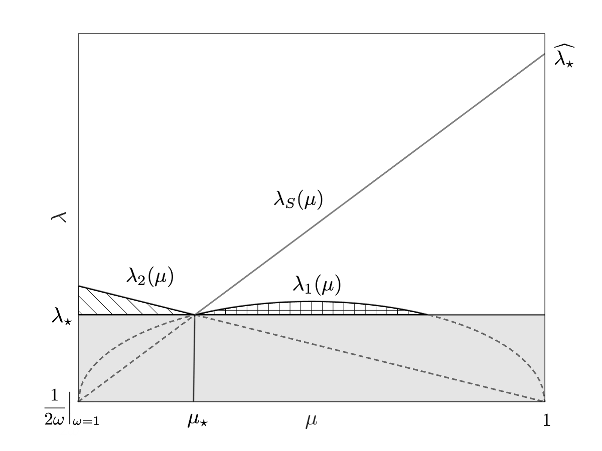
It is important to know the relative locations of various curves to optimize the time step condition. For general weight function $\omega$ , it is nontrivial to visualize these curves, yet their relative locations and some special points are captured in Figure 6.1, which is for the constant weight function $\omega\equiv 1$ . The figure can also facilitate the readers to follow and understand the analysis in this section, which is given algebraically for general $\omega$ and has a geometric interpretation for the special case of $\omega\equiv 1$ .

Refer to caption — Figure 6.1: Plots with constant $\omega\equiv 1$ to facilitate the understanding of Lemmas 6.1-6.2. The scheme is: i) unconditionally stable when $\lambda=\varepsilon/(\sigma_{m}h)$ and $\mu$ fall into the gray region, ii) $\mu$ -stable under $\Delta t\leq\tau_{\varepsilon,h,1}(\mu)$ in the stripped region, iii) $\mu$ -stable under $\Delta t\leq\tau_{\varepsilon,h,2}(\mu)$ in the latticed region, and iv) $\mu$ -stable under $\Delta t\leq\min(\tau_{\varepsilon,h,1}(\mu),\tau_{\varepsilon,h,2}(\mu))$ in the blank (white) region.

Lemma 6.4.

When $\frac{\varepsilon}{\sigma_{m}h}>\max(\lambda_{1}(\mu),\lambda_{2}(\mu))$ , both $\widehat{\tau}_{\varepsilon,h,1}(\mu)$ and $\widehat{\tau}_{\varepsilon,h,2}(\mu)$ are finite, and they satisfy

\widehat{\tau}_{\varepsilon,h,1}(\mu)=\tau_{\varepsilon,h,1}(\mu)\leq\widehat{\tau}_{\varepsilon,h,2}(\mu)=\tau_{\varepsilon,h,2}(\mu)\Longleftrightarrow\mu\leq\mu_{S}(\frac{\varepsilon}{\sigma_{m}h})\Longleftrightarrow\lambda_{S}(\mu)\leq\frac{\varepsilon}{\sigma_{m}h}.

(6.6)

Moreover, $\tau_{\varepsilon,h,1}(\mu_{S}(\frac{\varepsilon}{\sigma_{m}h}))=\tau_{\varepsilon,h,2}(\mu_{S}(\frac{\varepsilon}{\sigma_{m}h})).$

Lemma 6.5.

When restricted to $\{\mu:\frac{\varepsilon}{\sigma_{m}h}>\lambda_{2}(\mu)\}$ , $\tau_{\varepsilon,h,2}(\mu)$ is positive and monotonically decreasing. When restricted to $\{\mu\in(\frac{1}{2\omega},\min(\mu_{S}(\frac{\varepsilon}{\sigma_{m}h}),1)]:\frac{\varepsilon}{\sigma_{m}h}>\lambda_{1}(\mu)\}$ , $\tau_{\varepsilon,h,1}(\mu)$ is positive and monotonically increasing.

Proof.

The definitions of $\lambda_{j}(\mu)$ ensures $\tau_{\varepsilon,h,j}(\mu)$ is positive with $j=1,2$ for the considered $\mu$ . The monotonicity of $\tau_{\varepsilon,h,2}(\mu)$ directly comes from its being linear, and what remained will be devoted to showing the monotonicity of $\tau_{\varepsilon,h,1}(\mu)$ .

Based on the definition of $\tau_{\varepsilon,h,1}(\mu)$ in (3.12b), we know that when $\frac{\varepsilon}{\sigma_{m}h}>\lambda_{1}(\mu)$ , we have $2\varepsilon^{2}\widehat{C}_{inv}||v^{2}||_{\infty}-(1-\mu)(\mu-\frac{1}{2\omega})\sigma_{m}^{2}h^{2}>0$ , and

\displaystyle\tau^{\prime}_{\varepsilon,h,1}(\mu)=\frac{2\varepsilon^{2}h^{2}\sigma_{m}\left(2\varepsilon^{2}\widehat{C}_{inv}||v^{2}||_{\infty}-(\mu-\frac{1}{2\omega})^{2}\sigma_{m}^{2}h^{2}\right)}{(2\varepsilon^{2}\widehat{C}_{inv}||v^{2}||_{\infty}-(1-\mu)(\mu-\frac{1}{2\omega})\sigma_{m}^{2}h^{2})^{2}}.

As a result, the sign of $\tau^{\prime}_{\varepsilon,h,1}(\mu)$ , same as that of $q(\mu):=2\varepsilon^{2}\widehat{C}_{inv}||v^{2}||_{\infty}-(\mu-\frac{1}{2\omega})^{2}\sigma_{m}^{2}h^{2},$ will inform about the monotonicity of $\tau_{\varepsilon,h,1}(\mu)$ .

Consider the two roots of $q(\mu)$ , which are $\tilde{\mu}_{1,2}=\tilde{\mu}_{1,2}(\frac{\varepsilon}{\sigma_{m}h})=\frac{1}{2\omega}\mp\dfrac{\varepsilon}{\sigma_{m}h}\sqrt{2\widehat{C}_{inv}||v^{2}||_{\infty}}.$ And $q(\mu)>0$ when $\mu\in(\tilde{\mu}_{1},\tilde{\mu}_{2})$ . Note that $\tilde{\mu}_{1}<\frac{1}{2\omega}$ . One can further show that $\tilde{\mu}_{2}(\lambda)>\mu_{S}(\lambda),\;\forall\lambda>0$ as below.

	$\displaystyle\mu_{S}(\lambda)<\tilde{\mu}_{2}(\lambda)$	$\displaystyle\Longleftrightarrow\frac{1}{2\omega}+\frac{1}{2}\lambda\frac{\widehat{C}_{inv}\|\|v^{2}\|\|_{\infty}}{C_{inv}\|\|v\|\|_{\infty}}<\frac{1}{2\omega}+\lambda\sqrt{2\widehat{C}_{inv}\|\|v^{2}\|\|_{\infty}}$
		$\displaystyle\Longleftrightarrow\frac{\widehat{C}_{inv}\|\|v^{2}\|\|_{\infty}}{2C_{inv}\|\|v\|\|_{\infty}}<\sqrt{2\widehat{C}_{inv}\|\|v^{2}\|\|_{\infty}}\Longleftrightarrow{\mathcal{K}}>1.$

Hence $\left(\frac{1}{2\omega},\min(\mu_{S}(\frac{\varepsilon}{\sigma_{m}h}),1)\right]\subset(\tilde{\mu}_{1},\tilde{\mu}_{2})$ . And the monotonicity of $\tau_{\varepsilon,h,1}(\mu)$ will follow.

∎

Lemma 6.6.

Assume $\lambda>0$ .

(i)

$\lambda>\lambda_{\star}\Longleftrightarrow\lambda>\lambda_{2}(\mu_{S}(\lambda))$ .
(ii)

When $\lambda\leq\widehat{\lambda}_{\star}$ , then $\lambda>\lambda_{\star}\Longleftrightarrow\lambda>\lambda_{1}(\mu_{S}(\lambda))$ .
(iii)

When $\lambda_{\star}<\frac{\varepsilon}{\sigma_{m}h}\leq\widehat{\lambda}_{\star}$ , we have $\frac{\varepsilon}{\sigma_{m}h}>\max(\lambda_{1}(\mu),\lambda_{2}(\mu))|_{\mu=\mu_{S}(\frac{\varepsilon}{\sigma_{m}h})}$ .

Proof.

To prove (i), we proceed from the definitions of $\lambda_{2}(\mu)$ and $\mu_{S}(\lambda)$ , and get

	$\displaystyle\lambda>\lambda_{2}(\mu_{S}(\lambda))\Longleftrightarrow$	$\displaystyle\lambda>\frac{1-\frac{1}{2\omega}-\frac{1}{2}\lambda\frac{\widehat{C}_{inv}\|\|v^{2}\|\|_{\infty}}{C_{inv}\|\|v\|\|_{\infty}}}{4C_{inv}\|\|v\|\|_{\infty}}$		(6.7)
	$\displaystyle\Longleftrightarrow$	$\displaystyle\left(1+\frac{\widehat{C}_{inv}\|\|v^{2}\|\|_{\infty}}{8(C_{inv}\|\|v\|\|_{\infty})^{2}}\right)\lambda>\frac{1-\frac{1}{2\omega}}{4C_{inv}\|\|v\|\|_{\infty}}\Longleftrightarrow\lambda>\lambda_{\star}.$		(6.8)

To prove (ii), we first notice $\mu_{S}(\lambda)>\frac{1}{2\omega}$ holds when $\lambda>0$ . With $\lambda\leq\widehat{\lambda}_{\star}$ , equivalently $\mu_{S}(\lambda)\leq 1$ , we then have

	$\displaystyle\lambda>\lambda_{1}(\mu_{S}(\lambda))\Longleftrightarrow$	$\displaystyle\lambda>\sqrt{\frac{(1-\frac{1}{2\omega}-\frac{1}{2}\lambda\frac{\widehat{C}_{inv}\|\|v^{2}\|\|_{\infty}}{C_{inv}\|\|v\|\|_{\infty}})\frac{1}{2}\lambda\frac{\widehat{C}_{inv}\|\|v^{2}\|\|_{\infty}}{C_{inv}\|\|v\|\|_{\infty}}}{2\widehat{C}_{inv}\|\|v^{2}\|\|_{\infty}}}$
	$\displaystyle\Longleftrightarrow$	$\displaystyle\lambda>\left(1-\frac{1}{2\omega}-\frac{1}{2}\lambda\frac{\widehat{C}_{inv}\|\|v^{2}\|\|_{\infty}}{C_{inv}\|\|v\|\|_{\infty}}\right)\frac{1}{4C_{inv}\|\|v\|\|_{\infty}}\Longleftrightarrow\lambda>\lambda_{\star}.$		(6.9)

(iii) is a direct result of (i) and (ii) of this lemma. ∎

6.2 Proof of Theorem 3.4: unconditionally stable region, $k\geq 1$

Based on Theorem 3.3 and the definition of (unconditional) stability, the IMEX1-LDG method is unconditionally stable if and only if $\Delta t_{\textrm{stab}}(\varepsilon,h)=\infty$ , which is equivalent to

\displaystyle\frac{\varepsilon}{\sigma_{m}h}\leq\max_{\mu\in(\frac{1}{2\omega},1]}\big(\min\big(\lambda_{1}(\mu),\lambda_{2}(\mu)\big)\big).

(6.10)

Using Lemma 6.1-(i) and Lemma 6.2-(i), one has

\min\big(\lambda_{1}(\mu),\lambda_{2}(\mu)\big)=\left\{\begin{array}[]{ll}\lambda_{1}(\mu),&\textrm{if}\;\mu\leq\mu_{\star},\\ \lambda_{2}(\mu),&\textrm{if}\;\mu\geq\mu_{\star}\end{array}\right.

(6.11)

where $\mu_{\star}\in(\frac{1}{2\omega},1)$ , and the inequality (6.10) will be simplified as

\displaystyle\frac{\varepsilon}{\sigma_{m}h}\leq\max\left(\max_{\mu\in(\frac{1}{2\omega},\mu_{\star}]}\lambda_{1}(\mu),\max_{\mu\in[\mu_{\star},1]}\lambda_{2}(\mu)\right)=\max\left(\lambda_{1}(\mu_{\star}),\lambda_{2}(\mu_{\star})\right)=\lambda_{\star}.

(6.12)

This gives the result in Theorem 3.4 regarding the unconditional stability when $k\geq 1$ .

6.3 Proof of Theorem 3.4: conditionally stable region, $1\leq k\leq 9$ , $\frac{\varepsilon}{\sigma_{m}h}>\lambda_{\star}$

In this subsection, we focus on $\varepsilon$ and $h$ that satisfy $\frac{\varepsilon}{\sigma_{m}h}>\lambda_{\star}$ . For such $\varepsilon,h$ , we have $\Delta t_{\textrm{stab}}(\varepsilon,h)<\infty$ , and the IMEX1-LDG method is conditionally stable. Based on the $\mu$ -stability result in Theorem 3.3, we want to optimize the time step condition by properly choosing $\mu$ from the admissible set, hence to get $\Delta t_{\textrm{stab}}(\varepsilon,h)$ and establish the remaining result in Theorem 3.4.

6.3.1 When $\frac{\varepsilon}{\sigma_{m}h}>\widehat{\lambda}_{\star}$

We start with the simplest case, that is when $\frac{\varepsilon}{\sigma_{m}h}>\widehat{\lambda}_{\star}$ . According to Lemma 6.2-(iii), for such $\varepsilon,h$ , one has $\frac{\varepsilon}{\sigma_{m}h}>\max(\lambda_{1}(\mu),\lambda_{2}(\mu)),\forall\mu\in(\frac{1}{2\omega},1]$ , hence $\tau_{\varepsilon,h,j}(\mu)<\infty$ , $j=1,2$ , and

\Delta t_{\textrm{stab}}(\varepsilon,h)=\max_{\mu\in(\frac{1}{2\omega},1]}\min(\tau_{\varepsilon,h,1}(\mu),\tau_{\varepsilon,h,2}(\mu)).

Using the property of $\mu_{S}(\lambda)$ in Lemma 6.1, we get

\frac{\varepsilon}{\sigma_{m}h}>\widehat{\lambda}_{\star}\Leftrightarrow\mu_{S}(\frac{\varepsilon}{\sigma_{m}h})>\mu_{S}(\widehat{\lambda}_{\star})=1\Rightarrow\mu_{S}(\frac{\varepsilon}{\sigma_{m}h})\geq\mu,\quad\forall\mu\in(\frac{1}{2\omega},1].

(6.13)

Now following the comparison property in Lemma 6.4 and the monotonicity of $\tau_{\varepsilon,h,1}(\mu)$ in Lemma 6.5, we have, when $\frac{\varepsilon}{\sigma_{m}h}>\widehat{\lambda}_{\star}$ ,

\Delta t_{\textrm{stab}}(\varepsilon,h)=\max_{\mu\in(\frac{1}{2\omega},1]\cap(\frac{1}{2\omega},\mu_{S}(\frac{\varepsilon}{\sigma_{m}h})]}\tau_{\varepsilon,h,1}(\mu)=\tau_{\varepsilon,h,1}\left(\min(\mu_{S}(\frac{\varepsilon}{\sigma_{m}h}),1)\right).

6.3.2 When ${\lambda}_{\star}<\frac{\varepsilon}{\sigma_{m}h}\leq\widehat{\lambda}_{\star}$

From here on, we assume $\frac{\varepsilon}{\sigma_{m}h}\in(\lambda_{\star},\widehat{\lambda}_{\star}]$ . The relation in (6.13) implies

\mu_{S}(\frac{\varepsilon}{\sigma_{m}h})\leq 1.

(6.14)

We decompose $(\frac{1}{2\omega},1]$ into three disjoint sets $S_{j}(\varepsilon,h)$ , $j=1,2,3$ , defined as

	$\displaystyle S_{1}(\varepsilon,h)$	$\displaystyle=\left\{\mu\in(\frac{1}{2\omega},1]:\frac{\varepsilon}{\sigma_{m}h}>\max(\lambda_{1}(\mu),\lambda_{2}(\mu))\right\},$
	$\displaystyle S_{2}(\varepsilon,h)$	$\displaystyle=\left\{\mu\in(\frac{1}{2\omega},1]:\lambda_{1}(\mu)<\frac{\varepsilon}{\sigma_{m}h}\leq\lambda_{2}(\mu)\right\},$
	$\displaystyle S_{3}(\varepsilon,h)$	$\displaystyle=\left\{\mu\in(\frac{1}{2\omega},1]:\lambda_{2}(\mu)<\frac{\varepsilon}{\sigma_{m}h}\leq\lambda_{1}(\mu))\right\}.$

One can refer to Figure 6.1 to visualize the decomposition for a constant weight function $\omega\equiv 1$ . And correspondingly,

\Delta t_{\textrm{stab}}(\varepsilon,h)=\max_{\mu\in(\frac{1}{2\omega},1]}\min(\widehat{\tau}_{\varepsilon,h,1}(\mu),\widehat{\tau}_{\varepsilon,h,2}(\mu))=\max_{j=1,2,3}\Delta t_{\textrm{stab}}^{(j)}(\varepsilon,h),

where $\Delta t_{\textrm{stab}}^{(j)}(\varepsilon,h):=\max_{\mu\in S_{j}(\varepsilon,h)}\min(\widehat{\tau}_{\varepsilon,h,1}(\mu),\widehat{\tau}_{\varepsilon,h,2}(\mu)).$ Next we will calculate $\Delta t_{\textrm{stab}}^{(1)}(\varepsilon,h)$ , and then show $\Delta t_{\textrm{stab}}^{(1)}(\varepsilon,h)\geq\Delta t_{\textrm{stab}}^{(j)}(\varepsilon,h),j=2,3$ , therefore

\Delta t_{\textrm{stab}}(\varepsilon,h)=\Delta t_{\textrm{stab}}^{(1)}(\varepsilon,h).

(6.15)

Step 1: To compute $\Delta t_{\textrm{stab}}^{(1)}(\varepsilon,h)$ . When $\mu\in S_{1}(\varepsilon,h)$ , we have $\widehat{\tau}_{\varepsilon,h,1}(\mu)=\tau_{\varepsilon,h,1}(\mu)<\infty$ , $\widehat{\tau}_{\varepsilon,h,2}(\mu)=\tau_{\varepsilon,h,2}(\mu)<\infty$ . Based on the comparison result in Lemma 6.4, and the property of $\mu_{S}(\lambda)$ in Lemma 6.1, there holds

\displaystyle\min\left(\widehat{\tau}_{\varepsilon,h,1}(\mu),\widehat{\tau}_{\varepsilon,h,2}(\mu)\right)

\displaystyle=\begin{cases}\tau_{\varepsilon,h,1}(\mu),\quad&\mu\in(\frac{1}{2\omega},\mu_{S}(\frac{\varepsilon}{\sigma_{m}h})],\\ \tau_{\varepsilon,h,2}(\mu),\quad&\mu\in(\mu_{S}(\frac{\varepsilon}{\sigma_{m}h}),1].\end{cases}

(6.16)

With $\lambda_{\star}<\frac{\varepsilon}{\sigma_{m}h}\leq\widehat{\lambda}_{\star}$ , based on Lemma 6.6-(iii), we will get $\mu_{S}(\frac{\varepsilon}{\sigma_{m}h})\in S_{1}(\varepsilon,h)$ . By further using the monotonicity of $\tau_{\varepsilon,h,j}(\mu),j=1,2$ in Lemma 6.5, and the fact $\tau_{\varepsilon,h,1}(\mu_{S}(\frac{\varepsilon}{\sigma_{m}h}))=\tau_{\varepsilon,h,2}(\mu_{S}(\frac{\varepsilon}{\sigma_{m}h}))$ in Lemma 6.4, when $\frac{\varepsilon}{\sigma_{m}h}\in(\lambda_{\star},\widehat{\lambda}_{\star}]$ ,

	$\displaystyle\Delta t_{\textrm{stab}}^{(1)}(\varepsilon,h)$	$\displaystyle=\max_{\mu\in S_{1}(\varepsilon,h)}\Big(\min\left(\widehat{\tau}_{\varepsilon,h,1}(\mu),\widehat{\tau}_{\varepsilon,h,2}(\mu)\right)\Big)$
		$\displaystyle=\tau_{\varepsilon,h,1}(\mu_{S}(\frac{\varepsilon}{\sigma_{m}h}))=\tau_{\varepsilon,h,1}\left(\min(\mu_{S}(\frac{\varepsilon}{\sigma_{m}h}),1)\right).$		(6.17)

Step 2: To show $\Delta t_{\textrm{stab}}^{(2)}(\varepsilon,h)\leq\Delta t_{\textrm{stab}}^{(1)}(\varepsilon,h)$ . When $\mu\in S_{2}(\varepsilon,h)$ , we have $\widehat{\tau}_{\varepsilon,h,1}(\mu)=\tau_{\varepsilon,h,1}(\mu)<\infty$ , $\widehat{\tau}_{\varepsilon,h,2}(\mu)=\infty$ , hence $\min(\widehat{\tau}_{\varepsilon,h,1}(\mu),\widehat{\tau}_{\varepsilon,h,2}(\mu))=\tau_{\varepsilon,h,1}(\mu)$ .

For any $\mu\in S_{2}(\varepsilon,h)$ , based on Lemma 6.2, we have $\mu\leq\mu_{\star}$ . Moreover, using the fact of $\mu_{S}(\lambda_{\star})=\mu_{\star}$ and the monotonicity of $\mu_{S}(\lambda)$ in Lemma 6.1, as well as the assumption $\frac{\varepsilon}{\sigma_{m}h}>\lambda_{\star}$ , we have for $\mu\in S_{2}(\varepsilon,h)$ ,

\mu\leq\mu_{\star}=\mu_{S}(\lambda_{\star})<\mu_{S}(\frac{\varepsilon}{\sigma_{m}h}).

Finally, we can once again use the monotonicity of $\tau_{\varepsilon,h,1}(\mu)$ in Lemma 6.5, and conclude

	$\displaystyle\Delta t_{\textrm{stab}}^{(2)}(\varepsilon,h)$	$\displaystyle=\max_{\mu\in S_{2}(\varepsilon,h)}\Big(\min\left(\widehat{\tau}_{\varepsilon,h,1}(\mu),\widehat{\tau}_{\varepsilon,h,2}(\mu)\right)\Big)=\max_{\mu\in S_{2}(\varepsilon,h)}\tau_{\varepsilon,h,1}(\mu)$
		$\displaystyle\leq\tau_{\varepsilon,h,1}\left(\mu_{S}(\frac{\varepsilon}{\sigma_{m}h})\right)=\Delta t_{\textrm{stab}}^{(1)}(\varepsilon,h).$		(6.18)

Step 3: To show $\Delta t_{\textrm{stab}}^{(3)}(\varepsilon,h)\leq\Delta t_{\textrm{stab}}^{(1)}(\varepsilon,h)$ . When $\mu\in S_{3}(\varepsilon,h)$ , we have $\widehat{\tau}_{\varepsilon,h,1}(\mu)=\infty$ , $\widehat{\tau}_{\varepsilon,h,2}(\mu)=\tau_{\varepsilon,h,2}(\mu)<\infty$ , hence $\min(\widehat{\tau}_{\varepsilon,h,1}(\mu),\widehat{\tau}_{\varepsilon,h,2}(\mu))=\tau_{\varepsilon,h,2}(\mu)$ .

Given any $\mu\in S_{3}(\varepsilon,h)$ , we know $\lambda_{2}(\mu)<\frac{\varepsilon}{\sigma_{m}h}\leq\lambda_{1}(\mu)$ . This, combined with Lemma 6.2, implies $\mu>\mu_{\star}$ , and additionally

\displaystyle\frac{\varepsilon}{\sigma_{m}h}\leq\lambda_{1}(\mu)<\lambda_{S}(\mu)\Leftrightarrow\mu>\mu_{S}\left(\frac{\varepsilon}{\sigma_{m}h}\right).

(6.19)

The equivalency is based on the monotonicity of $\mu_{S}(\lambda)$ in Lemma 6.1. Finally one can use the monotonicity of $\tau_{\varepsilon,h,2}(\mu)$ in Lemma 6.5, and conclude

	$\displaystyle\Delta t_{\textrm{stab}}^{(3)}(\varepsilon,h)$	$\displaystyle=\max_{\mu\in S_{3}(\varepsilon,h)}\Big(\min\left(\widehat{\tau}_{\varepsilon,h,1}(\mu),\widehat{\tau}_{\varepsilon,h,2}(\mu)\right)\Big)=\max_{\mu\in S_{3}(\varepsilon,h)}\tau_{\varepsilon,h,2}(\mu)$
		$\displaystyle\leq\tau_{\varepsilon,h,2}(\mu_{S}(\frac{\varepsilon}{\sigma_{m}h}))=\tau_{\varepsilon,h,1}\left(\mu_{S}(\frac{\varepsilon}{\sigma_{m}h})\right)=\Delta t_{\textrm{stab}}^{(1)}(\varepsilon,h).$

7 Proof for AP property: Theorem 4.1

We will first build some preparatory results in Lemma 7.1, before proving the main result on the AP property in Theorem 4.1. The three assumptions in Section 4 still hold. Let $\{\Psi_{j}\}_{j=1}^{N_{k}}$ be an orthonormal basis of $U_{h}^{k}$ with respect to the standard $L^{2}$ inner product of $L^{2}(\Omega_{x})$ . Recall the initialization is via the $L^{2}$ projection onto $U_{h}^{k}$ , namely, $\rho^{0}_{\varepsilon,\Delta t,h}=\pi_{h}\rho_{\varepsilon}^{0}$ , $g^{0}_{\varepsilon,\Delta t,h}=\pi_{h}g_{\varepsilon}^{0}$ , $u_{\varepsilon,\Delta t,h}^{0}=\pi_{h}(\sigma_{s}^{-1}q^{0}_{\varepsilon})$ . We also define $W_{{\Delta t,h}}^{0}=\pi_{h}W_{0}$ for $W=\rho,g$ , and $u_{\Delta t,h}^{0}=\pi_{h}(\sigma_{s}^{-1}q_{0})$ .

Lemma 7.1.

The following results hold.
(i) $q_{\varepsilon}^{0}\rightharpoonup q_{0}$ in $L^{2}(\Omega_{x})$ as $\varepsilon\rightarrow 0$ .
(ii) $\lim_{\varepsilon\rightarrow 0}\rho_{\varepsilon,\Delta t,h}^{0}=\rho^{0}_{{\Delta t,h}}$ , $\lim_{\varepsilon\rightarrow 0}u_{\varepsilon,\Delta t,h}^{0}=u_{{\Delta t,h}}^{0}$ and

		$\displaystyle\lim_{\varepsilon\rightarrow 0}\langle\zeta,g_{\varepsilon,\Delta t,h}^{0}(x,\cdot)\rangle=\langle\zeta,g_{\Delta t,h}^{0}(x,\cdot)\rangle,\quad\forall\zeta\in L^{2}(\Omega_{v}),\;\;\forall x\in\Omega_{x},$		(7.1)
		$\displaystyle\lim_{\varepsilon\rightarrow 0}\langle\zeta,(g_{\varepsilon,\Delta t,h}^{0},\psi)\rangle=\langle\zeta,(g_{\Delta t,h}^{0},\psi)\rangle,\quad\forall\zeta\in L^{2}(\Omega_{v}),\;\;\forall\psi\in L^{2}({\Omega_{x}}).$		(7.2)

(iii) $\sup_{\varepsilon}||W_{\varepsilon,\Delta t,h}^{0}||<\infty$ , where $W=\rho,g,u$ .
(iv) $\sup_{\{0<\varepsilon<\varepsilon_{0}(h)\}}||W_{\varepsilon,\Delta t,h}^{1}||=C_{W}(k,\Delta t,h,{\Omega_{v}})<\infty$ , where $W=\rho,u$ .

Proof.

(i) Start with any $\phi\in C^{\infty}_{0}(\Omega_{x})$ , then

(q_{0},\phi)=-(\rho_{0},\phi_{x})=-\lim_{\varepsilon\rightarrow 0}(\rho_{\varepsilon}^{0},\phi_{x})=\lim_{\varepsilon\rightarrow 0}(q_{\varepsilon}^{0},\phi).

(7.3)

This result can be extended to any $\phi\in L^{2}(\Omega_{x})$ , hence $q_{\varepsilon}^{0}\rightharpoonup q_{0}$ in $L^{2}(\Omega_{x})$ as $\varepsilon\rightarrow 0$ , due to the uniform boundedness of $||q_{\varepsilon}^{0}||$ in $\varepsilon$ in Assumption 2 and $C^{\infty}_{0}(\Omega_{x})$ being dense in $L^{2}(\Omega_{x})$ .

(ii) With $W_{\varepsilon}^{0}$ weakly convergent to $W_{0}$ in $L^{2}(\Omega_{x})$ , for $W=\rho,q$ , we have

\lim_{\varepsilon\rightarrow 0}\rho_{\varepsilon,\Delta t,h}^{0}=\lim_{\varepsilon\rightarrow 0}\pi_{h}\rho_{\varepsilon}^{0}=\lim_{\varepsilon\rightarrow 0}\sum_{j=1}^{N_{k}}(\rho_{\varepsilon}^{0},\Psi_{j})\Psi_{j}=\sum_{j=1}^{N_{k}}\lim_{\varepsilon\rightarrow 0}(\rho_{\varepsilon}^{0},\Psi_{j})\Psi_{j}=\sum_{j=1}^{N_{k}}(\rho_{0},\Psi_{j})\Psi_{j}=\pi_{h}\rho_{0}=\rho^{0}_{\Delta t,h},

\lim_{\varepsilon\rightarrow 0}u_{\varepsilon,\Delta t,h}^{0}=\lim_{\varepsilon\rightarrow 0}\pi_{h}(\sigma_{s}^{-1}q_{\varepsilon}^{0})=\lim_{\varepsilon\rightarrow 0}\sum_{j=1}^{N_{k}}(\sigma_{s}^{-1}q_{\varepsilon}^{0},\Psi_{j})\Psi_{j}=\sum_{j=1}^{N_{k}}(\sigma_{s}^{-1}q_{0},\Psi_{j})\Psi_{j}=\pi_{h}(\sigma_{s}^{-1}q_{0})=u^{0}_{\Delta t,h}.

Now we consider any $\zeta\in L^{2}(\Omega_{v})$ . With $\langle\zeta g_{\varepsilon}^{0}\rangle$ weakly convergent to $\langle\zeta g_{0}\rangle$ in $L^{2}(\Omega_{x})$ , we have for any $x\in\Omega_{x}$ ,

	$\displaystyle\lim_{\varepsilon\rightarrow 0}\langle\zeta,g_{\varepsilon,\Delta t,h}^{0}(x,\cdot)\rangle$	$\displaystyle=\lim_{\varepsilon\rightarrow 0}\langle\zeta,\sum_{j=1}^{N_{k}}(g_{\varepsilon}^{0},\Psi_{j})\Psi_{j}(x)\rangle=\sum_{j=1}^{N_{k}}\lim_{\varepsilon\rightarrow 0}(\langle\zeta g_{\varepsilon}^{0}\rangle,\Psi_{j})\Psi_{j}(x)$
		$\displaystyle=\sum_{j=1}^{N_{k}}(\langle\zeta g_{0}\rangle,\Psi_{j})\Psi_{j}(x)=\langle\zeta,g^{0}_{\Delta t,h}(x,\cdot)\rangle.$		(7.4)

And (7.2) can be proved similarly.

(iii) Note that

|||g_{\varepsilon,\Delta t,h}^{0}|||^{2}=\langle||g_{\varepsilon,\Delta t,h}^{0}||^{2}\rangle=\langle\sum_{j=1}^{N_{k}}(g_{\varepsilon}^{0},\Psi_{j})^{2}\rangle\leq|||g_{\varepsilon}^{0}|||^{2}\sum_{j=1}^{N_{k}}||\Psi_{j}||^{2}=N_{k}|||g_{\varepsilon}^{0}|||^{2},

||u_{\varepsilon,\Delta t,h}^{0}||=||\pi_{h}(\sigma_{s}^{-1}q_{\varepsilon}^{0})||\leq||\sigma_{s}^{-1}q_{\varepsilon}^{0}||\leq\sigma_{m}^{-1}||q_{\varepsilon}^{0}||.

With Assumption 2, we have $\sup_{\varepsilon}|||W_{\varepsilon,\Delta t,h}^{0}|||<\infty,W=g,u$ . Similar proof goes to $\rho$ .

(iv) Based on (2.10), one has

	$\displaystyle(\rho_{\varepsilon,\Delta t,h}^{1},{\phi})$	$\displaystyle=\Delta t\omega\langle v^{2}\rangle l_{h}(u^{1}_{\varepsilon,\Delta t,h},{\phi})+(\rho^{0}_{\varepsilon,\Delta t,h},{\phi})$
		$\displaystyle-\Delta tl_{h}(\langle v(g^{0}_{\varepsilon,\Delta t,h}+\omega vu_{\varepsilon,\Delta t,h}^{0})\rangle,{\phi})-(\sigma_{a}\rho_{\varepsilon,\Delta t,h}^{1},{\phi}),\;\forall{\phi}\in U_{h}^{k}.$		(7.5)

Take ${\phi}=\rho_{\varepsilon,\Delta t,h}^{1}$ , use $l_{h}(u^{1}_{\varepsilon,\Delta t,h},\rho_{\varepsilon,\Delta t,h}^{1})=-(\sigma_{s}u^{1}_{\varepsilon,\Delta t,h},u^{1}_{\varepsilon,\Delta t,h})$ based on (2.17) and Assumption 3 for $\omega$ , we get when $\varepsilon<\varepsilon_{0}(h)$ ,

		$\displaystyle\|\|\rho_{\varepsilon,\Delta t,h}^{1}\|\|^{2}+(\sigma_{a}\rho_{\varepsilon,\Delta t,h}^{1},\rho_{\varepsilon,\Delta t,h}^{1})+\frac{2\sigma_{m}\Delta t}{3}\langle v^{2}\rangle\|\|u_{\varepsilon,\Delta t,h}^{1}\|\|^{2}$
	$\displaystyle\leq$	$\displaystyle(\rho^{0}_{\varepsilon,\Delta t,h},\rho^{1}_{\varepsilon,\Delta t,h})-\Delta tl_{h}(\langle v(g^{0}_{\varepsilon,\Delta t,h}+\omega vu_{\varepsilon,\Delta t,h}^{0})\rangle,\rho^{1}_{\varepsilon,\Delta t,h}).$		(7.6)

Following some standard steps to apply Cauchy-Schwarz inequality, Young inequality, inverse inequality (see, e.g. Lemma 3.9 in [11]), based on Assumption 3, we can find a constant $C(k,\Delta t,h,\Omega_{v})$ such that

		$\displaystyle\|(\rho^{0}_{\varepsilon,\Delta t,h},\rho^{1}_{\varepsilon,\Delta t,h})-\Delta tl_{h}(\langle v(g^{0}_{\varepsilon,\Delta t,h}+\omega vu_{\varepsilon,\Delta t,h}^{0},\rho^{1}_{\varepsilon,\Delta t,h})\rangle\|$
	$\displaystyle\leq$	$\displaystyle C(k,\Delta t,h,\Omega_{v})\left(\|\|\rho_{\varepsilon,\Delta t,h}^{0}\|\|+\|\|\|g_{\varepsilon,\Delta t,h}^{0}\|\|\|+\|\|u_{\varepsilon,\Delta t,h}^{0}\|\|\right)\|\|\rho_{\varepsilon,\Delta t,h}^{1}\|\|.$		(7.7)

Combining (7.6)-(7.7), with $\sigma_{a}(x)\geq 0$ , we obtain

		$\displaystyle\sup_{0<\varepsilon<\varepsilon_{0}(h)}\|\|\rho_{\varepsilon,\Delta t,h}^{1}\|\|\leq C(k,\Delta t,h,\Omega_{v})\sup_{\varepsilon}(\|\|\rho_{\varepsilon,\Delta t,h}^{0}\|\|+\|\|\|g_{\varepsilon,\Delta t,h}^{0}\|\|\|+\|\|u_{\varepsilon,\Delta t,h}^{0}\|\|)<\infty,$
		$\displaystyle\sup_{0<\varepsilon<\varepsilon_{0}(h)}\|\|u_{\varepsilon,\Delta t,h}^{1}\|\|\leq\sqrt{\frac{3}{2\sigma_{m}\Delta t\langle v^{2}\rangle}}C(k,\Delta t,h,\Omega_{v})\sup_{\varepsilon}(\|\|\rho_{\varepsilon,\Delta t,h}^{0}\|\|+\|\|\|g_{\varepsilon,\Delta t,h}^{0}\|\|\|+\|\|u_{\varepsilon,\Delta t,h}^{0}\|\|)<\infty.$

∎

We are ready to prove Theorem 4.1 on the AP property of the IMEX1-LDG method.

Proof of Theorem 4.1..

Let the mesh size $h$ be fixed.

Step 1: we first show that $\sup_{0<\varepsilon<\varepsilon_{0}(h)}||U_{\varepsilon,\Delta t,h}^{n}||<\infty$ for any $\Delta t$ , $n\geq 1$ , where $W=\rho,g,q,u$ . First note that when $\varepsilon<\varepsilon_{0}(h)$ , from Assumption 3, we have $2>\omega>\frac{2}{3}$ and $\mu=\frac{3}{4}\in(\frac{1}{2\omega},1]$ . Based on the $\mu$ -stability result in Theorem 3.3, we have

	$\displaystyle\|\|\rho_{\varepsilon,\Delta t,h}^{n+1}\|\|^{2}+\varepsilon^{2}\|\|\|g_{\varepsilon,\Delta t,h}^{n}\|\|\|^{2}+\Delta t\sigma_{m}\left(\frac{1}{4}\|\|\|g_{\varepsilon,\Delta t,h}^{n}\|\|\|^{2}+\frac{2}{3}\langle v^{2}\rangle\|\|u_{\varepsilon,\Delta t,h}^{n+1}\|\|^{2}\right)$
$\displaystyle\leq$	$\displaystyle E_{h,\mu=\frac{3}{4}}^{n+1}\leq E_{h,\mu=\frac{3}{4}}^{n}\leq\cdots\leq E_{h,\mu=\frac{3}{4}}^{1}$
$\displaystyle\leq$	$\displaystyle\|\|\rho_{\varepsilon,\Delta t,h}^{1}\|\|^{2}+\varepsilon^{2}\|\|\|g_{\varepsilon,\Delta t,h}^{0}\|\|\|^{2}+\Delta t\sigma_{M}\left(\frac{1}{4}\|\|\|g_{\varepsilon,\Delta t,h}^{0}\|\|\|^{2}+2\langle v^{2}\rangle\|\|u_{\varepsilon,\Delta t,h}^{1}\|\|^{2}\right).$	(7.8)

Moreover from (2.10b), we have $||q_{\varepsilon,\Delta t,h}^{n}||^{2}=(\sigma_{s}u_{\varepsilon,\Delta t,h}^{n},q_{\varepsilon,\Delta t,h}^{n})$ , hence $||q_{\varepsilon,\Delta t,h}^{n}||\leq\sigma_{M}||u_{\varepsilon,\Delta t,h}^{n}||$ . In combination of Lemma 7.1, the finiteness of $\sup_{0<\varepsilon<\varepsilon_{0}(h)}||W_{\varepsilon,\Delta t,h}^{n}||$ , $\forall n\geq 1$ follows for $W=\rho,g,q,u$ .

Step 2: With Lemma 7.1, we only need to establish (4.6) for any $n\geq 1$ . This is equivalent to show that for any given sequence $\{\varepsilon_{m}\}_{m=1}^{\infty}$ , satisfying $\lim_{m\rightarrow\infty}\varepsilon_{m}=0$ (we no longer emphasize that $\varepsilon$ considered here is bounded above by $\varepsilon_{0}(h)$ ), we have


		$\displaystyle\lim_{m\rightarrow\infty}W_{\varepsilon_{m},\Delta t,h}^{n}=W_{\Delta t,h}^{n},\quad W=\rho,q,u,$		(7.9a)
		$\displaystyle\lim_{m\rightarrow\infty}\langle\zeta,g_{\varepsilon_{m},\Delta t,h}^{n}(x,\cdot)\rangle=\langle\zeta,g_{\Delta t,h}^{n}(x,\cdot)\rangle,\quad\forall\zeta\in L^{2}(\Omega_{v}),\;\;\forall x\in\Omega_{x},$		(7.9b)
		$\displaystyle\lim_{m\rightarrow\infty}\langle\zeta,(g_{\varepsilon_{m},\Delta t,h}^{n},\psi)\rangle=\langle\zeta,(g_{\Delta t,h}^{n},\psi)\rangle,\quad\forall\zeta\in L^{2}(\Omega_{v}),\;\;\forall\psi\in L^{2}({\Omega_{x}}),$		(7.9c)

for some $W_{\Delta t,h}^{n}\in U_{h}^{k}$ , with $W=\rho,q,u$ , and $g_{\Delta t,h}^{n}\in G_{h}^{k}$ , $\forall n\geq 1$ . Let $W$ be any of $\rho,q,u$ . Given that $U_{h}^{k}$ is finite dimensional, the finiteness of $\sup_{m}||W_{\varepsilon_{m},\Delta t,h}^{n}||$ from Step 1 implies that there is a subsequence $\{W_{\varepsilon_{m_{r}},\Delta t,h}^{n}\}_{r=1}^{\infty}$ converging in $U_{h}^{k}$ under any norm as $r\rightarrow\infty$ . Let the limit be

W_{\Delta t,h}^{n}=\lim_{r\rightarrow\infty}W_{\varepsilon_{m_{r}},\Delta t,h}^{n},\quad W=\rho,q,u.

(7.10)

We now turn to $\{g_{\varepsilon_{m},\Delta t,h}^{n}\}_{m=1}^{\infty}$ . Note that each $g^{n}_{\varepsilon_{m},\Delta t,h}$ can be written as $g^{n}_{\varepsilon_{m},\Delta t,h}(x,v)=\sum_{j=1}^{N_{k}}\alpha_{\varepsilon_{m}}^{(j)}(v)\Psi_{j}(x)$ , with $|||g^{n}_{\varepsilon_{m}}|||=\left(\sum_{j=1}^{N_{k}}||\alpha_{\varepsilon_{m}}^{(j)}||^{2}_{L^{2}(\Omega_{v})}\right)^{1/2}$ . This, in addition to the finiteness of $\sup_{m}|||g_{\varepsilon_{m},\Delta t,h}^{n}|||$ in Step 1, indicates that $\sup_{r}||\alpha_{\varepsilon_{m_{r}}}^{(j)}||^{2}_{L^{2}(\Omega_{v})}$ is bounded for any $j=1,\cdots,N_{k}$ . As a Hilbert space, $L^{2}(\Omega_{v})$ is weakly sequentially compact, that is, $\{\alpha_{\varepsilon_{m_{r}}}^{(j)}\}_{r=1}^{\infty}$ has a subsequence which is weakly convergent in $L^{2}(\Omega_{v})$ . Without loss of generality, this subsequence is still denoted as $\{\alpha_{\varepsilon_{m_{r}}}^{(j)}\}_{r=1}^{\infty}$ , and the weak limit when $r\rightarrow\infty$ is denoted as $\alpha_{0}^{(j)}\in L^{2}(\Omega_{v})$ , $\forall j$ . We now define $g_{\Delta t,h}^{n}(x,v)=\sum_{j=1}^{N_{k}}\alpha_{0}^{(j)}(v)\Psi_{j}(x)$ . It is clear that $g_{\Delta t,h}^{n}\in G_{h}^{k}$ . For any $\zeta\in L^{2}(\Omega_{v})$ , and any $x\in\Omega_{x}$ ,

\lim_{r\rightarrow\infty}\langle\zeta,g_{\varepsilon_{m_{r}},\Delta t,h}^{n}(x,\cdot)\rangle=\sum_{j=1}^{N_{k}}\left(\lim_{r\rightarrow\infty}\langle\zeta,\alpha_{\varepsilon_{m_{r}}}^{(j)}\rangle\right)\Psi_{j}(x)=\sum_{j=1}^{N_{k}}\langle\zeta,\alpha_{0}^{(j)}\rangle\Psi_{j}(x)=\langle\zeta,g_{\Delta t,h}^{n}(x,\cdot)\rangle.

(7.11)

Furthermore, we have $\forall\zeta\in L^{2}(\Omega_{v}),\;\forall\psi\in L^{2}({\Omega_{x}}),$

\lim_{r\rightarrow\infty}\langle\zeta,(g_{\varepsilon_{m_{r}},\Delta t,h}^{n},\psi)\rangle=\sum_{j=1}^{N_{k}}\left(\lim_{r\rightarrow\infty}\langle\zeta,\alpha_{\varepsilon_{m_{r}}}^{(j)}\rangle\right)(\Psi_{j},\psi)=\langle\zeta,(g_{\Delta t,h}^{n},\psi)\rangle=(\langle\zeta g_{\Delta t,h}^{n}\rangle,\psi).

(7.12)

Use (7.10)-(7.12) for $n\geq 1$ as well as the similar result in Lemma 7.1 for $n=0$ , with $\zeta$ taken when needed as $v$ , $v{\bf 1}_{\{v>0\}}$ , $v{\bf 1}_{\{v<0\}}$ , $v\zeta(v)$ , $v\zeta(v){\bf 1}_{\{v>0\}}$ , $v\zeta(v){\bf 1}_{\{v<0\}}$ , also use the property (2.5) for $\omega$ , we have for any $n\geq 0$ ,


		$\displaystyle\lim_{r\rightarrow\infty}l_{h}(\langle v(g_{\varepsilon_{m_{r}},\Delta t,h}^{n}+\omega\|_{\varepsilon=\varepsilon_{m_{r}}}vu_{\varepsilon_{m_{r}},\Delta t,h}^{n}\rangle,{\phi})=l_{h}(\langle v(g_{\Delta t,h}^{n}+vu_{{\Delta t,h}}^{n})\rangle,{\phi}),\quad\forall{\phi}\in U_{h}^{k},$		(7.13a)
		$\displaystyle\lim_{r\rightarrow\infty}\langle\zeta,b_{h,v}(g_{\varepsilon_{m_{r}},\Delta t,h}^{n},{\psi})\rangle=\langle\zeta,b_{h,v}(g_{\Delta t,h}^{n},{\psi})\rangle,\quad\forall\zeta\in L^{2}(\Omega_{v}),\;\forall{\psi}\in U_{h}^{k}.$		(7.13b)

Now with (7.10)-(7.13) and Lemma 7.1 for the initial data, the numerical scheme (2.10) as $r\rightarrow\infty$ becomes, $\forall{\varphi},\;{\eta},\;{\phi}\,\;{\psi}\in U_{h}^{k}$


		$\displaystyle(q_{\Delta t,h}^{n+1},{\varphi})+d_{h}(\rho_{\Delta t,h}^{n+1},{\varphi})=0,$		(7.14a)
		$\displaystyle(\sigma_{s}u_{\Delta t,h}^{n+1},{\eta})=(q_{\Delta t,h}^{n+1},{\eta}),$		(7.14b)
		$\displaystyle(\frac{\rho_{\Delta t,h}^{n+1}-\rho_{\Delta t,h}^{n}}{\Delta t},{\phi})+l_{h}(\langle v(g_{\Delta t,h}^{n}+vu_{\Delta t,h}^{n})\rangle,{\phi})=\langle v^{2}\rangle l_{h}(u_{\Delta t,h}^{n+1},{\phi})-(\sigma_{a}\rho_{\Delta t,h}^{n+1},{\phi}),$		(7.14c)
		$\displaystyle(\langle\zeta\sigma_{s}g_{\Delta t,h}^{n+1}\rangle,{\psi})=\langle\zeta v\rangle d_{h}(\rho_{\Delta t,h}^{n+1},{\psi}),\quad\forall\zeta\in L^{2}(\Omega_{v}),$		(7.14d)

for $n\geq 0$ . Furthermore, (7.14a) and (7.14d) lead to

\langle(\pi_{h}(\sigma_{s}g_{\Delta t,h}^{n})+vq_{\Delta t,h}^{n},\zeta\psi)\rangle=0\quad\forall\zeta\in L^{2}(\Omega_{v}),\;\psi\in U_{h}^{k},\;\;n\geq 1.

(7.15)

With $g_{\Delta t,h}^{n}\in G_{h}^{k}$ hence $\pi_{h}(\sigma_{s}g_{\Delta t,h}^{n})+vq_{\Delta t,h}^{n}\in L^{2}({\Omega_{v}})\times U_{h}^{k}$ , (7.15) equivalently becomes

\pi_{h}(\sigma_{s}g_{\Delta t,h}^{n})=-vq_{\Delta t,h}^{n},\quad n\geq 1.

(7.16)

Moreover, from (7.14b) and (7.16), one can get $g_{\Delta t,h}^{n}+vu^{n}_{\Delta t,h}=0,n\geq 1$ , as shown below.

	$\displaystyle 0\leq\sigma_{m}\|\|\|g_{\Delta t,h}^{n}+vu^{n}_{\Delta t,h}\|\|\|^{2}$	$\displaystyle\leq\left\langle\left(\sigma_{s}(g_{\Delta t,h}^{n}+vu^{n}_{\Delta t,h}),g_{\Delta t,h}^{n}+vu^{n}_{\Delta t,h}\right)\right\rangle$
		$\displaystyle=\left\langle\left(-vq_{\Delta t,h}^{n}+vq_{\Delta t,h}^{n},g_{\Delta t,h}^{n}+vu^{n}_{\Delta t,h}\right)\right\rangle=0.$

Compare (7.14) and (7.16) with what we want in (4.7), one also needs to have $g_{\Delta t,h}^{0}+vu^{0}_{\Delta t,h}=0$ . This can be argued based on the initial data being well-prepared in Assumption 1. To see this, $\forall\zeta\in L^{2}({\Omega_{v}}),\forall\psi\in U_{h}^{k}$ , we proceed as follows,

	$\displaystyle 0$	$\displaystyle=\lim_{\varepsilon\rightarrow 0}\Big(\langle\zeta(g_{\varepsilon}^{0}+v\sigma_{s}^{-1}q_{\varepsilon}^{0})\rangle,\psi\Big)=\lim_{\varepsilon\rightarrow 0}\Big((\langle\zeta g_{\varepsilon}^{0}\rangle,\psi)+\langle v\zeta\rangle(q_{\varepsilon}^{0},\sigma_{s}^{-1}\psi)\Big)$
		$\displaystyle=(\langle\zeta g_{0}\rangle,\psi)+\langle v\zeta\rangle(q_{0},\sigma_{s}^{-1}\psi)=(\langle\zeta g_{\Delta t,h}^{0}\rangle,\psi)+\langle\zeta v\rangle(u_{\Delta t,h}^{0},\psi),$		(7.17)

and this gives $\langle\zeta(g_{\Delta t,h}^{0}+vu_{\Delta t,h}^{0},\psi)\rangle=0$ . Note that $g_{\Delta t,h}^{0}+vu_{\Delta t,h}^{0}\in L^{2}({\Omega_{v}})\times U_{h}^{k}$ , therefore (7.17) is indeed $g_{\Delta t,h}^{0}+vu_{\Delta t,h}^{0}=0$ , and we can conclude the limiting scheme in (4.7).

It is easy to see the limiting scheme (4.7) is a consistent discretization for (2.7). Its stability can be obtained similarly as Lemma 2.3, with

		$\displaystyle\|\|\rho^{n+1}_{\Delta t,h}\|\|^{2}+\Delta t\langle v^{2}\rangle\|\|u^{n+1}_{\Delta t,h}\|\|_{s}^{2}+(\sigma_{a}\rho^{n+1}_{\Delta t,h},\rho^{n+1}_{\Delta t,h})=(\rho^{n}_{\Delta t,h},\rho^{n+1}_{\Delta t,h})$
	$\displaystyle\Rightarrow$	$\displaystyle\frac{1}{2}\|\|\rho^{n+1}_{\Delta t,h}\|\|^{2}+\Delta t\langle v^{2}\rangle\sigma_{m}\|\|u^{n+1}_{\Delta t,h}\|\|^{2}\leq\frac{1}{2}\|\|\rho^{n}_{\Delta t,h}\|\|^{2}\leq\cdots\leq\frac{1}{2}\|\|\rho^{0}_{\Delta t,h}\|\|^{2}\leq\frac{1}{2}\|\|\rho_{0}\|\|^{2}.$		(7.18)

Finally, with a standard contradiction argument and the uniqueness of the solution to the system (4.7) (see Lemma 2.3), we conclude the limiting functions $\rho^{n}_{\Delta t,h},q^{n}_{\Delta t,h},g^{n}_{\Delta t,h},u_{\Delta t,h}^{n}$ are unique, and (7.9) holds for the entire sequence. In the case that the velocity space $\Omega_{v}$ is discrete, the analysis related to the convergence of $g_{\varepsilon,\Delta t,h}^{n}(\cdot,v)$ for each $v$ is just as simple as that for $\rho_{\varepsilon,\Delta t,h}^{n}$ and $q_{\varepsilon,\Delta t,h}^{n}$ , and the convergence is in a strong sense as in (4.8).

∎

References

[1] Sebastiano Boscarino, Philippe G LeFloch, and Giovanni Russo. High-order asymptotic-preserving methods for fully nonlinear relaxation problems. SIAM Journal on Scientific Computing, 36(2):A377–A395, 2014.
[2] Sebastiano Boscarino, Lorenzo Pareschi, and Giovanni Russo. Implicit-explicit Runge-Kutta schemes for hyperbolic systems and kinetic equations in the diffusion limit. SIAM Journal on Scientific Computing, 35(1):A22–A51, 2013.
[3] Russel E Caflisch, Shi Jin, and Giovanni Russo. Uniformly accurate schemes for hyperbolic systems with relaxation. SIAM Journal on Numerical Analysis, 34(1):246–281, 1997.
[4] Bernardo Cockburn and Chi-Wang Shu. The local discontinuous Galerkin method for time-dependent convection-diffusion systems. SIAM Journal on Numerical Analysis, 35(6):2440–2463, 1998.
[5] Pierre Degond. Asymptotic-preserving schemes for fluid models of plasmas. arXiv preprint arXiv:1104.1869, 2011.
[6] Giacomo Dimarco, Lorenzo Pareschi, and Vittorio Rispoli. Implicit-explicit Runge-Kutta schemes for the Boltzmann-Poisson system for semiconductors. Communications in Computational Physics, 15(5):1291–1319, 2014.
[7] Francis Filbet and Amélie Rambaud. Analysis of an asymptotic preserving scheme for relaxation systems. ESAIM: Mathematical Modelling and Numerical Analysis, 47(2):609–633, 2013.
[8] François Golse, Shi Jin, and C David Levermore. The convergence of numerical transfer schemes in diffusive regimes i: Discrete-ordinate method. SIAM journal on numerical analysis, 36(5):1333–1369, 1999.
[9] Jan S Hesthaven and Tim Warburton. Nodal discontinuous Galerkin methods: algorithms, analysis, and applications. Springer Science & Business Media, 2007.
[10] Jingwei Hu and Ruiwen Shu. On the uniform accuracy of implicit-explicit backward differentiation formulas (imex-bdf) for stiff hyperbolic relaxation systems and kinetic equations. arXiv preprint arXiv:1912.00559, 2019.
[11] Juhi Jang, Fengyan Li, Jing-Mei Qiu, and Tao Xiong. Analysis of asymptotic preserving DG-IMEX schemes for linear kinetic transport equations in a diffusive scaling. SIAM Journal on Numerical Analysis, 52(4):2048–2072, 2014.
[12] Juhi Jang, Fengyan Li, Jing-Mei Qiu, and Tao Xiong. High order asymptotic preserving DG-IMEX schemes for discrete-velocity kinetic equations in a diffusive scaling. Journal of Computational Physics, 281:199–224, 2015.
[13] Shi Jin. Asymptotic preserving (AP) schemes for multiscale kinetic and hyperbolic equations: a review. Lecture Notes for Summer School on Methods and Models of Kinetic Theory (M&MKT), Porto Ercole (Grosseto, Italy), 2010.
[14] Shi Jin, Lorenzo Pareschi, and Giuseppe Toscani. Diffusive relaxation schemes for multiscale discrete-velocity kinetic equations. SIAM Journal on Numerical Analysis, 35(6):2405–2439, 1998.
[15] Axel Klar. An asymptotic-induced scheme for nonstationary transport equations in the diffusive limit. SIAM journal on numerical analysis, 35(3):1073–1094, 1998.
[16] Axel Klar and Andreas Unterreiter. Uniform stability of a finite difference scheme for transport equations in diffusive regimes. SIAM Journal on Numerical Analysis, 40(3):891–913, 2002.
[17] Mohammed Lemou and Luc Mieussens. A new asymptotic preserving scheme based on micro-macro formulation for linear kinetic equations in the diffusion limit. SIAM Journal on Scientific Computing, 31(1):334–368, 2008.
[18] Jian-Guo Liu and Luc Mieussens. Analysis of an asymptotic preserving scheme for linear kinetic equations in the diffusion limit. SIAM Journal on Numerical Analysis, 48(4):1474–1491, 2010.
[19] Tai-Ping Liu and Shih-Hsien Yu. Boltzmann equation: micro-macro decompositions and positivity of shock profiles. Communications in mathematical physics, 246(1):133–179, 2004.
[20] Giovanni Naldi and Lorenzo Pareschi. Numerical schemes for kinetic equations in diffusive regimes. Applied mathematics letters, 11(2):29–35, 1998.
[21] Zhichao Peng. Structure-preserving discontinuous Galerkin methods for multi-scale kinetic transport equations and nonlinear optics models. PhD thesis, Rensselaer Polytechnic Institute, 2020.
[22] Zhichao Peng, Yingda Cheng, Jing-Mei Qiu, and Fengyan Li. Stability-enhanced AP IMEX-LDG schemes for linear kinetic transport equations under a diffusive scaling. 2018.
[23] Gerald C. Pomraning. The equations of radiation hydrodynamics. International Series of Monographs in Natural Philosophy, Oxford: Pergamon Press, 1973.
[24] Matthew A Reyna and Fengyan Li. Operator bounds and time step conditions for the DG and central DG methods. Journal of Scientific Computing, 62(2):532–554, 2015.

	$\displaystyle\|\langle vd_{h}(\rho_{h}^{n+1}-\rho_{h}^{n},g_{h}^{n})\rangle\|$	$\displaystyle=\|d_{h}(\rho_{h}^{n+1}-\rho_{h}^{n},\langle vg_{h}^{n}\rangle)\|=\|(q_{h}^{n+1}-q_{h}^{n},\langle vg_{h}^{n}\rangle)\|$
		$\displaystyle=\|(\sigma_{s}(u_{h}^{n+1}-u_{h}^{n}),\langle vg_{h}^{n}\rangle)\|\leq\sqrt{\langle v^{2}\rangle}\|\|\|g_{h}^{n}\|\|\|_{s}\;\|\|u_{h}^{n+1}-u_{h}^{n}\|\|_{s}.$		(5.4)

		$\displaystyle\|\langle{b_{h,v}}(g_{h}^{n}-g_{h}^{n-1},g_{h}^{n})\rangle\|$
		$\displaystyle\leq(\frac{\theta}{\sigma_{m}}+\eta)\|\|\|g_{h}^{n}-g_{h}^{n-1}\|\|\|^{2}+\frac{\sigma_{m}}{4\theta}\left\langle\sum_{i}\int_{I_{i}}(v\partial_{x}g_{h}^{n})^{2}dx\right\rangle+\frac{C_{inv}}{4\eta h}\sum_{i}\left\langle(v[g_{h}^{n}]_{i-\frac{1}{2}})^{2}\right\rangle$
		$\displaystyle\leq(\frac{\theta}{\sigma_{m}}+\eta)\|\|\|g_{h}^{n}-g_{h}^{n-1}\|\|\|^{2}+\frac{\widehat{C}_{inv}\|\|v^{2}\|\|_{\infty}}{4\theta h^{2}}\|\|\|g_{h}^{n}\|\|\|_{s}^{2}+\frac{C_{inv}\|\|v\|\|_{\infty}}{2\eta h}\left\langle\frac{\|v\|}{2}\sum_{i}[g_{h}^{n}]_{i-\frac{1}{2}}^{2}\right\rangle.$		(5.6)

		$\displaystyle\frac{1}{2\Delta t}(E^{n+1}_{h,\mu}-E^{n}_{h,\mu})+\varepsilon\left(1-\frac{C_{inv}\|\|v\|\|_{\infty}}{2\eta h}\right)\left\langle\frac{\|v\|}{2}\sum_{i}[g_{h}^{n}]_{i-\frac{1}{2}}^{2}\right\rangle$		(5.8)
		$\displaystyle+\left(\frac{\varepsilon^{2}}{2\Delta t}+\frac{1-\mu}{4}\sigma_{m}-\varepsilon(\frac{\theta}{\sigma_{m}}+\eta)\right)\|\|\|g_{h}^{n}-g_{h}^{n-1}\|\|\|^{2}+(1-\mu)\|\|\|\frac{g_{h}^{n}+g_{h}^{n-1}}{2}\|\|\|_{s}^{2}+\frac{1}{2\Delta t}\|\|\rho_{h}^{n+1}-\rho_{h}^{n}\|\|^{2}$
		$\displaystyle+\frac{\omega\langle v^{2}\rangle}{2}\|\|u_{h}^{n+1}-u_{h}^{n}\|\|_{s}^{2}-\sqrt{\langle v^{2}\rangle}\|\|\|g_{h}^{n}\|\|\|_{s}\;\|\|u_{h}^{n+1}-u_{h}^{n}\|\|_{s}+\left(\mu-\varepsilon\frac{\widehat{C}_{inv}\|\|v^{2}\|\|_{\infty}}{4\theta h^{2}}\right)\|\|\|g_{h}^{n}\|\|\|_{s}^{2}\leq 0.$

Stability-enhanced AP IMEX1-LDG method: energy-based stability and rigorous AP property

Abstract

1 Introduction

2 The IMEX1-LDG scheme

2.1 Reformulation

2.2 The IMEX1-LDG scheme

Lemma 2.1.

Proposition 2.2.

Lemma 2.3.

Proof.

2.3 Norms, inverse inequalities, and more notation

Lemma 2.4.

Proof.

3 Numerical stability

Theorem 3.1.

Definition 3.2.

Theorem 3.3.

Theorem 3.4.

Remark 3.5.

Theorem 3.6.

Remark 3.7.

4 Asymptotic preserving (AP) property

Theorem 4.1.

Remark 4.2.

5 Proof for stability: Theorem 3.1 and Theorem 3.3

Proof of Theorem 3.3..

Proof of Theorem 3.1..

6 Proof for stability: Theorem 3.4

6.1 Preliminary lemmas

Lemma 6.1.

Lemma 6.2.

Proof.

Remark 6.3.

Lemma 6.4.

Lemma 6.5.

Proof.

Lemma 6.6.

Proof.

6.2 Proof of Theorem 3.4: unconditionally stable region, k≥1k\geq 1

6.3 Proof of Theorem 3.4: conditionally stable region, 1≤k≤91\leq k\leq 9, εσm​h>λ⋆\frac{\varepsilon}{\sigma_{m}h}>\lambda_{\star}

6.3.1 When εσm​h>λ^⋆\frac{\varepsilon}{\sigma_{m}h}>\widehat{\lambda}_{\star}

6.3.2 When λ⋆<εσm​h≤λ^⋆{\lambda}_{\star}<\frac{\varepsilon}{\sigma_{m}h}\leq\widehat{\lambda}_{\star}

7 Proof for AP property: Theorem 4.1

Lemma 7.1.

Proof.

Proof of Theorem 4.1..

References

6.2 Proof of Theorem 3.4: unconditionally stable region, $k\geq 1$

6.3 Proof of Theorem 3.4: conditionally stable region, $1\leq k\leq 9$ , $\frac{\varepsilon}{\sigma_{m}h}>\lambda_{\star}$

6.3.1 When $\frac{\varepsilon}{\sigma_{m}h}>\widehat{\lambda}_{\star}$

6.3.2 When ${\lambda}_{\star}<\frac{\varepsilon}{\sigma_{m}h}\leq\widehat{\lambda}_{\star}$