BCOR5mm
\KOMAoptionDIVclassic
\KOMAoptionheadincludefalse
\KOMAoptionfootincludefalse
\KOMAoptionpagesizeauto
\recalctypearea\KOMAoptionheadingssmall
\KOMAoptionnumbersautoendperiod
\RedeclareSectionCommand[afterskip=-1em]subsection
\RedeclareSectionCommand[afterskip=-1em]subsubsection
Definition]Problem
Definition]Assumption
Definition]Annahme
Definition]Theorem
Definition]Satz
Definition]Proposition
Definition]Lemma
Definition]Corollary
Definition]Korollar
Definition]Algorithm
Definition]Algorithmus
Robust PCA via Regularized reaper
with a Matrix-Free Proximal Algorithm
Robert Beinert1 and Gabriele
Steidl1
1
TU Berlin
Straße des 17. Juni 136
10623 Berlin
Correspondence
R. Beinert:
G. Steidl:
Abstract. Principal component analysis (PCA) is known to be sensitive to outliers, so that various robust PCA variants were proposed in the literature. A recent model, called reaper, aims to find the principal components by solving a convex optimization problem. Usually the number of principal components must be determined in advance and the minimization is performed over symmetric positive semi-definite matrices having the size of the data, although the number of principal components is substantially smaller. This prohibits its use if the dimension of the data is large which is often the case in image processing.
In this paper, we propose a regularized version of reaper which enforces the sparsity of the number of principal components by penalizing the nuclear norm of the corresponding orthogonal projector. This has the advantage that only an upper bound on the number of principal components is required. Our second contribution is a matrix-free algorithm to find a minimizer of the regularized reaper which is also suited for high dimensional data. The algorithm couples a primal-dual minimization approach with a thick-restarted Lanczos process. As a side result, we discuss the topic of the bias in robust PCA. Numerical examples demonstrate the performance of our algorithm.
Keywords. Robust PCA, regularized reaper, tensor-free PCA, PCA offset, thick-restarted Lanczos algorithm
AMS subject classification. 58C05, 62H25, 65K10
1 Introduction
Principal component analysis (PCA) [Pea01] realizes the dimensionality reduction of data by projecting them onto those affine subspace which minimizes the sum of the squared Euclidean distances between the data points and their projections. Unfortunately, PCA is very sensitive to outliers, so that various robust approaches were developed in robust statistics [HR09, LR87, Tyl87a] and nonlinear optimization. In this paper, we focus on the second one.
One possibility to make PCA robust consists in removing outliers before computing the principal components which has the serious drawback that outliers are difficult to identify and other data points are often falsely labeled as outliers. Another approach assigns different weights to data points based on their estimated relevance, to get a weighted PCA [KKSZ08] or repeatedly estimate the model parameters from a random subset of data points until a satisfactory result indicated by the number of data points within a certain error threshold is obtained [FB87]. In a similar vein, least trimmed squares PCA models [PSH14, RL05] aim to exclude outliers from the squared error function, but in a deterministic way. The variational model in [CLMW11] decomposes the data matrix into a low rank and a sparse part. Related approaches such as [MT11, XCS12] separate the low rank component from the column sparse one using different norms in the variational model. Another group of robust PCA replaces the squared norm in the PCA model by the norm [KK05]. Unfortunately, this norm is not rotationally invariant, i.e., when rotating the centered data points, the minimizing subspace is not rotated in the same way. Replacing the squared Euclidean norm in the PCA model by just the Euclidean one, leads to a non-convex robust PCA model with minimization over the Stiefel or Grassmannian manifold, see, e.g. [DZHZ06, LM18, MZL19, NNSS20]. Instead of the previous model which minimizes over the sparse number of directions spanning the low dimensional subspace, it is also possible to minimize over the orthogonal projectors onto the desired subspace. This has the advantage that the minimization can be performed over symmetric positive semi-definite matrices, e.g. using methods from semi-definite programming, and the disadvantage that the dimension of the projectors is as large as the data now. This prohibits this approach for many applications in particular in image processing. The projector PCA model is still non-convex and a convex relaxation, called reaper, was recently proposed by Lerman et el. [LMTZ15].
In this paper, we build up on the advantages of the convex reaper model, but modify it in two important directions: (i) by penalizing the nuclear norm of the approximated projectors, our model does only require an upper bound on the dimension of the desired subspace. Having the same effect as the sparsity promotion of the 1-norm, the nuclear norm – the 1-norm of the eigenvalues – promotes low-rank matrices or, equivalently, sparse eigenvalue decompositions; (ii) by combining primal-dual minimization techniques with a thick-restarted Lanczos process, we are able to handle high dimensional data. We call our new model rreaper. We provide all computation steps leading to a provable convergent algorithm and give a performance analysis following the lines of [LMTZ15]. The choice of the offset in robust PCA is an interesting problem which is not fully discussed in the literature so far. Usually, the geometric median is used. We do not provide a full solution of this issue, but show that under some assumptions the affine hyperplane in having the smallest Euclidean distance to given data points goes through of these points. We underline our theoretical findings by numerical examples.
The outline of this paper is as follows: preliminaries from linear algebra and convex analysis are given in in Section 2. In Section 3, we introduce our regularized reaper model. The basic primal-dual algorithm for its minimization is discussed in Section 4. The algorithm is formulated with respect to the full projection matrix. The matrix-free version of the algorithm is given in Section 5. It is based on the thick-restarted Lanczos algorithm and is suited for high-dimensional data. In Section 6, we examine the performance analysis of rreaper along the lines of [LMTZ15]. Some results on the offset in robust PCA are proved in Section 7. The very good performance of rreaper in particular for high dimensional data is demonstrated in Section 8. Section 9 finishes the paper with conclusions and directions of future research.
2 Notation and preliminaries
Throughout this paper we will use the following notation and basic facts from linear algebra and convex analysis which can be found in detail in various monographs and overview papers as [Bec17, BSS16, CP16, GV13, Roc70].
Linear algebra.
By we denote the Euclidean vector norm and by the norm which sums up the absolute vector components. Recall that for any ,
| (1) |
Let resp. be the vectors having entries , resp., . Analogously, we write and for the all-one and all-zero matrix in . Further, is the identity matrix. Let denote the trace of the quadratic matrix , i.e., the sum of its eigenvalues. On the Hilbert–Schmidt inner product is defined by
and the corresponding so-called Frobenius norm by .
Let denote the linear subspace of symmetric matrices. For two symmetric matrices , we write if is positive semi-definite. Every has a spectral decomposition
where denotes the vector containing the eigenvalues of in descending order and is the orthogonal matrix having the corresponding orthogonal eigenvectors as columns. The nuclear norm (trace norm) of is given by
The trace and Frobenius norm correspond to the Schatten 1-norm and 2-norm respectively, where the Schatten -norm with of a symmetric matrix is defined by . Recall that is an orthogonal projector if and . This is equivalent to the statement that and has only eigenvalues in . The nuclear norm is the unique norm such that
for every orthogonal projector .
For a given norm on , the dual norm is defined by
In particular, for a matrix we will be interested in the norm
which can be considered as norm on by arranging the columns of the matrix into a vector. Its dual norm is given by
Convex analysis.
Let denote the space of proper, lower semi-continuous, convex functions mapping from into the extended real numbers . The indicator function of is defined by
We have if and only if is non-empty, convex and closed.
For , the proximal mapping is defined by
Indeed, the minimizer exists and is unique [Roc70, Thm 31.5]. If is a nonempty, closed, convex set, then the proximal mapping of a multiple of is just the orthogonal projection onto , i.e.,
In particular, the orthogonal projection onto the halfspace with and can be computed by
where . Further, the orthogonal projection onto the hypercube is given by
| (2) |
The Fenchel dual of is the function defined by
The dual function of a norm is just the indicator function of the unit ball with respect to its dual norm. In particular, we have for that
| (3) |
where .
3 Regularized reaper
Given data points , the classical PCA finds a -dimensional affine subspace , , by minimizing
| (4) |
over and . It is not hard to check that the affine subspace goes through the offset (bias)
| (5) |
Therefore, we can reduce our attention to data points , , which we denote by again, and minimize over the linear -dimensional subspaces through the origin, i.e.,
where .
Unfortunately, the solution of this minimization problem is sensitive to outliers. Therefore several robust PCA variants were proposed in the literature. A straightforward approach consists in just skipping the square in the Euclidean norm leading to
| (6) |
This is a nonconvex model which requires the minimization over matrices in the so-called Stiefel manifold,
Another approach is based on the observation that is the orthogonal projector onto the linear subspace spanned by the columns of . Since the linear subspace is -dimensional, exactly eigenvalues of have to be one. Thus, problem (6) can be reformulated as
| (7) |
Having computed , we can determine by spectral decomposition. Unfortunately, (7) is still a nonconvex model which is moreover NP hard to solve. Therefore Lerman et al. [LMTZ15] suggested to replace it by a convex relaxation, called reaper,
In order to deal with the non-differentiability of the objective function, Lerman et al. [LMTZ15] iteratively solve a series of positive semi-definite programs. In contrast to models minimizing directly over , algorithms for minimizing reaper or rreaper seem to require the handling of a large matrix or, more precisely, the handling of its spectral decomposition which makes the method not practicable for high-dimensional data.
The above model requires the exact knowledge of the dimension of the linear subspace the data will be reduced to. In this paper, we suggest to replace the strict trace constraint by a relaxed variant and to add the nuclear norm of as a regularizer which enforces the sparsity of the rank of :
| (8) |
Here is an appropriately fixed regularization parameter.
Since (8) is again hard so solve, we use a relaxation for the eigenvalues and call the new model regularized reaper (rreaper):
| (9) |
Finally, we project the solution of rreaper to the set of orthoprojectors with rank not larger than :
where
In the following we will present a primal-dual approach to solve (9) which uses only the sparse spectral decomposition of , but not the matrix itself within the computation steps.
4 Primal-dual algorithm
rreaper is a convex optimization problem; so we may choose from various convex solvers. Since both – data fidelity and nuclear norm – are non-differentiable, we apply the primal-dual method of Chambolle and Pock [CP16]. For this purpose, we define the forward operator
and rearrange (9) as
| (10) |
where the regularizer is defined by
| (11) |
Since is compact and convex, and since the norms and are continuous, rreaper has a global minimizer. This minimizer is in general not unique. Concerning the adjoint operator , we observe
for all and , where we exploit the symmetry of by . Thus, the adjoint is just
The operator norm of is given by the spectral norm of , i.e.
In more detail, for , we obtain
Here the inequality becomes sharp for , where arises from the singular value decomposition with descending ordered singular values .
Next, we apply the primal-dual method of Chambolle and Pock [CP16] with extrapolation of the primal variable to compute the minimizer of rreaper (10), which leads us to the following numerical method.
[Primal-Dual Algorithm] Input: , and with , and
.
Intialization: ,
.
Interation:
More generally, Chambolle and Pock [CP16] have proven that the sequence converges to a minimizer of (10) and the sequence to a minimizer of the dual problem
if the Lagrangian
has a saddle-point which is, however, clear for rreaper.
The algorithm requires the computation of the proximal mapping of the dual data fidelity and of the regularizer which we consider next.
[Proximal mapping of the dual data fidelity] For and , we have
Proof 1.
For the maximal dimension of the target subspace, we henceforth use the half-space
in order to bound the trace of the primal iteration variable . Then the proximal mapping of the regularizer is given in the following proposition.
[Proximal mapping of the regularizer] For with spectral decomposition and in (11) it holds
Proof 2.
A symmetric matrix is in if and only if . Hence the regularizer can be written as
and
| (12) |
By the theorem of Hoffmann and Wielandt [HJ91, Theorem 6.3.5], we know that
with equality if and only if possesses the same eigenspaces as . Therefore, the minimizer in (12) has to be of the form , where the columns of are the eigenvectors of . Incorporating this observation in (12), we determine the eigenvalues by solving the minimization problem
Alternatively to the proof we could argue with the so-called spectral function related to which is invariant under permutations, see, e.g. [Bec17].
By Proposition 4 the proximal mapping of the regularizer requires the projection onto the truncated hypercube. The following proposition can be found in [Bec17, Ex 6.32].
[projection onto the truncated hypercube] For any and any , the projection to the truncated hypercube is given by
where is the positive root of the function
| (13) |
Due to the projection to the hypercube, see (2), only the positive components of influence its projection onto . More precisely, we have
where the function is employed componentwise.
To formulate a projection algorithm, in particular, to compute the zero of , we study the properties of .
[Properties of ] For fixed with , the function defined in (13) has the following properties:
- i)
is Lipschitz continuous.
- ii)
There exists , and such that for and for . Further, we have piecewise linearity
where
In particular, the function is monotone decreasing.
- iii)
The positive zero of is given by
Proof 3.
i) Using the definition of , the Cauchy–Schwarz inequality, and the nonexpansiveness of the projection, we get
ii) By definition of and by the assumption , we have . Starting with , we construct with iteratively as follows: given with , we set and choose
where
Here we use the convention . Note that at least one of the above sets in the definition of and is non-empty since otherwise all components of have to be non-positive implying and thus , a contradiction.
Considering the projection to the hypercube in (2), we see that the index set does not change for and that a change appears exactly in , where at least one component enters or leaves the interval . Hence we have
Let be the first value in this procedure, where . Since each component in can at most one times enter or leave the interval , we know that . Further, we have since our piecewise linear function cannot pass zero in the interval otherwise.
iii) Now the zero of in the interval can be computed by solving
which results in and finishes the proof.
Following Proposition 4 and the previous proof, we obtain the following algorithm for the projection onto .
[Projection onto truncated hypercube] Input: , .
- 1.
Compute by (2).
If , then return ;
otherwise set , and . - 2.
Repeat until :
- (a)
,
- (b)
,
- (c)
,
- (d)
,
- (e)
,
- (f)
,
- (a)
- 3.
Compute
- (a)
,
- (b)
- (a)
Output: .
5 Matrix-free realization
Solving rreaper with the primal-dual §4 is possible if the dimension of the surrounding space is moderate which is often not the case in image processing tasks. While the dual variable matches the dimension of the data, the primal variable is in instead of , . How can the primal-dual iteration be realized in the case though the primal variable cannot be hold in memory and the required eigenvalue decomposition cannot be computed in a reasonable amount of time?
Here the nuclear norm in rreaper that promotes low-rank matrices comes to our aid. Our main idea to derive a practical implementation of the primal-dual iteration is thus based on the assumption that the iterates of the primal variable possess the form
| (14) |
with small rank . In our simulations, we observed that the rank is usually around the dimension of the wanted low-dimensional subspace.
In order to integrate the matrix-free representation (14) into the primal-dual iteration efficiently, we further require a fast method to compute the eigenvalue thresholding. For this, we compute a partial eigenvalue decomposition using the well-known Lanczos process [Lan50]. Deriving matrix-free versions of the forward operator and its adjoint , we finally introduce a complete matrix-free primal-dual implementation with respect to .
5.1 The thick-restarted Lanczos process
One of the most commonly used methods to extract a small set of eigenvalues and their corresponding eigenvectors of a large symmetric matrix is the Lanczos method [Lan50]. The method builds a partial orthogonal basis first and then uses a Rayleigh–Ritz projection to extract the wanted eigenpairs approximately. If the set of employed basis vectors is increased, the extracted eigenpairs converge to the eigenpairs of the given matrix [GV13]. Since the symmetric matrix whose partial eigenvalue decomposition is required in the primal-dual method usually is high-dimensional, we would like to chose the number of basis vectors within the Lanczos method as small as possible. To calculate the dominant eigenpairs with high accuracy nevertheless, the Lanczos method can be restarted with the dominant Ritz pairs. For our purpose, we use the thick-restart scheme of Wu and Simon [WS00] in Algorithm 5.1, whose details are discussed below.
[Thick-restarted Lanczos process [WS00, Alg 3]] Input: , , .
- 1.
Choose a unit vector . Set .
- 2.
Lanczos process:
1. Initiation:
- (a)
,
- (b)
,
- (c)
,
- (d)
,
- (e)
.
2. Interation ():
- (a)
,
- (b)
,
- (c)
,
- (d)
,
- (e)
.
- (a)
- 3.
Compute the eigenvalue decomposition of in (15). Set .
- 4.
If for ,
then return and .
Otherwise, set , , and continue with (ii).
Output: , with .
Remark \theDefinition.
Although the Lanczos process computes an orthogonal basis , the orthogonality is usually lost because of the floating-point arithmetic. In order to re-establish the orthogonality, we therefore have to orthogonalize the newly computed with the previous basis vectors, which can be achieved by the Gram–Schmidt procedure. More sophisticated re-orthogonalization strategies are discussed in [WS00].
Remark \theDefinition.
During the Lanczos process, the norm of the residual could become zero. In this case, we can stop the process, reduce to the current , and proceed with step (iii) and (iv). Then the computed basis spans an invariant subspace of such that the eigenpairs in and become exact, see [GV13].
The heart of the Lanczos method in §5.1 is the construction of an orthonormal matrix such that becomes tridiagonal, see (15) with below. Using the eigenvalue decomposition , we then compute the Ritz pairs , where are the columns of and the eigenvalues in . In the next iteration, we chose Ritz pairs corresponding to the absolute leading Ritz values denoted by and restart the Lanczos process. Thereby, the chosen Ritz vectors are extended to an orthogonal basis fulfilling
| (15) |
where with and originating from the last iteration, see [WS00].
The stopping criteria of the thick-restarted Lanczos process is here deduced from the fact that the chosen Ritz pairs fulfil the equation
where is the last residuum vector of the previous iteration [WS00]. Consequently, the absolute error of the chosen Ritz pairs is given by
Usually, the absolute value of the leading Ritz value is a good approximation of the required spectral norm to estimate the current relative error.
5.2 Matrix-free primal update
The thick-restarted Lanczos method allow us to compute the leading absolute eigenvalues and their corresponding eigenvectors in a matrix-free manner using only the action of the considered matrix. In our primal-dual method for rreaper, we need the action of . Incorporating the low-rank representation (14), we see that this can be rewritten as
For the evaluation of the primal proximal mapping, we first compute the eigenvalue decomposition of , next shift the eigenvalues, and finally project them to the truncated hypercube , see §4. Since the projection onto is independent of negative eigenvalues, see note after Proposition 4, it is thus sufficient to compute only the eigenpairs with eigenvalue larger than .
For the numerical implementation, we compute the relevant eigenpairs with the thick-restarted Lanczos method. In the course of this, we are confronted with the issue that we actually do not know how many eigenpairs has to be computed. To reduce the overhead of §5.1 as much as possible, the parameters and can be easily adapted between the restarts. Further, the computation of strongly negative eigenvalues can be avoided by an eigenvalue shift, i.e. actually compute the eigenpairs of with , where the required action has the form
| (16) |
Essentially, we may thus implement the primal proximation in the following manner.
[Matrix-free primal proximation] Input: , , , , .
- 1.
- 2.
Projection onto :
Run §4 on
to get . - 3.
New low-rank representation:
Determine and return .
Output: .
Remark \theDefinition.
If the matrix does not possess any eigenvalues greater than , then the Lanczos process stops in step (i.a) with . Since the projection to the truncated hypercube is then the zero vector again, the new iteration can be represented by an empty low-rank representation, i.e. .
5.3 Matrix-free dual update
Compared with the primal update, the derivation of the matrix-free dual update is more straightforward. First, the matrix
is computed, where the over-relaxation is already plugged in. The low-rank representations of and similar to (14) can efficiently incorporated by calculating the matrix column by column. This way of handling the forward operator nicely matches with the projection of the columns to the Euclidean unit ball in the second step. Writing the matrix column by column too, we obtain the following numerical method.
[Matrix-free dual proximation] Input: , , , , .
- 1.
For , compute
- 2.
For , compute .
- 3.
Return .
Output:
5.4 Matrix-free projection onto the orthoprojectors
With the matrix-free implementations of the primal and dual proximal mappings, we are already able to solve rreaper (9) numerically. Before summarizing the compound algorithm, we briefly discuss the last needed component to tackle the robust PCA problem (8). The final step is to project the solution of rreaper onto the set of orthoprojectors with rank not larger than :
where
We may calculate the projection explicitly in the following manner.
[Projection onto the orthoprojectors] For with eigenvalue decomposition , and for every , the projection onto with respect to the Schatten -norm is given by
Proof 4.
The key ingredient to prove this statement is the theorem of Lidskii–Mirsky–Wielandt, see for instance [LM99]. Using this theorem to estimate the Schatten -Norm, we obtain
| (17) |
where we have equality if has the same eigenvectors as . Recall that the eigenvalues in appear in descending order. The right-hand side of (17) thus becomes minimal if we choose the eigenvalues of for as
and set for . This is exactly the projection onto .
Because of the low-rank representation of the primal variable, the construction of the orthoprojector is here especially simple.
[Matrix-free projection onto orthoprojectors] Input: , .
- 1.
Projection onto :
Determine . - 2.
Matrix-free presentation:
Return .
Output: .
5.5 Matrix-free robust PCA by rreaper
Combining the matrix-free implementations of the primal and dual proximal mappings, we finally obtain a primal-dual method to solve rreaper (9) without evaluating the primal variable representing the relaxed orthoprojector explicitly.
6 Performance analysis
Inspired by ideas of Lerman et al. [LMTZ15], we examine the performance analysis of rreaper. To this end, we assume that the ‘ideal’ subspace of the given data , has dimension . As in [LMTZ15], we determine the best fit of the data by two measures: the first one is the distance of the data from the subspace
where denotes the orthogonal projector onto . For the second measure, we assume that the projected data , , form a frame in meaning that there exist constants such that
for all with . In order to recover the entire subspace , the data have obviously to cover each direction in with sufficiently many data points. This well-localization of the data is measured by the permeance statistic
| (18) |
which can be seen as counterpart of the lower frame bound. Clearly, becomes large if all direction in are uniformly covered by the data. The lower frame bound and the permeance statistic come into the play in the following lemma, compare with [LMTZ15, Section A2.3].
Let be the orthogonal projector onto a subspace of of dimension and , , which form the columns of the matrix . Then, for any , the following relations hold true:
| (19) |
and
| (20) |
Proof 5.
We restrict our attention to (20). The relation (19) follows similar lines. Let have the singular value decomposition , where the singular values , are in descending order and and we can arrange such that the transpose of the first rows of belong to . Then it holds
Using orthogonality of and concavity of the square root function, we obtain
Now we can estimate the reconstruction error of rreaper.
Let be the orthogonal projector onto a subspace of of dimension and , , such that their projections onto form a frame of . Define by (18) and set . Let be the solution of (9) and the projection of onto . Then, for the reconstruction error is bounded by
Proof 6.
Since is a minimizer of (9), we obtain
| (21) | ||||
| (22) |
It remains to estimate from below. To this end, we decompose as
Since , we obtain be conjugation with , resp. that and , so that and . Then we conclude
which implies
Now we can estimate the last summand by (1) and Lemma 6 as
| (23) |
| (24) | ||||
Using that by the triangular inequality
we get
Now we can use the estimate to get
if . The final assertion follows by
7 Incorporating the offset
So far, we have assumed that the offset in the robust PCA problem is given, so that we can just search for a low dimensional linear subspace which represents the data well. While in the classical PCA (4) the affine subspace always passes trough the mean value (5) of the data, it is not clear which value must be chosen in order to minimize
| (25) |
Clearly, if is a minimizer of , then, for every , also is a minimizer.
A common choice for the offset is the geometric median of the data points defined by
which can be computed e.g. by the Weiszfeld algorithm and its generalizations, see, e.g. [BS15, OJ78, SST12, Wei37]. Other choices arising, e.g. from Tylor’s M-estimator or other robust statistical approaches [KTV94, LNNS19, LM18, MVD97, Tyl87b], were proposed in the literature. However, they do in general not minimize (25) as the following example from [NNSSar] shows: given three points in which form a triangle with angles smaller than 120 degrees, the geometric median is the point in the inner of the triangle from which the points can be seen under an angle of 120 degrees. In contrast, the line () having smallest distance from the three points is the one which passes through those two points with the largest distance from each other.
In the following, we show that there always exists an optimal hyperplane of dimension in determined by a minimizer of in (25) that contains at least data points. Further, if the number of data points is odd, then every optimal hyperplane contains at least data points. Recall that the hyperplane spanned by the columns of with offset is given by
where , is a unit normal vector of the hyperplane, which is uniquely determined up to its sign and .
The following lemma describes the placement of the data points with respect to the halfspaces determined by a minimizing hyperplane.
Let , . Let be a minimizer of and with
Then it holds . In particular, it holds if is odd. Also for even there exists a minimizing hyperplane with for some .
Proof 7.
W.l.o.g. assume that . If , then all data points are in the mimimizing hyperplane and we are done. Otherwise, the value is positive, and we consider the shifted hyperplane , which contains at least one data point. The sum of the distances of the data points from this hyperplane is
Since is a minimizer of this implies that . If , then and the shifted hyperplane is also minimizing. However, this case cannot appear for odd so hat for odd . This finishes the proof.
Let , . Then there exists a minimizer of such that the corresponding minimizing hyperplane contains at least data points. If is odd, every minimizing hyperplane contains at least data points.
Proof 8.
By Lemma 7 there exists a data point such that with is a minimizer of and for odd every minimizing hyperplane passes through a data point. Let be a unit vector orthogonal to the columns of . Set , . Next, we show: if the subspace normal to contains linearly independent vectors with , then exactly one of the following situations apply. (i) The remaining vektors with are linearly dependent from the first vectors and thus in the same linear subspace . (ii) We find a further independent vector, say , contained in the subspace normal to such that we can increase to . Repeating this argumentation until , we are done since , and itself are in the subspace corresponding to .
Because the vectors with are independent and are contained in the subspace normal to by assumption, there exists a matrix
with , whose first columns have the same span as , i.e.
This especially implies for and . Note that the normal unit vector of is also , and that the objectives coincides, i.e.
| (26) |
Now, let the matrix-valued function be defined by
where the three building factors are given by
Figuratively, the function takes the orthonormal columns of and rotates the last vektor by the angle in the plane spanned by and . Clearly, we have . Due to (26), the function
has moreover a minimum in . For the summands of , we obtain
since and are orthogonal by construction. Hence, we get
Here the first summands vanish because of the mentioned orthogonality and for .
If all remaining given points with are in , then the corresponding remaining summands of become zero too, and the first situation (i) applies; so we are done.
If this is not the case, consider only those with that are linearly independent of the , . Let us denote the corresponding non-empty index set by . Assume that there exists a such that is not differentiable in . This is only possible if the argument of the absolute value vanishes implying
Thus, the vector is in the subspace spanned by the columns of , and we are done. Otherwise, if for all , then it is differentiable in and, by straightforward differentiation, we obtain
But then cannot be a minimizer of which is a contradiction. Hence, this case cannot occur and the proof is complete.
If the target dimension of the minimizing subspace is strictly less than , then it does not have to contain any data point as the following example shows.
Counterexample \theDefinition (Lower-dimensional subspace approximation).
Initially, we consider the approximation of some given points in by an one-dimensional subspace – a line. More precisely, for a fixed , we consider the six given points
We thus have two well-separated clusters around and .
Obviously, the optimal line has somehow to go through each cluster. One possible candidate for the approximation line is simply the axis , whose distance to the given points is by construction – for each cluster . Now, assume that the line goes through one given point, say . If is very large, then we can neglect the slope of the line. Only considering the distances within the cluster around , we notice that the distance increases from to approximately . Although the axis is maybe not the optimal line, the distance to the given points is smaller than for a line going through a data point. Therefore, we can conclude that the optimal line has not to contain any given point.
The same construction can be done for arbitrary subspaces of dimension . For example, consider just the points
where is the th unit vector. Using the same argumentation as above, the distance to the subspace is smaller than to any -dimensional subspace containing at least one data point.
8 Numerical examples
In this section, we demonstrate the performance of rreaper by numerical examples implemented in MATLAB.
8.1 (2,1)-norm versus Frobenius norm
This example with simple synthetic data will show that the (2,1)-norm in the data term is more robust against outliers than the Frobenius norm
For the Frobenius norm here abbreviated as -norm, we have only to replace the projection onto with the projection to the Frobenius norm ball
We want to recover a line in the plane. Since this recovery problem is invariant under rotations, we restrict ourselves to . The data are generated randomly and consist of 50 points near the considered axis – we added a small amount of noise in the second coordinate – and of 10 outliers located somewhere in the plane, see Figure 1.
Besides the data points, the recovered lines using rreaper with the (2,1)-norm (solid line) as data fidelity and the Frobenius norm (dashed line) with parameters and are presented. In this toy example, rreaper yield nearly a perfect result regardless of the outliers, and is in particular more robust than the same model with the Frobenius norm.
8.2 Nuclear norm and truncated hypercube constraints
In this example we are interested how the rank reduction is influenced by the nuclear norm and the projection to the truncated hypercube. In this synthetic experiment, we approximate the given data by a 10-dimensional subspace. The data is again generated randomly, where 100 points lie near the subspace spanned by the first ten unit vectors and additional 25 outliers. In Figure 2.a, the dataset is represented by the distance to the subspace and to the orthogonal complement .
We apply rreaper in §5.5 with different parameter combination. For the target dimension, we choose in our first experiment , which is the wanted dimension, and second one , which does not truncate the unit hypercube at all. The influence of the regularization parameter on the rank of is shown in Figure 2.b, where the lines from top to down correspond to the regularization parameters . Since we start the iteration with the zero-rank matrix , the first iterations for and coincides up to the point, where the trace of exceeds the value 10.
Considering only the results for (solid lines), we see that the nuclear norm reduces the rank of the iteration variable with an increasing regularization parameter. Further, the rank during the primal-dual algorithm is very sensitive to the regularization parameter. For (dashed lines), the situation changes dramatically. After the initial stages, the rank of decreases nearly to the target dimension. Since the matrices are no orthogonal projections, rank and trace do not conincide. Due to this fact, the rank is not strictly bounded by the maximal trace of the truncated hypercube. Nevertheless, the projection to the truncated hypercube significantly reduces the rank.
For an optimal rank evolution during the matrix-free primal-dual method, the projection to the truncated hypercube by §4 appers to be important. Moreover, the projection makes the rank evolution less sensitive to the regularization parameter so that a wider range of regularization parameters can be applied without lossing the computational benefits of the low rank. Thus, the truncated hypercube projection is an elementary key component of the algorithm.
8.3 Face approximation
The idea to use the principle components of face images – the so-called eigenfaces – for recognition, classification, and reconstruction was considered in various paper and goes probably back to [TP91]. In this experiment, we adopt this idea to show that our matrix-free reaper can handle high-dimensional data. Since the computation of an optimal offset is non-trivial as discussed in Section 7, we choose just the geometric median.
For the first experiment, we use the cropped ‘Extended Yale Face Dataset B’ [GBK01, LHK05]. The considered part of the dataset consists in 64 images with 168192 pixels with integer values between 0 and 255 of one face under different lighting conditions, but with the same facial expression, see Figure 3.a.
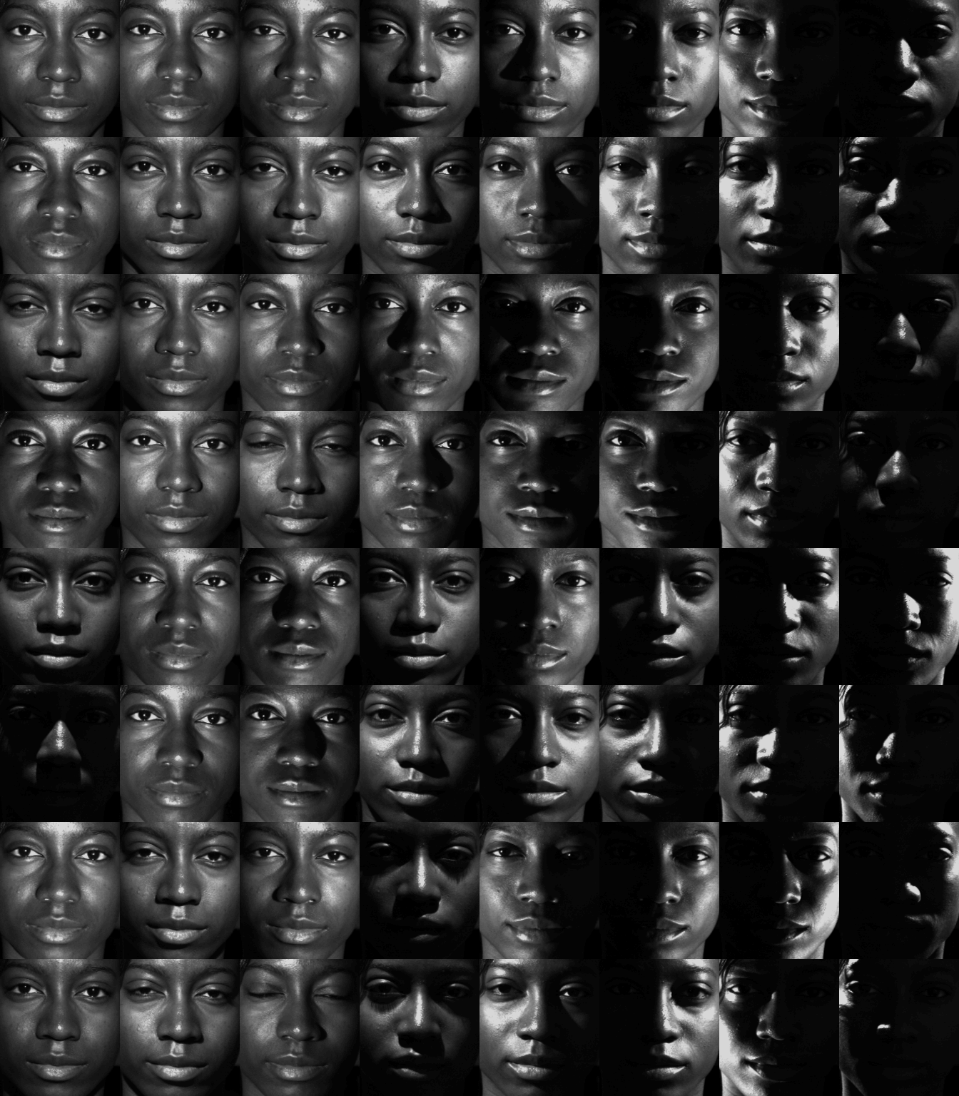
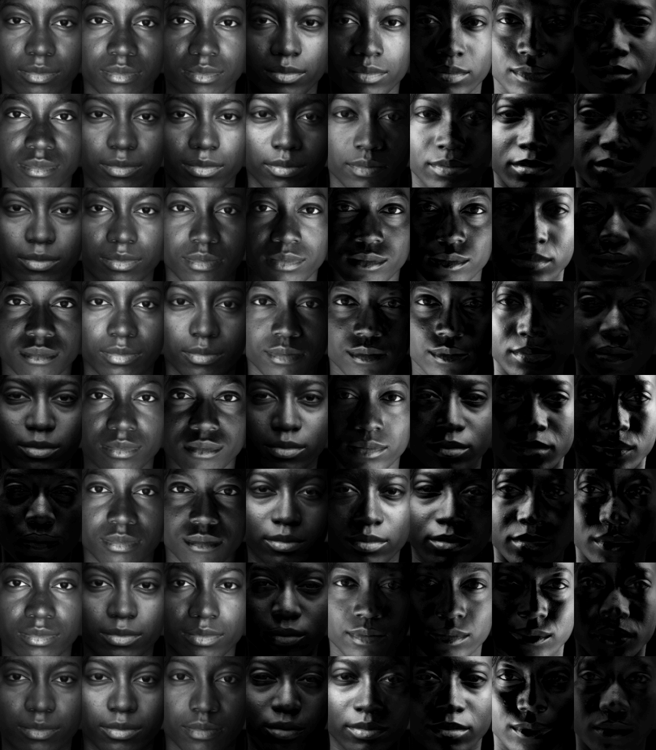
It is well-known that such images can be well approximated by a subspace covering around five directions [EHY95]. In our simulation, we set the maximal dimension to . For the chosen regularization parameter , our matrix-free rreaper finds a seven-dimensional subspace. The projection of the original data to this subspace is shown in Figure 3.b – a higher resolved example in Figure 4.a.


An typical effect of the projection to the low-dimensional subspace is that dark regions are lightened, shadows are removed, and reflections at skin and eyes are cleared away. The recovered subspace learned from uncorrupted face images can be used to remove corrupted parts in additional images as shown in Figure 4.b.
In our second experiment, we consider images with a higher resolution. The main motivation to develop a matrix-free algorithm have been to handle such data. We apply rreaper to determine a five-dimensional subspace form the full Extended Yale Face Dataset B. The used dataset is shown in Figure 5, where each image has 640480 pixels. Notice that an artefact has been placed in the first four images covering the right eye, the nose, the right ear, and the mouth respectively.
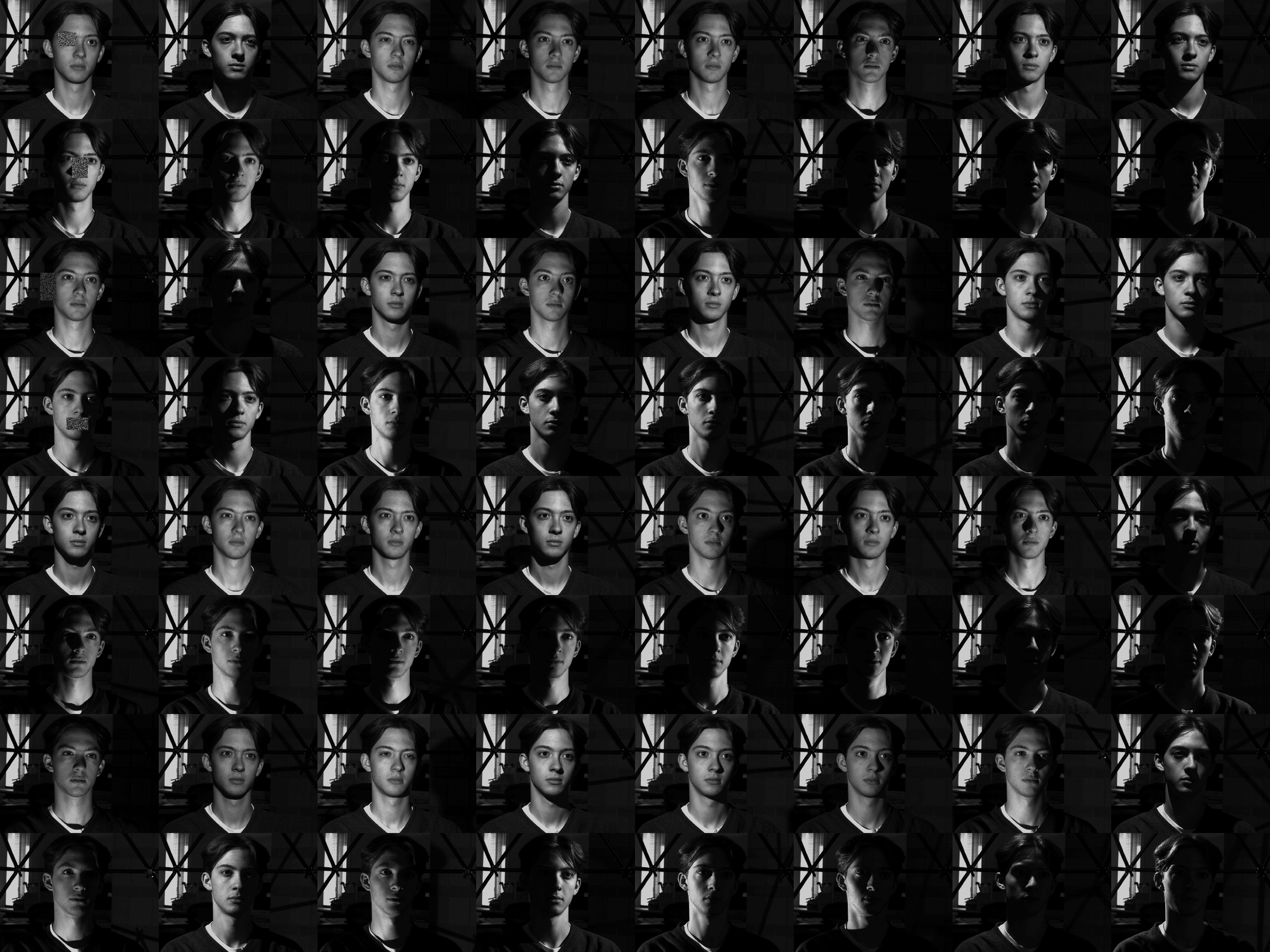
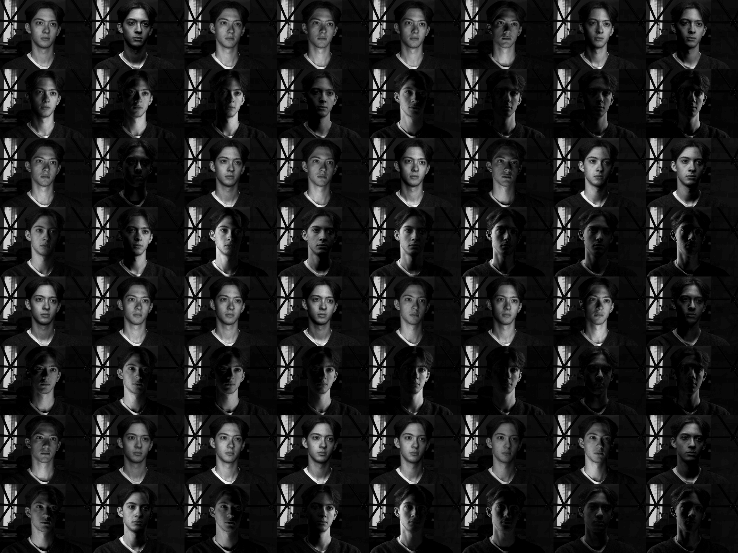
In order to remove the artifacts by unsupervised learning, we approximate the full dataset including the artificial face images by a five-dimensional subspace () using rreaper, which should be robust against the four outliers. Projecting the first four images to the recovered subspace, we removed the unwanted artifacts, see Figure 5.b and 6–7.


Note that in this example the projection corresponds to a 307 200307 200 matrix, which would require 703.125 GiB for double precision whereas the matrix-free representation only requires around 16.407 MiB since the rank of the primal variable is here bounded by seven, see Figure 8. Further, we want to mention that the primal-dual minimization algorithm for rreaper converges already after few iterations.
9 Conclusion
Convex models are usually preferable over non-convex ones due to their unique local minimum. While robust PCA models that can handle high dimensional data are usually nonconvex, a convex relaxation was proposed by the reaper model. Relying on the projector approach it is however not applicable for high dimensional data in its original form. To manage such data, we have combined primal-dual optimization techniques from convex analysis with sparse factorization techniques from the Lanczos algorithm. Moreover, we extended the model by penalizing the nuclear norm of the operator which has the advantage that the dimension of the low dimensional subspace must not be known in advance. We addressed the problem of the bias in robust PCA, but more research in this directions appears to be necessary. Further other sparsity promoting norms then the nuclear norm could be involved. Our method can be enlarged to 3D images as videos, 3D stacks of medical or material images, where tensor-free methods will come into the play. Finally, it may be interesting to couple PCA ideas with approaches from deep learning to better understand the structure of both.
Acknowledgment
The authors want to thank G. Schneck for providing the idea of the proof for Theorem 7. Funding by the German Research Foundation (DFG) within the project STE 571/16-1 and by the Austrian Science Fund (FWF) within the project P28858 is gratefully acknowledged.
References
- [1]
- [Bec17] Beck, Amir: First-Order Methods in Optimization. Philadelphia : Society for Industrial and Applied Mathematics (SIAM), Mathematical Optimization Society, 2017
- [BS15] Beck, Amir ; Sabach, Shoham: Weiszfeld’s method: Old and new results. In: Journal of Optimization Theory and Applications 164 (2015), No. 1, pp. 1–40. – ISSN 0022–3239
- [BSS16] Burger, M. ; Sawatzky, A. ; Steidl, G.: First Order Algorithms in Variational Image Processing. In: Glowinski, Roland (Ed.) ; Osher, Stanley J. (Ed.) ; Yin, Wotao (Ed.): Splitting Methods in Communication, Imaging, Science, and Engineering. Cham : Springer, 2016, pp. 345–407
- [CLMW11] Candes, Emmanuel J. ; Li, Xiaodong ; Ma, Yi ; Wright, John: Robust principal component analysis? In: Journal of the ACM 58 (2011), No. 3, pp. 11
- [CP16] Chambolle, Antonin ; Pock, Thomas: An introduction to continuous optimization for imaging. In: Acta Numerica 25 (2016), pp. 161–319
- [DZHZ06] Ding, Chris ; Zhou, Ding ; He, Xiaofeng ; Zha, Hongyuan: -PCA: rotational invariant -norm principal component analysis for robust subspace factorization. In: Proceedings of the 23rd international conference on Machine learning ACM, 2006, pp. 281–288
- [EHY95] Epstein, R. ; Hallinan, P. W. ; Yuille, A. L.: 52 eigenimages suffice: an empirical investigation of low-dimensional lighting models. In: Proceedings of the Workshop on Physics-Based Modeling in Computer Vision, 18–19 June 1995, Cambridge, USA, 1995, pp. 108–116
- [FB87] Fischler, Martin A. ; Bolles, Robert C.: Random sample consensus: a paradigm for model fitting with applications to image analysis and automated cartography. In: Readings in Computer Vision. Elsevier, 1987, pp. 726–740
- [GBK01] Georghiades, A.S. ; Belhumeur, P.N. ; Kriegman, D.J.: From few to many: illumination cone models for face recognition under variable lighting and pose. In: IEEE Trans. Pattern Anal. Mach. Intelligence 23 (2001), No. 6, pp. 643–660
- [GV13] Golub, Gene H. ; Van Loan, Charles F.: Matrix Computations. 4th edition. Baltimore : The John Hopkins University Press, 2013
- [HJ91] Horn, Roger A. ; Johnson, Charles R.: Matrix Analysis. Cambridge University Press, 1991
- [HR09] Huber, Peter J. ; Ronchetti, Elvezio M.: Robust Statistics. 2nd. Wiley, 2009
- [KK05] Ke, Qifa ; Kanade, Takeo: Robust norm factorization in the presence of outliers and missing data by alternative convex programming. In: Computer Vision and Pattern Recognition, 2005. CVPR 2005. IEEE Computer Society Conference on Vol. 1 IEEE, 2005, pp. 739–746
- [KKSZ08] Kriegel, H. P. ; Kröger, P. ; Schubert, E. ; Zimek, A.: A General Framework for Increasing the Robustness of PCA-Based Correlation Clustering Algorithms. In: Scientific and Statistical Database Management. Lecture Notes in Computer Science. 5069, 2008, pp. 418–435
- [KTV94] Kent, John T. ; Tyler, David E. ; Vard, Yahuda: A curious likelihood identity for the multivariate -distribution. In: Communications in Statistics-Simulation and Computation 23 (1994), No. 2, pp. 441–453
- [Lan50] Lanczos, Cornelius: An iteration method for the solution of the eigenvalue problem of linear differential and integral operators. In: J Res Nat Bur Standards 45 (1950), No. 4, pp. 255–282
- [LHK05] Lee, K.C. ; Ho, J. ; Kriegman, D.: Acquiring linear subspaces for face recognition under variable lighting. In: IEEE Trans. Pattern Anal. Mach. Intelligence 27 (2005), No. 5, pp. 684–698
- [LM99] Li, Chi-Kwong ; Mathias, Roy: The Lidskii-Mirsky-Wielandt theorem – additive and multiplicative versions. In: Numer Math 81 (1999), pp. 377–413
- [LM18] Lerman, Gilad ; Maunu, Tyler: An Overview of Robust Subspace Recovery. In: Proceedings of the IEEE 106 (2018), No. 8, pp. 1380–1410
- [LMTZ15] Lerman, G. ; McCoy, M. ; Tropp, J. A. ; Zhang, T.: Robust Computation of linear models by convex relaxation. In: Foundations of Computational Mathematics 15 (2015), No. 1, pp. 363–410
- [LNNS19] Lellmann, J. ; Neumayer, S. ; Nimmer, M. ; Steidl, G.: Methods for finding the offset in robust subspace fitting. In: PAMM 19 (2019), No. 1
- [LR87] Leroy, Annick M. ; Rousseeuw, Peter J.: Robust regression and outlier detection. In: Wiley Series in Probability and Mathematical Statistics (1987)
- [MT11] McCoy, Michael ; Tropp, Joel A.: Two proposals for robust PCA using semidefinite programming. In: Electronic Journal of Statistics 5 (2011), pp. 1123–1160
- [MVD97] Meng, Xiao-Li ; Van Dyk, David: The EM algorithm - an old folk-song sung to a fast new tune. In: Journal of the Royal Statistical Society: Series B (Statistical Methodology) 59 (1997), No. 3, pp. 511–567
- [MZL19] Maunu, Tyler ; Zhang, Teng ; Lerman, Gilad: A well-tempered landscape for non-convex robust subspace recovery. In: Journal of Machine Learning Research 20 (2019), No. 37, pp. 1–59
- [NNSS20] Neumayer, S. ; Nimmer, M. ; Setzer, S. ; Steidl, G.: On the rotational invariant -norm PCA. In: Linear Algebra and its Applications 587 (2020), pp. 243–270
- [NNSSar] Neumayer, Sebastian ; Nimmer, Max ; Setzer, Simon ; Steidl, Gabriele: On the Robust PCA and Weiszfeld’s Algorithm. In: Applied Mathematics & Optimization (to appear)
- [OJ78] Ostresh Jr., L. M.: On the convergence of a class of iterative methods for solving the Weber location problem. In: Operations Research 26 (1978), No. 4, pp. 597–609
- [Pea01] Pearson, K.: On Lines and Planes of Closest Fit to Systems of Points in Space. In: Philosophical Magazine 2 (1901), No. 11, pp. 559–572
- [PSH14] Podosinnikova, Anastasia ; Setzer, Simon ; Hein, Matthias: Robust PCA: Optimization of the robust reconstruction error over the Stiefel manifold. In: German Conference on Pattern Recognition Springer, 2014, pp. 121–131
- [RL05] Rousseeuw, Peter J. ; Leroy, Annick M.: Robust regression and outlier detection. Vol. 589. John Wiley & Sons, 2005
- [Roc70] Rockafellar, R. T.: Convex Analysis. Princeton University Press, 1970
- [SST12] Setzer, S. ; Steidl, G. ; Teuber, T.: On vector and matrix median computation. In: Journal of Computational and Applied Mathematics 236 (2012), No. 8, pp. 2200–2222
- [TP91] Turk, Matthew ; Pentland, Alex: Eigenfaces for Recognition. In: Journal of Cognitive Neuroscience 3 (1991), No. 1, pp. 71–86
- [Tyl87a] Tyler, David E.: A Distribution-Free -Estimator of Multivariate Scatter. In: The Annals of Statistics 15 (1987), März, No. 1, pp. 234–251
- [Tyl87b] Tyler, David E.: A distribution-free -estimator of multivariate scatter. In: The Annals of Statistics 15 (1987), No. 1, pp. 234–251
- [Wei37] Weiszfeld, E.: Sur le point pour lequel les sommes des distances de points donnés et minimum. In: Tôhoku Mathematical Journal 43 (1937), pp. 355–386
- [WS00] Wu, Kesheng ; Simon, Horst: Thick-restart Lanczos method for large symmetric eigenvalue problems. In: SIAM J Matrix Anal Appl 22 (2000), No. 2, pp. 602–616
- [XCS12] Xu, H. ; Caramanis, C. ; Sanghavi, S.: Robust Robust PCA via outlier pursuit. In: IEEE Transactions on Information Theory 58 (2012), No. 3, pp. 3047–3064