Second largest Eigenpair Statistics for Sparse Graphs
Abstract
We develop a formalism to compute the statistics of the second largest eigenpair of weighted sparse graphs with nodes, finite mean connectivity and bounded maximal degree, in cases where the top eigenpair statistics is known. The problem can be cast in terms of optimisation of a quadratic form on the sphere with a fictitious temperature, after a suitable deflation of the original matrix model. We use the cavity and replica methods to find the solution in terms of self-consistent equations for auxiliary probability density functions, which can be solved by an improved population dynamics algorithm enforcing eigenvector orthogonality on-the-fly. The analytical results are in perfect agreement with numerical diagonalisation of large (weighted) adjacency matrices, focussing on the cases of random regular and Erdős-Rényi graphs. We further analyse the case of sparse Markov transition matrices for unbiased random walks, whose second largest eigenpair describes the non-equilibrium mode with the largest relaxation time. We also show that the population dynamics algorithm with population size does not actually capture the thermodynamic limit as commonly assumed: the accuracy of the population dynamics algorithm has a strongly non-monotonic behaviour as a function of , thus implying that an optimal size must be chosen to best reproduce the results from numerical diagonalisation of graphs of finite size .
1 Introduction
The second largest eigenvalue and the associated second eigenvector of a matrix is of great significance in many areas of science, with plenty of applications. In coding theory, the Hamming distance of a binary linear code can be expressed as a function of the second largest eigenvalue of the coset graph associated to the code [1]. In biology, it has been shown in [2] that the second largest eigenvalue of cancer metabolic networks describes the speed of cancer processes. In the context of clustering methods based on the adjacency matrix of a graph, the second eigenvector encodes inter-cluster connectivity, complementing the information about intra-cluster connectivity included in the top eigenvector [3, 4]. Moreover, in Principal Component Analysis, the second eigenvector of the covariance matrix of standardised data represents the direction that accounts for the second largest source of variability within the dataset [5, 6].
The second largest eigenvalue plays a pivotal role in the study of complex systems and graph theory, representing topological features of the graphs [7]. If the spectral gap, i.e. the distance between the largest and second largest eigenvalue, is large, then the graph has good connectivity and expansion properties [8]. Therefore, many results have been derived about bounds for the second largest eigenvalue (see e.g. [9, 10]). In particular, bipartite regular graphs with very wide spectral gaps are called expanders (magnifiers if not bipartite) and have been widely studied since the seminal work of Alon [11]. To shed light on the expansion properties of regular graphs, specific bounds have been derived for their second largest eigenvalue (see e.g. [1] and [12]).
The knowledge of the spectral gap is essential for random walks on undirected graphs, which are substantially equivalent to finite time-reversible Markov chains, as pointed out by Lovasz in his survey [13]. Indeed, up to log-factors, the inverse spectral gap of the transition matrix represents the mixing rate of the Markov chain, i.e. how fast the state probability vector of a Markov chain approaches the limiting stationary distribution [14], given by the top right eigenvector of the transition matrix. The inverse of absolute value of second largest eigenvalue of the transition matrix denotes the largest relaxation time or mixing time, and the corresponding eigenvector describes the non-equilibrium mode with the slowest decay rate. The second largest eigenpair of Markov transition matrices also plays an important role in all processes that are described by means of random walks on graphs, such as out of equilibrium dynamics of glassy systems (see e.g. [15, 16]) and search algorithms such as Google PageRank [17].
In our analysis, we will be dealing with sparse symmetric random matrices, i.e. weighted adjacency matrices of undirected graphs. We focus on the case of high sparsity, i.e. when the probability of two nodes being connected is , with being the constant mean degree of nodes. In this sparse limit, numerical studies have shown that most of the eigenvectors of a random regular graph, as well as almost-eigenvectors11 1 An almost-eigenvector of a matrix with eigenvalue is a normalised vector that satisfies the eigenvector equation within some small tolerance , i.e. . [18], follow a Gaussian distribution [19], whereas Erdős-Rényi eigenvectors are localised especially for low values of . The statistics of the first eigenvector components for very sparse symmetric random matrices has been first considered in the seminal work by Kabashima and collaborators [20] and subsequently in a more systematic way in our previous work [21]. Localisation properties of eigenvectors of sparse non-Hermitian random matrices have been investigated in [44].
Following the framework developed in [21], we look at the second largest eigenpair problem as the top eigenpair problem for a deflated version of the original sparse matrix (see discussion in Section 2). We will be implementing a Statistical Mechanics formulation of the top eigenpair problem of the deflated matrix, using both the cavity (Section 3) and replica (A) methods in a unified way.
Both the replica and cavity methods from the physics of disordered systems have been employed in the realm of random matrix theory for a long time. The replica method, traditionally used in the physics of spin glasses [22], was first introduced in the context of random matrices by Edwards and Jones [23] to compute the average spectral density of random matrices defined in terms of the joint probability density function of their entries. Later on, the same approach proved useful to derive the spectral density of Erdős-Rényi adjacency matrices as the solution of an intractable integral equation in the seminal paper of Bray and Rodgers [24]. Later, approximation schemes such as the single defect approximation (SDA) and the effective medium approximation (EMA) [25, 26] were developed. An exact alternative approach was introduced in [27]: starting from Bray-Rodgers replica-symmetric setup [24], the functional order parameters of the theory are expressed as continuous superpositions of Gaussians with fluctuating variances, as suggested by earlier solutions of models for finitely coordinated harmonically coupled systems [28]. This formulation gives rise to non-linear integral equations for the probability densities of such variances, which can be efficiently solved by a population dynamics algorithm. We will follow a similar approach in A.
The cavity method [29] has been employed in the study of disordered systems and sparse random matrices as a more direct alternative to replicas. It is exact for highly sparse tree structures [30]. As shown in [31], one of the advantages of the cavity method is that it provides the spectral density for very large single instances of sparse random graphs. Both methods, known to lead to the same results for the spectral density [32], recover the Kesten-McKay law for the spectra of random regular graphs [33, 34], the Marčenko-Pastur law and the Wigner’s semicircle law respectively for sparse covariance matrices, and for Erdős-Rényi adjacency matrices in the large limit [27, 31]. Likewise, the spectral density of sparse Markov matrices [35, 36], graphs with modular [37] and small-world [38] structure, and with topological constraints [39] have been obtained. Also, the spectral density in the complex plane of sparse non-Hermitian matrices has been considered in [40, 41, 42, 43].
As in [21], we will provide a cavity single-instance derivation for our problem. Generalising the single-instance results in the thermodynamic limit, we will show that even for the second eigenpair problem the cavity method leads to the same stochastic recursions obtained from the replica treatment. The crucial difference between the present work and [21] is the presence of the orthogonality condition between the top and second eigenvectors in the set of final recursion equations. The population dynamics algorithm employed to solve these recursions, complemented by a wise implementation of the orthogonality constraint, allows us to characterise the distributions of the cavity fields in the thermodynamic limit, and to disentangle the individual contributions of different degrees to the second eigenvector’s entries.
The plan of the paper is as follows. In Section 2, we will formulate the problem in terms of deflation and provide the main starting point. In Section 3, we will describe the cavity approach to the problem, first for the single instance case, and then in the thermodynamic limit, highlighting the role of the orthogonality constraint (in 3.3.1). To complement the cavity results, we offer an equivalent replica treatment in A. In Section 4 we focus on the case of the random regular graph: we analytically show how the solution for the top eigenpair of the deflated adjacency matrix gets modified as the deflation parameter is changed. In Section 5, we specialise our results to the case of Markov transition matrices representing random walks on graphs. In Section 6, we provide the details of the population dynamics algorithm, focussing on how the extra orthogonality constraint is implemented. We also provide convincing evidence that – at odds with what is commonly believed – the algorithm with finite population size does not actually capture the thermodynamic limit , in that there is a non-trivial relation between the size of the adjacency matrix being diagonalised, and the size of the population one should ideally use to numerically compute its spectral properties. More precisely, the accuracy – measured with different metrics – with which the population dynamics algorithm reproduces numerical diagonalisation of matrices (graphs) of size has a strongly non-monotonic behaviour as a function of , thus implying that an optimal size must be chosen to best reproduce the diagonalisation results. Finally, in Section 7 we offer a summary of results.
2 Formulation of the problem
We consider a real sparse symmetric random matrix and assume that its top eigenpair is known. We define a deflated matrix by
| (1) |
where represents the deflation parameter. The top eigenvector of is normalised such that .22 2 The same normalisation convention applies to all the other eigenvectors of , with . In what follows, the vector will be also referred to as the probe eigenvector. The dense matrix represents the projector onto the top eigenspace of the original matrix . The are the i.i.d. entries of the original sparse symmetric random matrix . They are defined in terms of the connectivity matrix , i.e. the adjacency matrix of the underlying graph, and the random variables encoding bond weights. Within our formalism, we are able to handle any kind of highly sparse degree connectivity - where the mean node degree is a finite constant that does not scale with (entailing as ). We will typically consider bounded degree distributions: a candidate of interest can be represented by a bounded Poisson distribution
| (2) |
with the mean degree and for normalisation. The bond weights will be i.i.d. random variables drawn from a parent pdf with bounded support. This setting is sufficient to ensure that the largest eigenvalue of will remain of for .
The spectral theorem ensures that can be diagonalised via an orthonormal basis of eigenvectors with corresponding real eigenvalues (),
| (3) |
for each eigenpair , where to simplify notation we have omitted the -dependence. Assume that there is no eigenvalue degeneracy, and that they are sorted , and the same holds for the eigenvalues () of the original matrix .
For any value of , the matrices and share the same set of eigenvectors (see Section 3.3.2 in [45]). The range of the deflation parameter is , where the boundaries of this range correspond respectively to no deflation () and full deflation ().
- •
When the value of is smaller than the spectral gap , the top eigenvalue of is given by with corresponding eigenvector . Indeed:
(4) with . We recall that .
- •
Conversely, when then the second largest eigenvalue of , , and the corresponding eigenvector become the top eigenpair of the matrix . Indeed, following (4), the top eigenvector of , , is still an eigenvector of related to the eigenvalue but now . Clearly,
(5) in view of the orthogonality between and .
- •
In particular, when , i.e. for full deflation33 3 In the thermodynamic limit, the value of such that full deflation is achieved is actually the average largest eigenvalue of the matrix ., the top eigenvector of , , is still an eigenvector of , but corresponding to a zero eigenvalue. Indeed,
(6) - •
All other eigenpairs are unchanged.
By setting up a formalism based on the statistical mechanics of disordered systems, we aim to find the average (or typical) value of the second largest eigenvalue of , and the density of the corresponding second largest eigenvector’s components, . The second eigenpair statistics of the matrix is obtained by finding the top eigenpair of the deflated matrix when . Thus, in order to obtain the desired quantities, we analyse the average largest eigenvalue and the density of the top eigenvector’s components, of the deflated matrix , where the average is taken over the distribution of the matrix .
We provide:
- •
the second largest eigenpair statistics and of the matrix , i.e. the solution corresponding to the maximum deflation for , in the case of a generic connectivity with bounded maximum degree, found via the cavity method (Section 3). We also offer an equivalent replica derivation for the same problem (A). In this general case, the solution is available via population dynamics simulations (Section 6);
- •
an explicit analytical solution for and in the specific case of the adjacency matrix of a random regular graph (RRG), showing that the solution requires that the deflation parameter exceed the spectral gap (Section 4);
- •
the second largest eigenpair statistics of the unbiased random walk Markov transition matrix. In this case, the deflation parameter is set precisely to 1, i.e. equal to the largest eigenvalue of the Markov transition matrix. Also in this case, an analytical description is provided for the RRG connectivity case (Section 5).
The equations (55), (56), (57) and (58) found below within the cavity framework (see Section 3.3.1) represent the solution of the second largest eigenpair problem in the thermodynamic limit, and constitute the main result of this paper. We notice that they are completely equivalent to the equations (180), (181), (182) and (183) found within the replica framework (see A.2).
We will follow the same protocol used in [21]. Focussing on the matrix , the problem can be formulated as the optimisation of a quadratic function , according to which is the vector normalised to that realises the condition
| (7) |
as dictated by the Courant-Fischer definition of eigenvectors. The round brackets indicate the dot product between vectors in . It is easy to show that is bounded
| (8) |
and attains its minimum when computed on the top eigenvector.
For a fixed matrix , the minimum in (7) can be computed by introducing a fictitious canonical ensemble of -dimensional vectors at inverse temperature , whose Gibbs-Boltzmann distribution reads
| (9) |
where the delta function enforces normalisation. Clearly, in the low temperature limit , only one “state” remains populated, which corresponds to , the top eigenvector of the matrix .
3 Full deflation: cavity method
In this section, we present the cavity derivation of the single instance equation for the second largest eigenpair problem. The formalism shown here differs from that presented in [21]: here we analyse the partition function of the Boltzmann distribution (9), rather than a soft-constrained version of it. This allows us to include hard constraints within the cavity framework. The equations expressing the solution can be easily generalised to the thermodynamic limit case, reproducing the same equations that will be found by the replica formalism in A, which constitute the main results of this work.
3.1 Top eigenpair of a single instance: generic deflation case
Given a single instance matrix , its largest eigenvalue can be defined as
| (10) |
The partition function explicitly reads
| (11) |
The square in the exponent can be written as
| (12) |
with the identification
| (13) |
The definition of the order parameter is enforced via the integral identity
| (14) |
By also employing a Fourier representation of the Dirac delta enforcing the normalisation constraint and including all the pre-factors in , the partition function becomes
| (15) |
where
| (16) |
defines the action with
| (17) |
The matrix is related to the resolvent of . It has the same eigenvectors as , thus using the spectral theorem it can be expressed as
| (18) |
where the are the eigenvalues of and the are their corresponding eigenvectors. Notice that the are normalised such that . On the other hand, the vector appearing in the exponent of is the top eigenvector of , , normalised such that . Therefore,
| (19) |
entailing that
| (20) |
In turn, the action (16) becomes
| (21) |
Taking into account (21), Eq. (15) can be evaluated with a saddle-point approximation for large . The stationarity of (21) w.r.t. to , and implies that
| (22) | ||||
| (23) | ||||
| (24) |
| (25) |
Two cases can be distinguished, depending on the value of .
- 1.
Assuming , Eq. (25) yields , while from (22) it follows that . Using these results to express the action , one finds
(26) entailing for the largest eigenvalue defined in (10)
(27) As stated in Section 2, this is the top eigenvalue of when . Indeed, the value indicates that the the probe eigenvector and the top eigenvector of corresponding to coincide. Thus, when the deflation parameter is smaller that the spectral gap , there is no need to use the cavity method to obtain the top eigenpair of the deflated matrix, which is simply given by .
- 2.
Assuming , it follows from (24) that . Thus the action reduces to
(28) The case provides the top eigenvalue of the deflated matrix in the case , including the case of full deflation . Therefore, represents the orthogonality condition between the solution and the probe eigenvector . In this scenario, the top eigenvalue of the matrix is the second largest eigenvalue of the original matrix , viz.
(29) However, the stationarity conditions (22),(23) and (24) do not provide the actual (real) value , nor the components of the corresponding eigenvector .
To sum up, the top eigenvalue of the deflated matrix is always given by the value , regardless the value of . However, for this value needs to be determined via the cavity method, as detailed in the next subsection.
3.2 Cavity derivation for a single instance in case of full deflation
We focus on the case of full deflation . This choice is not restrictive, since the solution does not depend on , for any . As shown before, in the range one has . However, for the time being we proceed with a generic . Its actual value will be made explicit in the final result.
One looks at (15), without performing explicitly the integration in (17). Considering the stationarity of the action w.r.t , and , the following conditions hold,
| (30) | ||||
| (31) | ||||
| (32) |
where the starred quantities indicate the saddle-point values of the parameters. The angular brackets indicate averaging w.r.t. the distribution
| (33) |
By looking at the saddle point condition (30), in what follows we can identify (omitting the star for brevity) and define , such that (33) becomes
| (34) |
The components are found in the limit by the cavity method applied to the distribution (34) 44 4 It can be noticed that the distribution (34) is substantially equivalent to the grand-canonical distribution (Eq. (7) in [21]) which we adopt as the starting point of the cavity treatment in [21].. Here we will follow the protocol detailed in Section 3.1 of [21], reporting the key steps to make this paper self-contained.
By making a tree-like assumption on the structure of the highly sparse graph encoded in the original matrix that we deflate, the marginal pdf w.r.t. a certain component is given by
| (35) |
where denotes the immediate neighbourhood of . The factorisation over the neighbouring nodes of is due to the fact that in a tree-like structure the nodes are connected with each other only through . The distribution is called marginal cavity distribution: it is the distribution of the components defined on the neighbouring nodes of , in the network in which has been removed.
In the same way (see for instance Eq. (11) in [21]), for any the cavity marginal pdf satisfies the self-consistent equation
| (36) |
where indicates the set of neighbours of the node with the exclusion of .
A Gaussian ansatz provides the solution to the self consistent equation, viz.
| (37) |
where the parameters and are called cavity fields. By inserting the ansatz in (36) and performing the Gaussian integrals, the set of self-consistent equations represented by (36) translates into a set of recursions for the cavity fields,
| (38) |
| (39) |
Likewise, by means of (37), the marginal distribution can be written as
| (40) |
where
| (41) |
| (42) |
Using the cavity factorisation in (40) to express (34), we eventually obtain
| (43) |
In the limit,
| (44) |
entailing that the components of the top eigenvector of the fully deflated matrix , representing the ground state of the system with Boltzmann distribution (9), are given by the ratios . The and the are determined respectively by Eq. (41) and (42). Because of the full deflation, also represents the second largest eigenvector of the original matrix .
In terms of Eq. (44), the conditions (31) and (32) read
| (45) | ||||
| (46) |
At this point, we recall that for any (in particular ), we have . Therefore must be considered in Eq. (39) and (42), and the condition (45) becomes
| (47) |
As anticipated in Section 3.1, Eq. (47) expresses the orthogonality condition between and . The components and in (47) are naturally referring to the same node with degree of the network represented by .
To summarise, in the single instance full-deflation case the solution is given by the cavity recursions (38) and (39) along with the normalisation condition (46) and the orthogonality constraint (47). The value represents the second largest eigenvalue of the matrix (i.e. the top eigenvalue of the deflated matrix ), with corresponding eigenvalue whose components are defined in Eq. (44). According to the same mechanism explained in Appendix A of [21], it is the only value that satisfies the normalisation condition (46).
3.3 Cavity method: thermodynamic limit
Following the reasoning of Section 3.2 in [21], in the limit we can consider the joint probability density of the cavity fields and taking values around respectively and ,
| (48) |
where , and the average is taken over independent realisations of the bond weights . Here, is the distribution of the top eigenvector’s component of conditioned to the degree . The distribution represents the probability that a randomly chosen link points to a node of degree and , and appears in (48) as cavity fields are related to links. Eq. (48) generalises in the thermodynamic limit the recursions (38) and (39) in the case of full deflation ().
By using the law of large numbers, in the thermodynamic limit the normalisation condition (46) reads
| (49) |
whereas the orthogonality constraint (45) becomes
| (50) |
Similarly, the distribution of the top eigenvector’s components of the fully deflated matrix , i.e. the second largest eigenvector of , is obtained in terms of averages w.r.t. the distribution as
| (51) |
We notice that in the equations (49), (50) and (51), the degree distribution naturally crops up, as they encode properties related to nodes, rather than links. Moreover, Eq. (29) generalises to the thermodynamic limit case, as
| (52) |
for any . We anticipate that the latter result is equivalent to the average second largest eigenvalue explicitly found by the replica approach in Eq. (168) in A. Finally, we remark that Eq. (27) generalises at the ensemble level too, entailing the condition
| (53) |
which is valid when .
3.3.1 Cavity method: the orthogonality condition
The condition , valid whenever exceeds the spectral gap, holds at the ensemble level as well. Indeed, when considering , Eq. (50) encodes the orthogonality-on-average condition between the probe eigenvector and the top eigenvector of the deflated matrix , corresponding to the second largest eigenvector of the original matrix . The interpretation of Eq. (50) for is made clearer by simply considering the average orthogonality condition between and , viz.
| (54) |
where indicates the joint probability density of the first and second largest eigenvector’s components of , and the conditional pdf is obtained from (51) erasing the -integration and the -sum. The conditional pdf is given by omitting the -sum in the expression for the density of the top eigenvector components (60). Comparing Eq. (54) with (50) for , it follows that they are equivalent.
Taking into account the average orthogonality condition , the equations (48), (49), (50), (51) and (52) simplify to
| (55) | ||||
| (56) | ||||
| (57) | ||||
| (58) | ||||
| (59) |
where we have used the shorthand .
Enforcing the orthogonality condition given by (57) is crucial to find the correct solution. The conditional pdf appearing in (57) is given by omitting the -sum in the expression for the density of the top eigenvector components (see Eq. (111) in [21]), reported here
| (60) |
where indicates the distribution of cavity fields of type and for the top eigenpair problem55 5 In the context of the top eigenpair problem, the cavity field of type has the role of an inverse cavity variance (similarly to for the second largest eigenpair problem), whereas represents a cavity bias (similarly to here). See Section 3 in [21].. The integration w.r.t. the conditional distribution in (57) generalises to the thermodynamic limit the fact that both the components and in (47) refer to the same node with degree . Indeed, by comparing (60) with (58) and (57), we notice that the components of are still coupled to those of in (57) through their structure, as they both refer to the same degree (see Section 6 for more details). The replica derivation in A provides an independent proof of this result.
Therefore, in order to enforce the constraint (57) correctly, we need to impose strict orthogonality on-the-fly, i.e. while the components of the top eigenvector and the components of the second largest eigenvector are being evaluated at the same time by averaging w.r.t. respectively and , as prescribed by (60) and (55). The way strict orthogonality is imposed is via a correction to the components of : the details of this procedure and the corresponding algorithm are given in Section 6. We remark that the condition holds whenever exceeds the spectral gap.
To summarise, the equations (55), (56), (57), (58) and (59) represent the solution of the second largest eigenpair problem in the thermodynamic limit and constitute the main result of this paper. This set of equations must be generally solved by a population dynamics algorithm, as detailed in Section 6. It is completely equivalent to the equations (180), (181), (182), (184) and (183), respectively, found within the replica framework (See A.2).
Figure 1 shows the numerical results in the case of an Erdős-Rényi (ER) adjacency matrix with and . We find , within a 2% error w.r.t. the value obtained by extrapolation from the direct diagonalisation data. The bottom right panel of Figure 1 refers instead to the case of ER weighted adjacency matrix with and . We consider the case of uniform distribution of bond weights, for . In this case, we find , within a 2.5% error w.r.t. the reference value obtained by extrapolation from the direct diagonalisation data. In the plot, we compare the pdf of second largest eigenvector’s components obtained via population dynamics with results from the direct diagonalisation of matrices of size .
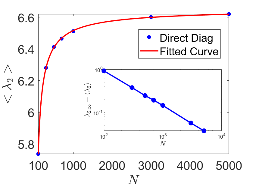
Figure 2 compares the theoretical results for the pdf of the second largest eigenvector’s components with results of direct numerical diagonalisation for adjacency matrices of ER graphs with and . In this case, we find , within a error w.r.t. the value obtained by extrapolation from the direct diagonalisation data. We observe that there are finite size effects in the distribution of eigenvector components that are significantly stronger than those observed in the eigenvalue problem. The bottom panel of figure 2 shows the average second largest eigenvalue as a function of the matrix size , obtained via direct diagonalisation of adjacency matrices of ER graphs with and . The data are fitted by a power law curve , with for this type of network. The inset shows the plot of against in log scale, confirming that the power law exponent is positive. The power law convergence is a common behaviour found in all ensembles analysed in this paper, though the value of the exponent depends on details of the systems.


4 Random regular graphs
For non-weighted adjacency matrices of RRGs, the degree distribution is simply , and the bond weights distribution is trivially , resulting in a constant probe top eigenvector , i.e. . The largest eigenvalue is non-random and pinned to the value . The spectral density is given by the Kesten-McKay distribution (See Figure 3),
| (61) |
In this section we look at the behaviour of the solution for a generic value of the deflation parameter in the range . Therefore, the value of is in principle non-zero. We remark that holds surely in the case of full deflation, as in Section 3 (and A). For a general value of the deflation parameter , the equation (48) for , along with the conditions (49) and (50) become respectively
| (62) | ||||
| (63) | ||||
| (64) |
and the density of the top eigenvector’s components of the deflated matrix (51) is given for general by
| (65) |
We will show that the solution of the self-consistency equation (62) along with (63), (64) and (65) crucially depends on the value of the deflation parameter . We recall here that the range of is , where the boundaries of this range correspond respectively to no deflation () and full deflation ().
We anticipate that in the outer regime (see Figure 3), the probe eigenvector , i.e. the top eigenvector of the original matrix , is also the top eigenvector of the deflated matrix , with corresponding largest eigenvalue lying outside the bulk of the Kesten-McKay spectrum [33, 34]. Conversely, in the bulk regime i.e. when , the top eigenvector’s components density is a standard normal distribution, with corresponding largest eigenvalue . The probe all-one eigenvector is still an eigenvector of but refers to an eigenvalue . In other words, we show that the second largest eigenpair of the RRG adjacency matrix is given by and . Figure 3 explains graphically the outer and bulk regimes.

The abrupt change of the solution (from constant to normally distributed when hits the value ) reflects the fact that the usual peaked ansatz for the RRG case (see [21]) is not valid in the bulk regime . Therefore, in order to solve the self-consistency equation (62), we choose a “mixed” ansatz of the form
| (66) |
for real and .
We further show that in the range , the solution reduces to a peaked ansatz, i.e. - just like in the case of the largest eigenpair of the original matrix - whereas in the range , the variance must be finite.
Indeed, by inserting (66) into (62) and performing the r.h.s. integrals, we find
| (67) |
Comparing (67) with the ansatz (66), we find that the following relations must be satisfied
| (68) | ||||
| (69) | ||||
| (70) |
From the last condition (70), we can infer that if , then , i.e. a finite variance of the distribution of components pins to a specific value. Only if , then can assume values other than , according to Eq. (68).
Inserting the ansatz (66) in the normalisation condition (63) and in the condition (64), we find two extra conditions to fix respectively and ,
| (71) | ||||
| (72) |
By combining (68), (69) and (72), we find an expression for in terms of and ,
| (73) |
which in turn can be inserted into Eq. (69) to give
| (74) |
Comparing eq. (68) rewritten as
| (75) |
with a slight rewriting of the condition that the expression in the round brackets of (74) be zero, viz.
| (76) |
we notice that (75) and (76) can be compatible only if the coefficient of is the same, entailing . Moreover, by solving (76) for we also find the explicit dependence of on . Indeed, we get
| (77) |
By imposing that the radicand be positive in order to get a real solution, we find that eq. (77) yields a -dependent real solution only for . Only in this regime, can assume values other than , entailing from (70) a peaked solution for .66 6 We remark that in this regime a finite variance solution for that pins to is still possible, but yields a higher ground state free energy than the peaked solution. Indeed, . See Sections 4.1 and 4.3.
Conversely, for any , Eq. (77) would produce a -dependent complex solution , which is not acceptable for this problem (recall that and must be real), thus implying
| (78) |
4.1 RRG-deflated top eigenvalue: outer regime
| (79) |
When solving (79), we must discard the other possible solution , since it would not satisfy the normalisation constraint (63).
Equipped with this information and also taking into account (66), (76) and the identity , which follows from (73), we find for the average of the largest eigenvalue of the formula
| (80) |
which is exactly equal to as expected (see (53)). Details of the replica computation that leads to this result can be found in B.
Therefore, the deflation with a parameter in the regime has the effect of decreasing the top eigenvalue of the original RRG adjacency matrix by a quantity , as long as it lies outside the spectral bulk of the Kesten-McKay distribution. This confirms the mechanism explained in Section 2. In the next subsection, we will show that the corresponding eigenvector is still the top eigenvector of .
4.2 RRG-deflated density of top eigenvector components: outer regime
As found at the beginning of this Section, within the range , the ansatz for is delta-peaked, since . We show that a peaked ansatz of this sort corresponds to the top eigenvector of the matrix being all-ones: this means that for the top eigenvector of is exactly the probe eigenvector .
Indeed, by inserting the ansatz (66) in (65) and taking into account (76) and (79), we find
| (81) |
but, from (79),
| (82) |
implying
| (83) |
where the choice of the “” sign solution is not restrictive.
In conclusion, as long as the largest eigenvalue of the deflated matrix lies outside the spectral bulk (i.e. for ), the corresponding top eigenvector is equal to the probe eigenvector , i.e. the top eigenvector of .
4.3 RRG top eigenvalue: bulk regime
In this range, we have shown in (78) that the variance is positive, giving rise to a mixed “delta-Gaussian” ansatz for . The parameter being positive implies that must be pinned to the value . From (68), it follows that . The values of and are determined by the normalisation (63) and orthogonality (64) conditions. Indeed, the change in the ansatz corresponds to a change in the structure of the largest eigenvector of . As shown in Section 3.3, the orthogonality condition reads
| (84) |
where is the conditional distribution of the probe eigenvector’s entries and (65) has been used. Comparing (84) with (64) we infer that . Moreover, inserting in (71) and (72), we can respectively infer that
| (85) | ||||
| (86) |
Equipped with this information and also by taking into account (66), we find that the average of the largest eigenvalue of is
| (87) |
corresponding to the upper edge of the Kesten-McKay distribution, and once again exactly equal to (see (59)). Also in this case, the details of the replica calculation are in B.
As expected, the eigenvalue does not depend on the normalisation of the corresponding eigenvector, encoded in . Since this result holds for any in , including the case of full deflation when and the first eigenmode of the original matrix is associated to a zero eigenvalue, we conclude that the average second largest eigenvalue of the matrix is
| (88) |
Also in this case, we find agreement with the general deflation framework described in Section 2.
4.4 RRG density of top eigenvector components: bulk regime
In this range of values for , we show that the “delta-Gaussian” ansatz for leads to a Gaussian-distributed top eigenvector of the matrix . Since this result is valid also in case of full deflation, i.e. , we can conclude that the eigenvector corresponding to the second largest eigenvalue of a random regular graph adjacency matrix is normally distributed77 7 We remark that our method cannot provide the eigenvector statistic for . Indeed, for this specific value of , the probe eigenvector is forced to correspond to the eigenvalue , which retains its own eigenvector, thus artificially creating a degeneracy. Our method is based on the assumption of non-degeneracy of eigenvalues, so we are not able to give a result about eigenvectors in this marginal case.. We then identify in a transition point for the structure of the distribution of the top eigenvector’s components of , at which the parameter changes discontinuously from to .
We now evaluate the density of the top eigenvector components in the range . Inserting the ansatz (66) in (65) and taking into account (78), (84), (85) and (86), we find
| (89) |
We remark that this analytical result is in excellent agreement with the statistics of the second largest eigenvector components of the RRG adjacency matrices found by population dynamics, as shown in Figure 4. Moreover, it is compatible with previous known results about eigenvectors of random regular graphs [19, 18].

5 Sparse random Markov transition matrices
In this section, we apply the deflation formalism to an ensemble of transition matrices for discrete Markov chains in a -dimensional state space, in order to characterise the statistics of the second largest eigenpair. This kind of Markov chain represents a random walk on a graph. We remark here that the second largest eigenpair encodes non-equilibrium properties of a Markov process. Indeed, the inverse of the (absolute value) of the second largest eigenvalue represents the slowest relaxation time, whereas the associated second eigenvector is the non-equilibrium mode with the largest relaxation time.
We will then employ a full deflation, by setting . The evolution equation for the Markov chain states probability vector at time , , is given in terms of the matrix by
| (90) |
The transition matrix is such that and . For an irreducible chain, the top right eigenvector of the matrix corresponding to the Perron-Frobenius eigenvalue represents the unique equilibrium distribution, i.e. . The matrix is in general not symmetric. However, if the Markov process satisfies a detailed balance condition, i.e. , it can be symmetrised via a similarity transformation, yielding
| (91) |
The symmetrised matrix and its deflated version will be the target of our analysis: even though is not itself a Markov matrix since the columns normalisation constraint is lost, in view of the detailed balance condition has the same (real) spectrum as , and its top eigenvector is given in terms of the top right eigenvector of , , as
| (92) |
It is actually well-known that the relation between the eigenvectors of and those of holds in general and is not limited to the case of the top one.
We will consider the case of an unbiased random walk: the matrix is then defined as
| (93) |
where represents the connectivity matrix and is the degree of node . In this case, the top right eigenvector of is proportional to the vector expressing the degree sequence: for our purposes, we choose the inverse of the mean degree as proportionality constant, i.e. . The symmetrised matrix is expressed as
with its top eigenvector being . Thus, we have
| (94) |
where is the degree distribution of the connectivity matrix .
In order to avoid isolated nodes and isolated clusters of nodes, we consider degree distributions with and finite mean degree88 8 A suitable candidate could be a shifted Poissonian degree distribution with , i.e. (95) with mean degree . . We will provide a treatment for a generic distribution with the aforementioned properties and the analytical solution for the random regular connectivity case with degree distribution .
5.1 Second largest eigenpair of Markov transition matrices
We focus on the fully deflated symmetrised version of the Markov matrix , that is
| (96) |
where and represents the top eigenvector of , normalised to , i.e. . Here, represents the mean degree, . Our aim is to find the typical largest eigenvalue of , which corresponds to the typical second largest eigenvalue of . In the next subsection, we will characterise the distribution of the top eigenvector of , equivalent to the second eigenvector of .
We follow the same formalism illustrated in Section 3.3. An alternative replica derivation can be found in C. Here, we will just report the final equations, corresponding to (55) along with (56), (57) and (59). By taking into account (94) and the existence of , we find
| (97) | ||||
| (98) | ||||
| (99) | ||||
| (100) |
We remark that in the Markov case a bounded largest degree is not strictly necessary as the spectrum is always bounded. However, we will consider a for practical purposes. The self-consistency equation (97) along with the normalisation condition (98) and the orthogonality constraint (99) is solved by a population dynamics algorithm (See Section 6). The RRG connectivity case is analytically tractable, as shown in Section 5.2.
In analogy to Eq.(58), the density of the top eigenvector’s component of the matrix , corresponding to the second largest eigenvector of , is given by
| (101) |
where satisfies the self-consistency equation (97), supplemented by the normalisation condition (98) and the orthogonality condition (99).
Figure 5 compares the pdf of the second largest eigenvector’s components obtained via population dynamics with results obtained via direct diagonalisation, for the unbiased random walk Markov matrix case with shifted Poisson degree distribution (). We study both a low (, left panel) and a high (, right panel) connectivity case. In the case with , we find , within a 0.7% error w.r.t. the value obtained by extrapolation from the direct diagonalisation data. In the case with , we find , within a 0.1% error w.r.t. the value obtained by extrapolation from the direct diagonalisation data. As a reference point, the average value of the second largest eigenvalue in the RRG case with the same is . We notice that the agreement near the peak of the distribution is slightly worse for the low connectivity case: this is in agreement with the finding that finite-size effects are generally more pronounced for lower (see also discussion in section 6.4).


5.2 Unbiased random walk on a RRG: second largest eigenpair statistics
For a random regular graph, for which , we note that the matrix reduces to
| (102) |
implying that all results about the RRG adjacency matrix case stated in Sections 4.3 and 4.4 carry over to this case too, but with all eigenvalues rescaled by . As expected, , and the second largest eigenvalue corresponding to a -distributed eigenvector is . The spectral gap for this kind of Markov matrices as a function of is then .
6 Population Dynamics
6.1 The orthogonality challenge
With the exception of the unweighted adjacency matrix of a RRG, Eq. (55) – supplemented with the conditions (56) and (57) – must be generally solved via a Population Dynamics algorithm, a Monte Carlo technique deeply rooted in the statistical mechanics of spin glasses [47, 48].
The algorithm we use bears some similarity with the one employed in [21]. Here, we will highlight the main differences that stem from the presence of the orthogonality condition (57). We recall that the Eqs. (55), (56) and (57) refer to the case of full deflation, where we look at the top eigenpair of the deflated matrix (the second largest eigenpair of the matrix ).
Some observations are in order before sketching the algorithm. As we stated in [21], within the population dynamics algorithm the definition of the variables in Eq. (55) is effectively converted into a stochastic linear update of values. Its stability can only be achieved for . For any , the variables of type will shrink to zero, whereas for they will explode in norm. In our scenario, where we consider , the recursion is thus a priori unstable, unless it is otherwise constrained. Therefore, if unconstrained, the population will never spontaneously evolve towards a stable regime, which would at the same time satisfy the conditions (56) and (57).
As anticipated in Section 3.3, this observation entails that the orthogonality condition (57) must be strictly enforced on-the-fly – by imposing a correction to the fields , which once again have no fixed scale given by their update equation. Enforcing the constraint (57) is equivalent to looking for a self-consistent solution of (55) in a smaller, constrained space. Only once the condition (57) has been enforced, a new stable non-trivial fixed point arises, and the behaviour of the -variables is similar to that in the top eigenvector case: for any value , the variables under iteration of the modified population dynamics algorithm shrink to zero, whereas for they will explode in norm. Hence, Eq. (55) – taken together with the condition (57) – admits a stable, hence normalisable solution, such that Eq. (56) is naturally satisfied only for : after the orthogonality correction has been enforced, the procedure we follow is then exactly identical to that used in [21].
6.2 The algorithm
Taking into account the observations made in section 6.1, we briefly sketch the algorithm in the case of full deflation.
Two pairs of (coupled) populations with members each and are randomly initialised, taking into account that both and must be larger than , the upper edge of the support of the bond pdf . We typically choose or larger. In what follows, the parameter is the candidate second largest eigenvalue of , whereas is the average top largest eigenvalue of . The first population is employed to solve the top eigenpair problem, and the other to solve the second eigenpair problem; the latter is constrained by results of the former due to the orthogonality constraint.
We therefore first run a short population dynamics simulation following Section 6 in [21] involving only the population to find the solution for the first eigenpair problem and the value . This first simulation acts as an equilibration phase for the fields contributing to the largest eigenpair. Then, for any suitable value of , the following steps are iterated until stable populations are obtained:
- 1.
Generate a random , where
- 2.
Generate i.i.d. random variables from the bond weights pdf
- 3.
Select pairs and from both populations at random, where the set of population indices for the two randomly selected samples is the same for both samples; compute
(103) (104) (105) (106) and replace two randomly selected pairs and where with the pairs and .
- 4.
Compute the components of the top eigenvector and the candidate second largest eigenvector . In order to create a sample estimate of the eigenvectors statistics corresponding to the two top eigenvalues, we initialise two empty vectors, respectively and of size , where (typically if ). The square brackets indicate the integer part. Then for any :
- (a)
Generate
- (b)
Generate i.i.d. random variables from the weights pdf
- (c)
Randomly select a subset of indices from the population indices between and . This subset is denoted by . Then, for any select pairs and from both populations; compute
(107) (108) Each set of population indices labelled by contributes uniquely to a single component of the vectors and . There is a unique matching between each set of population indices and each component (see scheme in Figure 6): in other words, each group of pairs and takes part in the definition of just one component , respectively and . Each set of population indices corresponding to a specific component is then saved, along with the set of weights .
- (a)
- 5.
Compute , where indicates the dot product. In order to enforce the condition , for any component apply the correction
(109) In view of the rigid connection between the population indices labelling the fields and every specific component of and , the orthogonalisation in (109) is practically achieved by correcting each field participating in the definition of every specific component . The values of the indices here are those saved in each subset in step (iv)(c), along with the corresponding weights . For any and for any contributing to the single component of both and we have
(110) where is exactly the “degree” drawn from in step (iv)(a) and used to build each component in step (iv)(c).
- 6.
Return to (i).
A sweep is completed when all the pairs and have been updated at least once according to the steps above. The update of the pairs is stable, thanks to the prior equilibration phase. The convergence is assessed by looking only at the first moments of the two vectors formed by the samples of the pairs . The parameter is varied according to the behaviour illustrated in Section 6.1: starting from an initial “large” value , it is then progressively decreased until a non trivial distribution for the is achieved, in correspondence of the value . Indeed, we observe that for any , the shrink to zero, whereas for any , they blow up in norm.
Some comments are in order:
- •
the condition expressed in (109) is a Gram-Schmidt orthogonalisation, taking place after every microscopic update of the fields;
- •
the correction does not take place for components related to , as both and are zero;
- •
in step (iv)(c), we can clearly see that the components and are coupled through their degree and the set of bond weights, as anticipated in Section 3.3. Indeed, for any , the i.i.d. realisations of the weights and the “local neighbourhood” that we dynamically create at every step (c) must be exactly the same for both and . In other words, both and must have the same update history.

6.3 Potential for simplifications in special cases
The steps (iv) and (v) of the algorithm are computationally heavy. We are able in some cases to simplify them.
- •
For adjacency matrices of RRGs, where the variables and are constant, the correction (109) translates to forcing the mean of the to be zero after every update. Both steps (iv)-(v) are then replaced by
(111) where indicates the sample mean of the population.
- •
In the ER case (both weighted and non-weighted), we take advantage of the fact that in the thermodynamic limit there is no statistical distinction between the cavity fields and (respectively and ) and the denominator and numerator in (108), (respectively in (107)), even in presence of the truncation of the Poissonian degree distribution11 1 Provided that the largest degree is reasonably large. The only difference between the distribution and the distribution of the denominator and numerator of (58) can be observed because of the contribution coming from the largest degree, whose probability to occur is negligible.. Hence, we can consider just one couple of fields per species to represent a component, so we identify =. Steps (iv) and (v) are then replaced by
- 4.
Compute eigenvectors and as
(112) (113) - 5.
Compute the correction as
(114)
- 4.
6.4 Population dynamics algorithm describes finite-size systems.
When no simplification can be used, as in the case of Markov matrices, the population dynamics algorithm can be relatively slow, due to the number of nested updates it requires. In these cases, we have therefore been often forced to consider a population size smaller than the values we would have typically wished ( or more).
However, what may appear as a limitation at first sight turned out to be a blessing, in that it made us aware of an interesting interplay between the size of the population dynamics, and the size of the graph whose spectral properties were to be reproduced.
Indeed, we have collected convincing evidence that population dynamics at finite does not really capture the thermodynamic limit : for a given graph size , there is an optimal size of the population that best captures the spectral properties of that finite-size graph, and the degree of agreement between “theory” and numerical diagonalisation has a strongly non-monotonic behaviour as a function of . Similarly, a population of given size reproduces well spectral properties of graphs around a certain optimal size , but its accuracy rapidly deteriorates if the graph size is markedly different from . Of course, the higher (e.g. in cases where it is possible to employ or larger), the better the large limit is captured (see e.g. the case in Fig. 2).
This intriguing phenomenon may be related to the existence of loops, which seem to be more relevant in the eigenvector problem than the spectral problem. Indeed, whatever is, the cavity fields of type and will have common predecessors within their own species after updates. This implies the presence of loops in the population dynamics update history, which lead to correlations between different members of the population. Therefore, the assumption of population elements independently drawn from an ensemble, which underlies (55) (or equivalently (180)) is violated. That assumption in turn implements the notion that loops in the underlying graph that is being described will diverge in the thermodynamic limit.
To quantify this effect, we compare the cumulative distribution function (CDF) of the second eigenvector’s components of Markov matrices with Poissonian shifted degree distribution, obtained via population dynamics at various , with the result from direct diagonalisation of matrices from the same ensemble at a given size – for both low and high mean degree.
In Figure 7, we assess the similarity of the two distributions using two figures of merit. The first (left) is the -value of a 2-sample Kolmogorov-Smirnoff (KS) test: the larger the -value, the strongest the evidence in favor of the hypothesis that the two distributions are the same. The second (right) is based on the analysis of a so-called quantile-quantile plot (Q-Q plot), which is the scatter plot of the quantiles of the two sets of data. Precisely, we focus on the slope of the best fit regression line of the Q-Q plot, considered between the first and third quartile (respectively, the 0.25 and 0.75 quantiles), to limit spurious effects coming from the under-sampling of the tails. The slope is directly proportional to the correlation coefficient between the quantiles of the two distributions, and for identical distributions.
The existence of an optimal population size for a given graph size – and the non-monotonic behaviour of the accuracy with – is quite evident in the left panels. The optimal value of is consistently identified by both figures of merit. However, the effect is more pronounced in the case of low connectivity (top row of Figure 7) – where finite size effects are indeed stronger – than in the case of high connectivity (bottom row of Figure 7).


7 Conclusions
In summary, we have developed a formalism to compute the statistics of the second largest eigenvalue and of the components of the corresponding eigenvector for some ensembles of sparse symmetric matrices, i.e. weighted adjacency matrices of graphs with finite mean connectivity. By assuming that the top eigenpair is known, we show that for a given matrix, computing the second largest eigenpair is equivalent to computing the top eigenpair of a deflated matrix, obtained by subtracting from the original matrix the dense matrix representing a rank-one perturbation proportional to the projector onto its first eigenstate. As in [21], the search for the top eigenpair of the deflated matrix is then transformed into the optimisation of a quadratic Hamiltonian on a sphere: introducing the associated Gibbs-Boltzmann distribution and a fictitious inverse temperature , the top eigenvector represents the ground state of the system, reached in the limit . In order to extract this limit, we have employed two Statistical Mechanics methods, cavity and replicas. We started analysing the case of a single-instance matrix within the cavity framework, introducing a new cavity formulation that allows for the inclusion of hard constraints.
The single-instance cavity method easily leads to recursion equations, which represent the essential ingredient to obtain the solution of the problem in the thermodynamic limit. We also obtain the exact same equations using replicas as an alternative approach, confirming the equivalence of the two methods in the thermodynamic limit. We employed an improved population dynamics algorithm to solve the stochastic recursion (55) complemented by the conditions (56) and (57), (or equivalently (180) along with (181) and (182)) that enforce normalisation and orthogonality of eigenvectors corresponding to different eigenvalues. We found that the convergence of the algorithm is driven not only by the largest eigenvalue of the deflated matrix (i.e. the second largest eigenvalue of the original matrix) but, most essentially, by the fact that the orthogonality condition (57) (or equivalently (182)) be correctly enforced. Some ensembles permit simplifications of the algorithm used to enforce orthogonality, which we exploited to speed up convergence.
We remark that from the theoretical point of view our method is applicable no matter the size of the spectral gap. However, if the gap is very narrow, numerical precision limit may not allow for a sufficiently accurate determination of .
The simulations show excellent agreement between the theory and the direct diagonalisation of large matrices, and allow us to unpack the contributions to the average density of the second eigenvector’s components coming from nodes of different degrees.
Our study clearly demonstrates that — in contrast to beliefs commonly held in the community — population dynamics at finite is fundamentally incapable of analysing properties representing the thermodynamic limit behaviour. This discovery is in some sense due to the fact that finite size effects are much stronger for eigenvectors than for eigenvalues (in particular for matrices without random edge weights). That finite population size effects are quantitatively related to finite size effects is, in retrospect, not really surprising, given the clear analogy existing between the emergence of correlations in population values – through loops of common ancestors of population updates – and common ancestors created through loops in random graphs of finite size, in which the scaling of loop lengths with population and graph size follows basically the same logarithmic law.
In the case of the RRG adjacency matrix, we also analytically studied the pdf of the components of the top eigenvector of the deflated matrix as the deflation parameter is continuously changed, showing the abrupt change of the solution as soon as the deflation parameter becomes larger than the spectral gap of the Kesten-McKay distribution.
Lastly, we applied our formalism to sparse Markov matrices representing unbiased random walks on a network, for which the second largest eigenpair plays an important role encoding non-equilibrium properties.
—————–
Appendix A
Full deflation: replica derivation
In this section, we evaluate the average (or typical) value of the largest eigenvalue and the density of top eigenvectors’ components of the matrix within the replica framework. Our derivation applies to any graph with degree distribution having finite mean. For weighted adjacency matrices with a Poissonian distribution, we also ask that its support be bounded to ensure that their average largest eigenvalue is finite in the thermodynamic limit.
A.1
Typical largest eigenvalue
Consider a deflated symmetric matrix . We recall that the represents the -th component of the probe eigenvector , i.e. the top eigenvector of the original matrix (normalised such that ) which we assume to be known. Within the framework of the configuration model [38], the joint distribution of the matrix entries is
| (115) |
where the distribution of connectivities compatible with a given degree sequence is given by
| (116) |
and the pdf of bond weights (over a compact support whose upper edge is denoted by ) can be kept unspecified until the very end. Our derivation will follow the procedure presented in Appendix B in [21].
Here we fix : in this setting, the second largest eigenvalue of is given in terms of the largest eigenvalue of . This can be computed as the formal limit
| (117) |
in terms of the quenched free energy of the model defined in (9). We recall that the round brackets indicate the dot product between vectors in .
The partition function explicitly reads
| (118) |
By calling , we can linearise the square in the exponent of (118) by means of a Hubbard-Stratonovich identity as follows,
| (119) |
and therefore the partition function reads
| (120) |
The average over then reduces to computing the average over . It is computed using the replica trick as follows
| (121) |
where is initially taken as an integer, and then analytically continued to real values in the vicinity of . The replicated partition function is
| (122) |
Since the components of are assumed to be known and fixed, they are not affected by the ensemble average. Taking the average w.r.t. the joint distribution (116) of matrix entries yields [21, 38]
| (123) |
where the average is taken w.r.t. the pdf of the bond weights . A Fourier representation of the Kronecker deltas expressing the degree constraints in (116) has been employed. Employing a Fourier representation of the Dirac delta enforcing the normalisation constraint, the replicated partition function thus becomes
| (124) |
where we omit irrelevant proportionality constants.
In order to decouple sites, we introduce the functional order parameter
| (125) |
where the symbol denotes a -dimensional vector in replica space. We then consider its integrated version [21, 38]
| (126) |
and enforce the latter definition using the integral identity
| (127) |
In terms of the integrated order parameter (126) and its conjugate, the replicated partition function can be written as
| (128) |
The multiple integral in the last two lines is the product of -dimensional integrals, each related to both and , i.e. the degree and the eigenvector component of the node . It can be expressed by means of the law of large numbers in the following way:
| (129) |
where denotes the principal branch of the complex logarithm, and
| (130) |
Each of the integrals can be performed by rewriting the last exponential factor as a power series, viz.
| (131) |
with . Therefore, by invoking the Law of Large Numbers, the single site integral (129) can be expressed as
| (132) |
where we have used
| (133) |
Here, is the actual degree distribution of the graph and represents the distribution of the top eigenvector’s components of the original matrix conditioned on the degree . As shown in [21], the variables are strongly correlated with the so their dependence on the must be taken into account.
Therefore, the replicated partition function takes a form amenable to a saddle point evaluation in the large limit (assuming we can safely exchange the limits and )
| (134) |
where
| (135) |
and
| (136) | ||||
| (137) | ||||
| (138) | ||||
| (139) | ||||
| (140) |
where we consider henceforth.
The stationarity of the action w.r.t. variations of and requires that the order parameter at the saddle point and its conjugate satisfy the following coupled equations
| (141) | ||||
| (142) |
which have to be solved together with the stationarity conditions w.r.t. each component of and of (for ),
| (143) |
| (144) |
Apart from the extra averages w.r.t. and , the equations (141) and (142) share some similarities with the saddle-point equations leading to the spectral density of sparse random graphs [24, 27] and to those leading to the top eigenpair statistics of sparse symmetric matrices [21]: similarly to the latter case, the harmonic “Hamiltonian” of this problem is real-valued and includes the inverse temperature . Following [21, 27], we will now search for replica-symmetric solutions written in the form of uncountably infinite superpositions of Gaussians with a non-zero mean. As in the case for the top eigenvector, our ansatz will be preserving permutational symmetry between replicas, but not the rotational invariance in replica space, since this symmetry would not produce a physically meaningful result for this problem.
| (145) | ||||
| (146) | ||||
| (147) | ||||
| (148) |
where
| (149) |
We remark that our replica symmetry assumption has proved to be generally exact in the random matrix context and specifically for the spectral problem of sparse random matrices [23, 24, 27, 46]. Moreover, the representation of the order parameter as a superposition of Gaussian pdfs leads to the correct solution for harmonically coupled systems [28], such as the one described in the present work.
The calculation follows the same path traced in Appendix B of [21]. In (147) and (148), and are auxiliary normalised joint pdfs of the parameters appearing in the Gaussian distributions. The and are determined such that the distributions and are normalised.
Expressing the order parameter in this form allows us to perform explicitly the -integrals in the action , eventually leading to simpler coupled stationarity equations for and . The convergence of the -integrals requires and (where is the upper edge of the support of the pdf of bond weights).
Rewriting the action in terms of and , after performing the -integrations, and extracting the leading contribution the full action now reads
| (150) |
with
| (151) | ||||
| (152) | ||||
| (153) | ||||
| (154) | ||||
| (155) |
where we have introduced the shorthands
| (156) |
and , along with and .
The action contains and terms as : the terms are cancelled by the terms arising from the evaluation of the normalisation constant at the saddle-point so that the action (150) is as expected. We refer to Appendix B of [21] for the evaluation of .
The stationarity condition w.r.t. entails
| (157) |
where the average is taken with respect to the Gaussian measure
| (158) |
More explicitly, (157) reads
| (159) |
We note that the -dependent term vanishes as .
The stationarity condition w.r.t. entails
| (160) |
where the average is taken with respect to the Gaussian measure (158). More explicitly,
| (161) |
The stationarity condition with respect to variations of , , is
| (162) |
Similarly, the stationarity condition with respect to variations of , produces the condition
| (163) |
Inserting (162) into (163) yields
| (164) |
where the brackets denote averaging with respect to a collection of i.i.d. random variables , each drawn from the bond weight pdf . We recall that appearing in (164) is already the actual degree distribution of the graph with finite mean and bounded maximal degree.
Following [21], we relabel the constant terms and since they both turn out to be real-valued. We eventually find
| (165) |
The parameter must be tuned as to enforce the supplementary condition (159) as , which reads
The structure of the action (150) is the same as that found in [21] (see for instance Section 4.1.1 there), except for the term . Therefore, building on the same reasoning, the average largest eigenvalue of , i.e. the average second largest eigenvalue of is given by
| (168) |
where and are defined by (166) and (167). As observed in Section 3.3.1, in case of full deflation we find , hence .
A.2
Density of top eigenvector’s components using replicas
In this section, we provide the derivation for the density of components of the top eigenvector of the matrix , in terms of , and . As in the previous subsection, we consider the deflation parameter , and therefore the top eigenvector of the deflated matrix corresponds to the second eigenvector of the original matrix . We will be following the same approach of Section 4.2 in [21]. We will report here the main steps to keep this paper self-contained. In this statistical mechanics framework, the quantity
| (169) |
is defined such that in the limit it gives the density of the top eigenvector components for a given deflated symmetric random matrix . The simple angle brackets stands for thermal averaging with respect to the Gibbs-Boltzmann distribution (9) of the system
| (170) |
Defining an auxiliary partition function as
| (171) |
where is a smooth regulariser of the delta function, the quantity (169) can be formally expressed as
| (172) |
Averaging now over the matrix ensemble
| (173) |
and sending at the very end, the density of the top eigenvector’s components is eventually given by the formula
| (174) |
equivalent to Eq. (95) in [21].
To compute the average of the logarithm of the auxiliary partition function , we employ the replica trick
| (175) |
The replicated partition function takes the form
| (176) |
where and are functional order parameters22 2 We use the same symbols and as in A.1. . For large , we employ a saddle point approximation
| (177) |
where the starred objects satisfy self-consistency equations where can be safely set to zero, since the partial derivative in (174) only acts on terms containing an explicit dependence on . Again, we refer to Appendix B of [21] for the evaluation of the constant .
The stationarity conditions defining , , and at the saddle point for are identical to those found in Section A.1. The explicit -dependence of the action is again extracted by representing the order parameters and as infinite superpositions of Gaussians. The explicit -dependence appears in the so-called “single-site” term of the action, i.e.
| (178) |
By making the identifications and as before, taking the -derivative at and considering the limits and as prescribed by (174), we eventually find
| (179) |
where we recall that denote averaging w.r.t. a collection of i.i.d. random variables , each drawn from the bond weight distribution .
Eq. (179) represents the resulting probability density function of the top eigenvector’s component of the deflated matrix in case of full deflation, which in turn corresponds to the distribution of the second largest eigenvector’s components of . This equation is the large generalisation of the single-instance result (44) found by the cavity method. The set of equations (165), (166), (167), (168) and (179) are exactly equivalent to the thermodynamic limit equations (48), (49), (50), (51) and (52) found within the cavity method in Section 3.3.
Appendix B
Top eigenvalue evaluation in the RRG case
Here we give details of the calculation of the top eigenvalue of the RRG deflated matrix in both the outer and bulk regimes, as anticipated in Sections 4.1 and 4.3.
In the outer regime, the top eigenvalue is found by taking into account (79), (66), (76) and the identity , which follows from (73). The terms of the action in (150) - keeping only the leading terms - are expressed as follows
| (185) |
| (186) |
| (187) |
| (188) |
| (189) |
Summing up all terms and recalling from (76) that , the action at the saddle point reads
In the bulk regime, the top eigenvalue is found by taking into account (85) and (86) and also that and . Then the terms of the action in (150) - keeping only the leading terms - are expressed as
| (192) | ||||
| (193) | ||||
| (194) |
Summing up all terms and exploiting the identities (68) and (69), the action at the saddle point reads
| (195) |
which implies from (121) that the average of the largest eigenvalue of is
| (196) |
corresponding to the upper edge of the Kesten-McKay distribution.
Appendix C
Replica setup for the second largest eigenpair of sparse random Markov transition matrices
The partition function reads
| (197) |
By expressing the delta function in (197) via its Fourier representation and employing the change of variable , the partition function becomes
| (198) |
The square in the exponent of (198) can be linearised by a Hubbard-Stratonovich transform as in (119). The resulting partition function, where we rename the variables as to avoid cumbersome notation, reads
| (199) |
The average w.r.t. the matrix ensemble of reduces to averaging over the connectivity matrix . By using the replica trick, we need to compute
| (200) |
Henceforth, the derivation will exactly match the steps in A.1.
—————–
References
- [1] Joel Friedman and Jean-Pierre Tillich. Generalized Alon-Boppana theorems and error-correcting codes. SIAM Journal on Discrete Mathematics, 19(3):700–718, 2005.
- [2] Drasko Tomic, Karolj Skala, Boris Pirkic, Lado Kranjčević, Sanja Stifter, and Smit Iva. Evaluation of the efficacy of cancer drugs by using the second largest eigenvalue of metabolic cancer pathways. Journal of Computer Science & Systems Biology, 11(4):240–248, 2018.
- [3] Małgorzata Lucińska and Sławomir T Wierzchoń. Clustering based on eigenvectors of the adjacency matrix. International Journal of Applied Mathematics and Computer Science, 28, 2018.
- [4] Jianbo Shi and Jitendra Malik. Normalized cuts and image segmentation. IEEE Transactions on Pattern Analysis and Machine Intelligence, 22(8):888–905, 2000.
- [5] Jonathon Shlens. A tutorial on principal component analysis. arXiv preprint arXiv:1404.1100, 2014.
- [6] Ian T Jolliffe and Jorge Cadima. Principal component analysis: a review and recent developments. Philosophical Transactions of the Royal Society A: Mathematical, Physical and Engineering Sciences, 374(2065):20150202, 2016.
- [7] Dragoš Cvetković and Slobodan Simić. The second largest eigenvalue of a graph (a survey). Filomat, pages 449–472, 1995.
- [8] Andries E Brouwer and Willem H Haemers. Spectra of graphs. Springer Science & Business Media, 2011.
- [9] Slobodan K Simić, Milica Andelić, Carlos M da Fonseca, and Dejan Živković. Notes on the second largest eigenvalue of a graph. Linear Algebra and its Applications, 465:262–274, 2015.
- [10] Liliya Y Kolotilina. Upper bounds for the second largest eigenvalue of symmetric nonnegative matrices. Journal of Mathematical Sciences, 191(1):75–88, 2013.
- [11] Noga Alon. Eigenvalues and expanders. Combinatorica, 6(2):83–96, 1986.
- [12] Alon Nilli. On the second eigenvalue of a graph. Discrete Mathematics, 91(2):207–210, 1991.
- [13] László Lovász et al. Random walks on graphs: A survey. Combinatorics, Paul Erdős is eighty, 2(1):1–46, 1993.
- [14] László Lovász. Eigenvalues of graphs. Lecture notes (http://www.cs.elte.hu/ lovasz/eigenvals-x.pdf). 2007.
- [15] Paolo Moretti, Andrea Baronchelli, Alain Barrat, and Romualdo Pastor-Satorras. Complex networks and glassy dynamics: walks in the energy landscape. Journal of Statistical Mechanics: Theory and Experiment, 2011(03):P03032, 2011.
- [16] Riccardo Giuseppe Margiotta, Reimer Kühn, and Peter Sollich. Glassy dynamics on networks: local spectra and return probabilities. Journal of Statistical Mechanics: Theory and Experiment, 2019(9):093304, 2019.
- [17] Taher Haveliwala and Sepandar Kamvar. The second eigenvalue of the Google matrix. Technical report, Stanford, 2003.
- [18] Ágnes Backhausz et al. On the almost eigenvectors of random regular graphs. The Annals of Probability, 47(3):1677–1725, 2019.
- [19] Yehonatan Elon. Eigenvectors of the discrete Laplacian on regular graphs - a statistical approach. Journal of Physics A: Mathematical and Theoretical, 41(43):435203, 2008.
- [20] Yoshiyuki Kabashima, Hisanao Takahashi, and Osamu Watanabe. Cavity approach to the first eigenvalue problem in a family of symmetric random sparse matrices. In Journal of Physics: Conference Series, volume 233, page 012001. IOP Publishing, 2010.
- [21] Vito A R Susca, Pierpaolo Vivo, and Reimer Kühn. Top eigenpair statistics for weighted sparse graphs. Journal of Physics A: Mathematical and Theoretical, 52(48):485002, 2019.
- [22] Francesco Zamponi. Mean field theory of spin glasses. arXiv preprint arXiv:1008.4844, 2010.
- [23] Samuel F Edwards and Raymund C Jones. The eigenvalue spectrum of a large symmetric random matrix. Journal of Physics A: Mathematical and General, 9(10):1595, 1976.
- [24] Geoff J Rodgers and Alan J Bray. Density of states of a sparse random matrix. Physical Review B, 37(7):3557, 1988.
- [25] Giulio Biroli and Rémi Monasson. A single defect approximation for localized states on random lattices. Journal of Physics A: Mathematical and General, 32(24):L255, 1999.
- [26] Guilhem Semerjian and Leticia F Cugliandolo. Sparse random matrices: the eigenvalue spectrum revisited. Journal of Physics A: Mathematical and General, 35(23):4837, 2002.
- [27] Reimer Kühn. Spectra of sparse random matrices. Journal of Physics A: Mathematical and General, 41:295002, 2008.
- [28] Reimer Kühn, Jort van Mourik, Martin Weigt, and Annette Zippelius. Finitely coordinated models for low-temperature phases of amorphous systems. Journal of Physics A: Mathematical and General, 40:9227–9252, 2007.
- [29] Marc Mézard, Giorgio Parisi, and Miguel Virasoro. Spin glass theory and beyond: An Introduction to the Replica Method and Its Applications, volume 9. World Scientific Publishing Company, 1987.
- [30] Charles Bordenave and Marc Lelarge. Resolvent of large random graphs. Random Structures & Algorithms, 37(3):332–352, 2010.
- [31] Tim Rogers, Isaac Pérez Castillo, Reimer Kühn, and Koujin Takeda. Cavity approach to the spectral density of sparse symmetric random matrices. Physical Review E, 78(3):031116, 2008.
- [32] František Slanina. Equivalence of replica and cavity methods for computing spectra of sparse random matrices. Physical Review E, 83(1):011118, 2011.
- [33] Harry Kesten. Symmetric random walks on groups. Transactions of the American Mathematical Society, 92(2):336–354, 1959.
- [34] Brendan D McKay. Expected eigenvalue distribution of a large regular graph. Linear Algebra and its Applications, 40:203–216, 1981.
- [35] Reimer Kühn. Spectra of random stochastic matrices and relaxation in complex systems. EPL (Europhysics Letters), 109(6):60003, 2015.
- [36] Reimer Kühn. Random matrix spectra and relaxation in complex networks. Acta Phys. Polon. B, 46:1653–1682, 2015.
- [37] Güler Ergün and Reimer Kühn. Spectra of modular random graphs. Journal of Physics A: Mathematical and Theoretical, 42(39):395001, 2009.
- [38] Reimer Kühn and Jort Van Mourik. Spectra of modular and small-world matrices. Journal of Physics A: Mathematical and Theoretical, 44(16):165205, 2011.
- [39] Tim Rogers, Conrad Pérez Vicente, Koujin Takeda, and Isaac Pérez Castillo. Spectral density of random graphs with topological constraints. Journal of Physics A: Mathematical and Theoretical, 43(19):195002, 2010.
- [40] Tim Rogers and Isaac Pérez Castillo. Cavity approach to the spectral density of non-hermitian sparse matrices. Physical Review E, 79(1):012101, 2009.
- [41] Izaak Neri and Fernando L Metz. Spectra of sparse non-hermitian random matrices: an analytical solution. Physical Review Letters, 109(3):030602, 2012.
- [42] Izaak Neri and Fernando L Metz. Eigenvalue outliers of non-hermitian random matrices with a local tree structure. Physical Review Letters, 117(22):224101, 2016.
- [43] Fernando Lucas Metz, Izaak Neri, and Tim Rogers. Spectral theory of sparse non-Hermitian random matrices. Journal of Physics A: Mathematical and Theoretical, 52(43):434003, 2019.
- [44] Fernando Lucas Metz and Izaak Neri. Localization and universality of eigenvectors in directed random graphs. arXiv preprint arXiv:2007.13672, 2020.
- [45] Åke Björck. Numerical methods in matrix computations, volume 59. Springer, 2015.
- [46] Oleksiy Khorunzhy, Mariya Shcherbina, and Valentin Vengerovsky. Eigenvalue distribution of large weighted random graphs. Journal of Mathematical Physics, 45(4):1648–1672, 2004.
- [47] Marc Mézard and Giorgio Parisi. The Bethe lattice spin glass revisited. The European Physical Journal B-Condensed Matter and Complex Systems, 20(2):217–233, 2001.
- [48] Florent Krzakala, Federico Ricci-Tersenghi, Lenka Zdeborova, Riccardo Zecchina, Eric W Tramel, and Leticia F Cugliandolo. Statistical Physics, Optimization, Inference, and Message-Passing Algorithms: Lecture Notes of the Les Houches School of Physics-Special Issue, October 2013. Number 2013. Oxford University Press, 2016.