Wave scattering from rough surfaces for good mirrors

We will, somewhat arbitrarily (for now), use Dirichlet boundary conditions, so that the total (incident + scattered) wave field is zero at the surface: $\psi({\bf r})|_{z=h}=0$. The equivalent boundary condition on the mean surface $z=0$ is found by Taylor expanding the wave field to first-order:

$\displaystyle\left(\psi^{\rm inc}({\bf r})\Big|_{z=0}+h(x,y)\frac{\partial{\psi^{\rm inc}({\bf r})}}{\partial{z}}\Big|_{z=0}\right)+\left(\psi^{\rm sc}({\bf r})\Big|_{z=0}+h(x,y)\frac{\partial{\psi^{\rm sc}({\bf r})}}{\partial{z}}\Big|_{z=0}\right)=0$

(1)

In perturbation theory we write the scattered field $\psi^{\rm sc}=\psi^{\rm sc}_{0}+\psi^{\rm sc}_{1}+\cdots$ where the magnitude of $\psi^{\rm sc}_{n}$ is of order $(kh)^{n}$. Substituting this in, the boundary condition becomes:

$\displaystyle\left(\psi^{\rm inc}\Big|_{z=0}+h(x,y)\frac{\partial{\psi^{\rm inc}}}{\partial{z}}\Big|_{z=0}\right)+\left(\psi^{\rm sc}_{0}\Big|_{z=0}+\psi^{\rm sc}_{1}\Big|_{z=0}+h(x,y)\frac{\partial{\psi^{\rm sc}_{0}}}{\partial{z}}\Big|_{z=0}\right)=0$

(2)

The zeroth-order solution drops all terms of order $kh$, so

$\displaystyle\psi^{\rm inc}\Big|_{z=0}=-\psi^{\rm sc}_{0}\Big|_{z=0}$

(3)

Equating the terms which are first-order in $kh$:

$\displaystyle\psi^{\rm sc}_{1}\Big|_{z=0}=-h\left(\frac{\partial{\psi^{\rm inc}}}{\partial{z}}\Big|_{z=0}+\frac{\partial{\psi^{\rm sc}_{0}}}{\partial{z}}\Big|_{z=0}\right)$

(4)

At this point the derivation becomes a little more involved, making use of Green’s functions to solve an integro-differential equation (see [4], eq (3.10)). We will use Green’s identity for two functions $\psi$ and $G$, in a volume $V$ bounded by a closed surface $S$:

$\displaystyle\int_{V}\left(\psi\nabla^{2}G-G\nabla^{2}\psi\right){\rm d}V=\int_{S}\left(\psi\nabla G-G\nabla\psi\right){\bf\cdot}\,{\rm d}{\bf S}$

(5)

The function $\psi$ is taken to satisfy the wave equation: $\nabla^{2}\psi+k^{2}\psi=0$. The Green’s function $G$ satisfies: $(\nabla^{2}+k^{2})G({\bf r,r_{0}})=(\nabla^{2}+k^{2})G({\bf r_{0},r})=-\delta({\bf r-r_{0}})$. Here ${\bf r}$ and ${\bf r_{0}}$ are positions of “observation” and “source” points respectively. Substituting these properties into the Green’s identity:

$\displaystyle-\int_{V}\psi({\bf r_{0}})\delta({\bf r-r_{0}}){\rm d}V_{0}=\int_{S}\left(\psi\nabla_{0}G-G\nabla_{0}\psi\right){\bf\cdot}\,{\rm d}{\bf S_{0}}$

(6)

where the subscript $0$ refers to the source co-ordinates. The left-hand side picks out $\psi({\bf r})$, so we come to an expression for the scattered field in terms of the field at the surface:

$\displaystyle\psi^{\rm sc}({\bf r})=\int_{S}\left(\psi\nabla_{0}G-G\nabla_{0}\psi\right){\bf\cdot}\,{\rm d}{\bf S_{0}}$

(7)

Applying the boundary condition of Eqn. (4), we obtain for the scattered field some distance from the surface:

$\displaystyle\psi^{\rm sc}_{1}({\bf r})=-\int_{S_{M}}h(x_{0},y_{0})\left(\frac{\partial{\psi^{inc}}}{\partial{z}}+\frac{\partial{\psi^{\rm sc}_{0}}}{\partial{z}}\right)\frac{\partial{\widetilde{G}({\bf r,r_{0}})}}{\partial{z_{0}}}\,{\rm d}S_{M}({\bf r_{0}})$

(8)

where $S_{M}$ is a source term on the mean surface $z_{0}=0$. This assumes that $\frac{\partial{\psi^{\rm sc}_{1}}}{\partial{z_{0}}}=0$ or $\simeq 0$, which is fair because it is of order $h$, so small.

The function $\widetilde{G}$ is in fact the Green’s function for the half-space (the incoming-wave side of our mirror) which is given by:

$\displaystyle\widetilde{G}({\bf r,R})=\frac{e^{{\rm i}k|{\bf r-R}|}}{4\pi|{\bf r-R}|}-\frac{e^{{\rm i}k|{\bf r-R^{\prime}}|}}{4\pi|{\bf r-R^{\prime}}|}$

(9)

The vectors ${\bf R}=[X,Y,Z]$ and ${\bf R^{\prime}}=[X,Y,-Z]$ are mirror reflected.

To first order, the scattered field, which is proportional to the height, averages to zero, and so does not change the coherently-scattered specular reflection. However, the first-order, incoherent, diffuse reflection intensity depends on the square of the field: $\braket{I_{1}}=\braket{{\psi^{\rm sc}_{1}}^{*}\,\psi^{\rm sc}_{1}}$. Using ${\rm d}S_{M}({\bf r})={\rm d}x\,{\rm d}y$:

	$\displaystyle\braket{I_{1}({\bf r})}=$	$\displaystyle{\psi^{\rm sc}_{1}({\bf r})}^{*}\psi^{\rm sc}_{1}({\bf r})$
	$\displaystyle=$	$\displaystyle\iint\,{\rm d}x_{0}\,{\rm d}y_{0}{\rm d}x_{1}\,{\rm d}y_{1}\,\,h(x_{0},y_{0})h(x_{1},y_{1})\,\times$		(10)
		$\displaystyle\hskip 8.61108pt\left[\frac{\partial{{\psi^{inc}({\bf r_{1}})}^{*}}}{\partial{z}}+\frac{\partial{{\psi^{\rm sc}_{0}({\bf r_{1}})}^{*}}}{\partial{z}}\right]\left[\frac{\partial{\psi^{inc}({\bf r_{0}})}}{\partial{z}}+\frac{\partial{\psi^{\rm sc}_{0}({\bf r_{0}})}}{\partial{z}}\right]\frac{\partial{{\widetilde{G}({\bf r,r_{1}})}^{*}}}{\partial{z_{1}}}\frac{\partial{\widetilde{G}({\bf r,r_{0}})}}{\partial{z_{0}}}$

The factor $h(x_{0},y_{0})h(x_{1},y_{1})$ is related to the correlation of surface deviations from the mean plane, and is proportional to the square of their magnitude.

An incident plane wave is of the form $\psi^{\rm inc}({\bf r})=e^{{\rm i}{\bf k_{inc}\cdot r}}$. We will carefully define a co-ordinate system, as in Ogilvy [4], p. 42, but we will specialise immediately to the case of normal incidence. If $\theta_{1}$ is the angle between the incident wave and the normal to the plane, $\theta_{1}=0$ so ${\bf k_{inc}}=k\,{\bf e_{z}}$. The scattered wave direction is specified by the two angles $\theta_{2}$, the angle between the scattered wave direction and the normal to the mean plane, and $\theta_{3}$, the angle between the scattered wave direction and the $x$-axis. The scattered wavevector is ${\bf k_{sc}}=k({\bf e_{x}}\sin\theta_{2}\cos\theta_{3}+{\bf e_{y}}\sin\theta_{2}\sin\theta_{3}+{\bf e_{z}}\cos\theta_{2})$

In the far field, $kr\gg 1$ (many wavelengths away from the surface) and $r\gg r_{0}$ (many times further away than the size of the surface).¹¹ 1 From this point on, we have not checked Ogilvy’s calculations, as they are rather involved. This means that the Green’s function can be approximated as $\widetilde{(G)}\simeq\frac{-{\rm i}ke^{{\rm i}kr}}{2\pi r}e^{-{\rm i}{\bf k_{sc}\cdot r_{0}}}\cos\theta_{2}$. The average scattered intensity is then:

$\displaystyle\braket{I_{1}}=\frac{4k^{4}\cos^{2}\theta_{2}}{r^{2}}A_{M}P(kA,kB)$

(11)

Stationary surface roughness has been assumed (roughness looks the same at different places on the surface). $A_{M}$ is the surface area of the plane (the mirror), and $P(k_{1},k_{2})$ is the surface roughness power spectrum as defined by ([4], Eqn. (2.15)):

$\displaystyle P(k_{x},k_{y})=\lim_{A_{M}\rightarrow\infty}\,\frac{1}{4\pi^{2}A_{M}}\left|\int h(x,y)\,e^{{\rm i}{(k_{x}x+k_{y}y)}}\,\,{\rm d}x\,{\rm d}y\,\right|^{2}$

(12)

where ${\bf k}=(k_{1},k_{2})$. The scaling factors $A$ and $B$ are $A=-\sin\theta_{2}\cos\theta_{3}\text{ and }B=-\sin\theta_{2}\sin\theta_{3}$

One way of interpreting these formulae is that each spatial frequency component of the surface roughness diffracts light into a different direction.

Starting from the preceding equations, we see that at a distance $r$ the total scattered power is

	$\displaystyle P^{\rm sc}=$	$\displaystyle\int_{\theta_{3}=0}^{2\pi}\int_{\theta_{2}=0}^{\pi/2}\braket{I_{1}}r^{2}\sin\theta_{2}{\rm d}\theta_{2}\,{\rm d}\theta_{3}$		(13)
	$\displaystyle=$	$\displaystyle\int_{\theta_{3}=0}^{2\pi}\int_{\theta_{2}=0}^{\pi/2}{4k^{4}\cos^{2}\theta_{2}\sin\theta_{2}}A_{M}P(kA,kB){\rm d}\theta_{2}\,{\rm d}\theta_{3}$		(14)

The total incident light power is $A_{M}$ in these units, so the loss coefficient is:

	$\displaystyle\Lambda=\int_{\theta_{3}=0}^{2\pi}\int_{\theta_{2}=0}^{\pi/2}{4k^{4}\cos^{2}\theta_{2}\sin\theta_{2}}P(kA,kB){\rm d}\theta_{2}\,{\rm d}\theta_{3}$		(15)
	$\displaystyle\text{ with }A=-\sin\theta_{2}\cos\theta_{3}\text{ and }B=-\sin\theta_{2}\sin\theta_{3}$

and the surface noise power spectrum is defined in Eqn. (12)

It is worth noting that the lowest spatial frequencies diffract to very small angles (nearly back into the coherent specularly-reflected beam), but the angular factor $\cos^{2}\theta_{2}\sin\theta_{2}$ tends to zero, so these components do not contribute. Likewise, for $\theta_{2}\simeq\pi/2$, corresponding to spatial noise frequencies close to the incident wavenumber, there is almost no contribution due to the same angular factor.

Spatial noise at wavelengths shorter than the incident wavelength do not contribute to loss, since $\theta_{2}>\pi/2$ would imply forward scattering, not reflection. The problem is periodic, so aliasing of even higher frequency noise may cause loss, for $3\pi/2<\theta_{2}<5\pi/2$ and further intervals of $2\pi$, although I’m sure some other phenomenon intervenes.

The peak of the angular factor is found at $\theta_{2}\simeq 0.46$ radians. Therefore, the spatial frequencies that contribute most to the loss are $k\sin\theta_{2}\simeq 0.45k$, i.e. about twice the incoming wavelength as shown in Fig. 1.

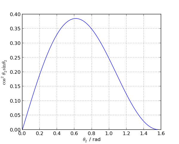
The exact form of this angular factor depends on the boundary condition applied. We have given the values for scalar-wave Dirichlet ($\psi=0$) boundary conditions; scalar-wave von Neumann and polarised waves give different forms. However, they always include a factor $\sin\theta_{2}$ for simple geometric reasons, so that long-wavelength roughness doesn’t cause much loss. Likewise, since $\sin\theta_{2}$ can’t be bigger than 1, wavenumbers bigger than $k$ don’t contribute at all.

Let us suppose that the power noise spectrum is an isotropic Gaussian, peaked at very long wavelengths:

$\displaystyle P(k_{x},k_{y})=\sigma^{2}\frac{\lambda_{C}^{2}}{\pi}e^{-\lambda_{C}^{2}(k_{x}^{2}+k_{y}^{2})}$

(17)

where $\lambda_{C}$ is a correlation length and $\sigma$ is an amplitude parameter, and the normalisation condition is $\iint P(kx,ky){\rm d}k_{x}{\rm d}k_{y}=\sigma^{2}$. Plugging this into Eqn. (15):

	$\displaystyle\Lambda=$	$\displaystyle\int_{\theta_{3}=0}^{2\pi}\int_{\theta_{2}=0}^{\pi/2}{4k^{4}\cos^{2}\theta_{2}\sin\theta_{2}}\sigma^{2}\frac{\lambda_{C}^{2}}{\pi}e^{-\lambda_{C}^{2}\sin^{2}\theta_{2}(k^{2}\cos^{2}\theta_{3}+k^{2}\sin^{2}\theta_{3})}{\rm d}\theta_{2}\,{\rm d}\theta_{3}$		(18)
	$\displaystyle=$	$\displaystyle 8k^{4}\sigma^{2}\lambda_{C}^{2}\int_{\theta_{2}=0}^{\pi/2}{\cos^{2}\theta_{2}\sin\theta_{2}}\,e^{-\lambda_{C}^{2}k^{2}\sin^{2}\theta_{2}}{\rm d}\theta_{2}$		(19)

We perform the final integral in Mathematica, giving the Dawson $F$ function ($D_{+}$), which is never bigger in magnitude than 0.5, and for large arguments $\lambda_{C}^{2}k^{2}\gg 1$ tends to small values.

$\displaystyle\Lambda=$

$\displaystyle 8k^{4}\sigma^{2}\lambda_{C}^{2}\left[\frac{1}{2\lambda_{C}^{2}k^{2}}-\frac{D_{+}(\lambda_{C}k)}{2\lambda_{C}^{3}k^{3}}\right]$

(20)

For $\lambda_{C}k\ll 1$, $D_{+}(\lambda_{C}k)\sim\lambda_{C}k$ and therefore $\Lambda\to 0$ as expected. For $\lambda_{C}k\simeq 1$ we get $D_{+}(\lambda_{C}k)\simeq 0.5$ and $\lambda_{C}^{2}k^{2}\simeq\lambda_{C}^{3}k^{3}$, therefore recovering the expected Debye-Waller factor $\Lambda\simeq 2k^{2}\sigma^{2}$. For $\lambda_{C}k\gg 1$, $D_{+}(\lambda_{C}k)\to 0.5$ and an extra factor of 2 appears giving $\Lambda\simeq 4k^{2}\sigma^{2}$. Note that in the limit $\lambda_{C}k\gg 1$, the scattering loss becomes independent of $\lambda_{C}$. The physical origin of this additional factor of 2 in the limit $\lambda_{C}k\gg 1$ compared to the usual Debye-Waller factor is not immediately clear to us, but we do not discuss this discrepancy in detail here.

Note that this derivation assumes a Gaussian power spectral density for the roughness, but does not strictly assume Gaussian-distributed heights. The surface roughness should be measured with a length scale which is comparable to, but not shorter than, the incident wavelength.

From Equations 12 and 15, calculating the expected loss is from a high-precision measurement of a mirror profile is straightforward. Equation 12 is simply the Fourier transform of the mirror surface profile for which numerically-efficient packages are available in most programming languages. Finally, we express $\theta_{2}$ and $\theta_{3}$ in terms of $k_{x}$ and $k_{y}$, noting that $kA=k_{x}$ and $kB=k_{y}$. We use the Jacobian to transform the integral over $(\theta_{2},\theta_{3})$ to an integral over $(k_{x},k_{y})$, yielding

$\displaystyle\Lambda=\iint{4k\sqrt{k^{2}-k_{x}^{2}-k_{y}^{2}}(k_{x}^{2}+k_{y}^{2})P(k_{x},k_{y})}{\rm d}k_{x}\,{\rm d}k_{y}$

(21)

where $P(k_{x},k_{y})$ is the two-dimensional Fourier transform of the surface profile. It is again clear that there is very little scattering loss from roughness with small wave-vector (this roughness simply appears as a global shaping of the mirror surface, allowing good reflection), and no scattering for large wavevectors of roughness (the incident light has too long a wavelength to probe roughnesses on short scales).

References

- [1] Peter Debye. Interferenz von röntgenstrahlen und wärmebewegung. Annalen der Physik, 348(1):49–92, 1913.
- [2] Ivar Waller. Zur frage der einwirkung der wärmebewegung auf die interferenz von röntgenstrahlen. Zeitschrift für Physik, 17(1):398–408, 1923.
- [3] Harry J Lipkin. Physics of debye-waller factors. arXiv preprint cond-mat/0405023, 2004.
- [4] JA Ogilvy. Theory of Wave Scattering from Random Rough Surfaces. Adam Hilger, 1991.