ICAS 050/20
-explorer : a simple tool to probe models
against LHC data
Ezequiel Alvarez†, Mariel Estévez⋄, Rosa María Sandá Seoane⋆,
International Center for Advanced Studies (ICAS)
UNSAM, Campus Miguelete, 25 de Mayo y Francia, (1650) Buenos Aires, Argentina
E-mail: sequi@unsam.edu.ar, mestevez@unsam.edu.ar. rsanda@unsam.edu.ar,
Abstract
New Physics model building requires a vast number of cross-checks against available experimental results. In particular, new neutral, colorless, spin-1 bosons , can be found in many models. We introduce in this work a new easy-to-use software -explorer which probes models to all available decay channels at LHC. This program scrutinizes the parameter space of the model to determine which part is still allowed, which is to be shortly explored, and which channel is the most sensitive in each region of parameter space. User does not need to implement the model nor run any Monte Carlo simulation, but instead just needs to use the mass and its couplings to Standard Model particles. We describe -explorer backend and provide instructions to use it from its frontend, while applying it to a variety of models. In particular we show -explorer application and utility in a sequential Standard Model, a B-L and a simplified two-sector or Warped/Composite model. The output of the program condenses the phenomenology of the model features, the experimental techniques and the search strategies in each channel in an enriching outcome. We find that compelling add-ons to the software would be to include correlation between decay channels, low-energy physics results, and Dark Matter searches. The software is open-source ready to use, and available for modifications, improvements and updates by the community.
1 Introduction
The Large Hadron Collider (LHC) is an outstanding and successful machine with countless achievements including the discovery of the Higgs boson [1, 2] as one of the most emblematic. In its current stage, the LHC is exploring unsurveyed energies and luminosities in its quest for discovering New Physics (NP). One of the few conclusions that could be withdrawn from current results is that many theoretical forecasts have not been fulfilled so far, and searches should address a more phenomenological and perhaps general point of view.
One expected NP signature in many NP models and also from a general phenomenological point of view is a neutral colorless spin-1 particle, also known as a [3, 4] because of its similarity in quantum numbers to the Standard Model (SM) boson. The objective of this work is to develop a tool which can be used to test against current experimental results any model predicting a particle. One of the main objectives pursued in this work is to create a very simple tool which could be learned and used rapidly to explore parameter space while constructing NP models or exploring pure phenomenology. The only input required to test a model from this phenomenological point of view would be its couplings and/or branching ratios to the allowed decaying channels.
Because of the quantum numbers, its possible decay channels explored at the LHC and their corresponding latest results are [5, 6, 7], [8], [9, 10], [11, 12], [11, 12], [13, 14], [15, 16], [16]. Since testing all these channels while constructing a model it is cumbersome, we study in this manuscript a new tool which would facilitate this enterprise.
To tackle this problem we observe that each decay channel has different sensitivity not only because of the specific detector and experimental techniques to reconstruct each particle, but also because of the different SM backgrounds affecting each final state, and because all of these depend on the mass of the sought . Although all these features for each channel are individually complex, and still more when combined, their relevant features are summarized in the exclusion plots presented by the experimental groups in each search. We show that using this information we can estimate in a reasonable way whether a point in parameter space in a NP model is excluded or not, and which of the above is the most sensitive channel. On this basis, along this work we present the software -explorer which can make the mentioned computation automatically in a very simple manner and for a huge amount of points in parameter space.
There are available software which also aim to test NP models against available experimental data in a simple manner with connection to our proposal [17, 18, 19, 20, 21, 22, 23]. Many of them are for specific NP models –such as for instance supersymmetry– and others for specific processes –such as Dark Matter portal. Refs. [21] and [23] are designed for general purpose models. Ref. [21] is a very complete software analyzing a variety of NP signatures, however the module only addresses the dilepton and dijet channels. On the other hand, recent Ref. [23] also includes interesting finite width and interference effects, however its current analysis is restricted to dilepton final states. In the present manuscript, although our mechanism is more simplified than others in some aspects, it is reasonably solid and we analyze simultaneously all possible decay channels while providing the quantitative strength for each one of them.
This article is organized as follows. In Sect. 2 we briefly review LHC searches and their sensitivity, also focusing on some other specific topics relevant for our purposes. In Sect. 3 we make a full description of our software. In Sect. 4, we apply our results to three different models: the Sequential Standard Model (SSM), a B-L model and a two-sector or Warped/Composite Model. In Sect. 5 we present the outlook of our results, and discuss future possible prospects. Finally, Sect. 6 contains the conclusions. We include in Appendix A, as a working example, a computation of the strength for the Higgs boson discovery using the previous year data and predict which channel would discover it.
2 LHC Z’ searches and sensitivity
The aim of this article is to present -explorer , a simple software that determines the most sensitive channel for the exclusion (or detection) of a boson. -explorer can analyze any point in parameter space of NP models given by the user. With the purpose of better understanding -explorer functioning as explained in next sections, we briefly describe in the following paragraphs how LHC searches are addressed and introduce related topics needed to understand the software building.
A resonance is produced at the LHC through quark-antiquark annihilation. Therefore its production cross-section depends on its coupling to valence and sea quarks, , , , and , which depend on the point in parameter space in the NP Lagrangian. Since is a spin-1 particle, it cannot be produced at loop level through gluon fusion because of Landau-Yang theorem [24, 25, 26]
decay modes and branching ratios also depend on the specific NP model. decay to dijets depends on the above mentioned coupling to quarks, but its branching ratios also depends on the coupling to all other particles The search of a at the LHC, as for any other NP particle, is implemented in different decay channels. At the LHC, searches have been performed both by the CMS and the ATLAS Collaborations, and have superseded the results coming from searches in other colliders such as Tevatron in most of the TeV scale [27].
Although the fraction of times a decays to a given channel depends solely on its corresponding branching ratio, in experimental terms the acceptance and efficiency of the detector and the background of this channel are crucial to determine its exclusion/discovery sensitivity. These features also have an important dependence on the scale of energies considered, which depends on the sought resonance mass. For instance, for the search of a with TeV at the LHC, we expect the dijet channel to have large QCD background, which dominates at low . Whereas in the dilepton channel, the background is smaller in comparison, and thus the signal is likely cleaner and the channel more sensitive even though its branching ratio could be smaller. Considering also the decay mode, for the same above reasons the fully hadronic decay is hidden in QCD background, whereas the leptonic decays, although cleaner, are difficult to reconstruct due to missing energy. This scenario changes for larger masses, TeV. In such a case there is a more subtle interplay between the features discussed above. Not only because all backgrounds are highly reduced, but also because the techniques for detecting and reconstructing particles are also modified. In particular, in this high regime, boosted massive particles, such as boson or quark, can decay hadronically in configurations where all particles are collimated in a single fat jet, which is more distinguishable from QCD background. This, in conjunction to a reduced QCD background yields a favorable enhancement for channels such as hadronic and top.
From this overview on some of the features involved in determining which is the best channel to exclude (or find) a given , we see that there are a variety of non-trivial ingredients which affect which channel could be the most sensitive. It is of particular interest for our work to determine a magnitude that condenses all the relevant information and provides an estimation on the sensitivity of each channel for each point in parameter space in a given NP model. From the phenomenological point of view, the information available on previous experimental searches in the different channels at a given energy and luminosity can be incorporated into the determination of the most sensitive decay channel, through the extraction of the predicted experimental limits. With this, the strength () of the signal of each channel can be defined as [28]
| (1) |
where is the predicted cross-section times branching ratio times acceptance of the new , and is the corresponding predicted experimental upper limit at the CL. Despite the complex compromise between the expected theoretical branching ratio and the cleanliness of the experimental signal coded in its definition, the strength S has a simple interpretation. If for a given channel for a given point in the parameter space, the point is experimentally excluded. But if for all channels, the point is not only not excluded but also the one with the largest is expected to be the most sensitive channel for the exclusion or observation of the particle being sought. We illustrate this statement in Appendix A by using the data from the year previous to the Higgs discovery.
The difference in using predicted instead of measured limits consists in considering the experimental techniques instead of eventual fluctuations in the data. In case the measured limit departs significantly from the predicted value, it would correspond to a discovery or a wrong prediction which in both cases should be addresses from another point of view.
Ideally, for this comparative analysis between all possible final states for a particle, it is expected that for a given energy the experimental measurements for each channel will be at the same luminosity, but this is not always the case. However, these luminosities tend to be almost within the same order of magnitude, so assuming a statistical uncertainty regime, the experimental sensitivity can be rescaled with the square root of the ratio of the luminosities [28].
| (2) |
See also Appendix A where this assumption is verified in a real case scenario.
3 -explorer software
Motivated by the discussion and strength () definition in previous section, we have designed a simple software that, for a given NP model, it can compare the sensitivity of available channels. Along this section we describe how this software works and how it can be utilized by any user to extract useful and relevant information for any model.
3.1 Backend
-explorer is a C++ open source program [29] that allows to determine the most sensitive channel for the search of a boson at LHC as a function of the relevant NP parameters in the model: the mass of the boson (), the couplings of to all SM-fermions and the decay widths to diboson and neutrinos and/or invisible.
-explorer running flow is quite simple. Using the above input parameters, the program computes the production cross section for and the different decay rates to each one of the considered channels, which are: , , , , , , (or any invisible), and . Once this is obtained, these predictions for each possible final state are compared to the corresponding upper limit on the product of the cross section times branching fraction, coming from the most sensitive searches performed both by the ATLAS and CMS collaborations. The comparison is made through the calculus of the aforementioned strength , explained in Sect. 2.
To compute the production cross section, the program uses previously generated and recorded production cross section with MadGraph5_aMC@NLO [30] with a tailored model which couples with unity to only one quark in the proton each time and for a set of values of between 0.4 and 8.1 TeV, with a step of 0.01 TeV, and at TeV. Since LHC protons are unpolarized we set same couplings for Left and Right chiralities at this level. These calculus, stored in the repository as /cards/sim_cards, are used during program execution: the predicted production cross section for a specific reference point is the sum of the five contributions of quarks (, , , and ). Each of them adjusted by the sum of the corresponding squared chiral couplings, that are extracted from the input card. The software selects inside the simulations the record with the mass that is closest to the one in the input card at the corresponding reference point. The total production cross section is then used in each possible decay channel to compute the needed in Eq. 1, multiplying by the corresponding branching ratio, which is calculated by the program using the input parameters.
The experimental limits used by the program, corresponding to the value of required in Eq. 1, are stored in /cards/exp_cards. The searches included in the program, performed by both ATLAS and CMS collaborations and considering the latest results up to date, include the following channels and references: [5], [8], [9], [11], [11], [13], [15], [16]. We use the digitalization [31] of the numerical values of upper limits on the product of the cross section and the branching fraction versus from the corresponding published plots. It is worth noticing that since searches are constantly updated, the user can modify the experimental limits for a given channel just by modifying the corresponding exp_card and propose the update of the repository. The program includes a README file in which the numeric labeling of exp_card for each channel is displayed.
3.2 Frontend
One of the main features of our software is its simplicity. The user only has to provide an input card as /incard/card_1.dat, specifying (in TeV), the couplings to all SM-fermions (except for neutrinos, which information is required through ), and the partial widths to () and (). We require this latter information as partial width since there is not a unique Lorentz structure in their couplings. The total width to non SM particles can be added in the computation as . The data should be specified as one row for each point in parameter space with the following order in each row:
where () is the coupling of to the corresponding Left (Right) fermion. There is no limit in the number of rows in the input card, and the program runs very fast and using negligible CPU resources. Each row, with its corresponding twenty-three columns, is a different reference point in the parameter space for the program.
To execute the program, once in the main directory in a Linux terminal, the user has to write in command line the following instruction:
A brief summary of the tasks performed by -explorer will be displayed on screen. The generated output file (saved in /output/1.dat), contains the same information than the input card in each line, to facilitate the subsequent processing and analysis of the generated information, followed by the calculated strength () in each channel, presented in the following order from column twenty-four to column thirty-three:
Observe that the is left as a dummy variable to eventually add new possible channels in the future.
Since each row in the input file is a different point in the parameter space for -explorer, output card contains the same number of rows of data than card_1.dat. The running time depends on this number of rows and the CPU speed, but typically for an input card of reference points, time is less than seconds.
Additionally, after running, in the /extra folder and in different files are available the estimated decay widths, branching ratios, the estimated and the extracted for each reference point in the input card. More details on these auxiliary files can be found in the README file.
4 -explorer application examples
Along this section we implement the software on a few well known models to show its potential and utility. We do not aim to explore in detail NP models and place constraints, but instead to show the software scope through some concrete simplified examples. As a matter of fact, we explore some regions in parameter space that are already discarded by other sectors, however we find it suitable for the sake of showing the richness -explorer would provide in that case. We utilize -explorer on a Sequential SM, on a B-L model and on a Warped/composite scenario.
4.1 Sequential Standard Model
As a first example to test the power of -explorer software, we present an analysis for the Sequential Standard Model (SSM) [32], where the couplings of the boson to all SM fermions are equal to those of the boson. The SSM is a reference model in experimental searches for its simplicity, and we use it as validation for our program.
In Fig. 1 we present the strength to all the fermion decay channels included in -explorer in terms of . The comparison of the sensitivities between the different experimental analyses is straightforward. Since couplings are not suppressed for light fermions, as it can be expected the dimuon and dielectron channels are the most sensitive. In particular, these results match those obtained by CMS in Ref. [11]. Comparing these two lepton channels, since experimental efficiency is slightly better for muon than electrons, there is more sensitivity in the dimuon decay channel as expected. It is interesting to notice how the channel passes in strength the channel for masses greater than TeV. The reason behind this are the well known developed experimental techniques for boosted top tagging [33]. Another interesting feature to be observed is how the dijet channel strength falls down slower than dilepton channels for larger masses, even surpassing the di-electron channel above 5 TeV. This could be associated to the backgrounds: the dijet background is mostly related to the gluon PDF in the proton, whereas the dilepton background is to the quark content in the proton PDF, and is well known that valence quarks are more likely than gluons at large . This kind of features show some aspects of all the information condensed in the strength .
Additionally, we also carried out -explorer validation using the latest ATLAS results [12], where the information for both leptonic channels is in the combined dilepton channel.
4.2 B-L model
We present the sensitivity analysis for the search at LHC of a coming from a minimal extension of the SM, associated to the B-L number. The gauge sector Lagrangian for this NP scenario is [34, 35, 36]
| (3) |
where , and are the field strength tensors for , and (ignoring the gauge symmetry for the purposes of our analysis).
In this type of models, mixing occurs through the conventional spontaneous symmetry breaking (SSB) mechanism, because the usual Higgs doublet is not singlet under the new [37]. The scalar sector is defined as
| (4) |
| (5) |
where is the aforementioned scalar doublet, and is a complex singlet scalar field required to achieved the breaking of the new gauge group to acquire a vev at the TeV scale. The covariant derivatives are [38, 34]
| (6) |
with and . After SSB, the scalar fields can be written as
where the two vev’s, and , are real and positive. From the minimization of Eq. 5 one obtains the mass matrix for and , and after its diagonalization the mass eigenstates and are obtained
Here is the mixing angle and is the SM-like Higgs boson. Along this work, we consider and thus and .
The interactions vertices between the neutral gauge bosons , and a pair of SM fermions are given by [34]
| (15) |
where the new couplings are
| (16) | ||||
and is the - mixing angle. In the limit where and , the couplings of the boson to all SM fermions are recovered. This angle is bounded by LEP searches, and the current bound on this parameter is [27]. Electro-Weak Precision Tests from LEP-II also place limits in the model and therefore we restrict our exploration to the 99% C.L. allowed region TeV [39]
The additional formulae required by -explorer are the decay widths of the new boson to [4, 40] and to [41, 40]
| (17) | ||||
| (18) | ||||
with
| (19) |
Using the above information we use -explorer to compute the strength for all channels as a function of and . In Fig. 2 we present the most sensitive channel for each region of the parameter space. There is an area excluded mainly by dimuon searches for 2 TeV 5 TeV and 0.2 0.7. It is interesting to observe that the dielectron channel only excludes points with TeV. This is intimately related to the results in Ref. [11], which is likely to be related to experimental details in the geometry and the detector’s efficiencies. In any case, the strength for dielectron and dimuon channels is very close in that region. For small and masses TeV there is a still not excluded region where dimuon is the most sensitive channel. For large masses, where there are no experimental limits for leptonic final states, the dijet channel becomes the most sensitive channel.
4.3 Warped/Composite Model
As a third example we study the phenomenology of a coming from a warped/composite or two-sector model, through -explorer. The goal in analyzing this model is to explore a NP scenario in which the couplings are related to the mass spectrum11 1 A use of -explorer in a full Composite scenarios can be found in Ref. [42], which has been completed while this project was under development.. We summarize a simplified version of a partial compositeness four dimensional model following Ref. [43] lines of reasoning and notation, where more details can be found.
This model includes, beside the ones in the SM, new fermions and bosons with masses around the TeV scale. The composite sector contains vector excitations which respect a symmetry, fermions and –one for each elementary fermion–, and the Higgs field . We use the same fermion embedding as in Ref. [43]. Our assumption is that the composite sector corresponds to a strongly interacting theory, but still perturbative. This is translated into assuming relevant NP couplings and Yukawas . Since we are interested in new neutral bosons and their couplings to the SM fermions, we should get the mass states for all the particles. To this end, we diagonalize analytically the Lagrangian before EWSB, and then diagonalize it again after including the EWSB effects. Since the neutral boson mixing matrix is we choose to perform a decomposition in terms of powers of . This should be taken cautiously to maintain consistency for given scale and parameters. The new diagonalized fermions are the SM quarks and leptons and their corresponding physical composite partners, which we do not consider here. The new diagonalized bosons correspond to the photon , the , , and the new heavy resonances which are the neutral , and (combination of , and ) and the new charged . The boson fields from the old basis can be expressed as a function of the mass eigenstates as in Eq. 24 in Appendix B.
All new ’s could be in principle easily tested through -explorer once the corresponding couplings are explicitly written. We work out as an example the phenomenology of the boson. Observe that equals at zeroth order in the vev. We therefore compute the required couplings to the SM fermions by substituting the change of basis in the Lagrangian and extracting the couplings at second order in . Couplings of the to SM fermions can be found in Eqs. 26 - 28 and its decay widths to bosons in Eq. 30, in Appendix B.
Once the Lagrangian is written in the mass eigenstate basis, the phenomenology depends in principle on the couplings and Yukawas (), the Higgs potential parameters (), the new sector mass parameters () and the mixing angles (). In the following we assume a composite fermion scale TeV, and we vary other parameters to reproduce physical parameters compatible with experimental observations. The SM couplings should satisfy
| (20) | |||||
| (21) |
The SM fermion masses, which are function of the mixing angles, , and , should reproduce the physical values. For the given setup and interest, we scan on the parameters to fit first and third generation and define the allowed regions in parameter space. A further tuning should be performed if one would like the model to also reproduce second generation and flavor physics constraints22 2 For NP masses in the order of a few TeV, this could be achieved for instance in the lines of Ref. [44].. However, for the purposes of this work, where we aim to show the utility of -explorer and not to explore the full details of the model, the outcome of this diagonalization and mixing angles is enough to capture the essence of a with varying couplings to the different generations due to mass mixing terms.
For light quarks, the scan on parameter space yields similar results for up and down quarks, selecting the region of tiny mixing angles. This is no surprising since the Yukawas and composite couplings were chosen to give strong coupling of the composite sector to the top and weak to the light fermions. For simplicity, and within the scope of our framework we can approximate for all light fermions without major modifications. Therefore, the boson would couple to these light particles through its mixing with the SM bosons. For bottom and top the situation is different. The region allowed for the bottom is similar to that of the light fermions for , but it is a different case for which should be large since otherwise the top mass cannot be large. The top quark needs both to be large in order to reproduce its mass. Therefore we find that , and , which represents a large left third generation and right top coupling to the composite sector and small right bottom coupling. This yields , and much more coupled to the composite fermions while the light SM fermions and are decoupled at this level of approximation. In light of these approximations, we scan on . Once is chosen, we determine a that reproduces the top mass within 20% of its value. Observe that within our approximation couplings do not depend on .
Finally, we can set limits to ’s angles. Since we assume , using and and the relation we obtain
| (22) | |||||
| (23) |
In the following we extend range beyond the above to explore its effects on the phenomenology through -explorer.
So far we have collected the required elements for the running of -explorer to calculate the strengths to , , , , , , , and . We fix the parameters TeV, TeV, and run from TeV, from and from (see Appendix B) to have a broad view in parameter space. Since we are working with , whose couplings have no contributions from the hypercharge sector given our approximations, parameter does not play any role (see Eqs. 26 - 28).
Ref. [43] uses couplings of fermions and bosons before the last diagonalization, as a simplified approximation. We compare the branching ratios given in that work with the ones obtained above performing the full diagonalization. We found that the widths depends on the same variables than the ones computed in Ref. [43]. Being the quark massless within our approximation, we need to go to the next order in to see a dependence on and . It can be seen that decays to light fermions and decays to bosons are opposite in behavior. For small , the decay to light fermions is small and increases with , while decay to bosons goes exactly the opposite way. The heavy quarks width is small while is small and increases for small when is larger, assimilating to the width of the bosons. This is because if is small the mixing between heavy quarks and composite heavy quarks is negligible as in the light quarks case. Whereas for larger coupling it mimics the boson behavior, which are strongly coupled to . In Fig. 3 we can see the branching fractions for our calculation. As a validity check, we verify that we recover the branching fractions in Ref. [43] in the corresponding limit.
Once the above calculations, details and validity checks for the Warped/Composite model have been performed, we can easily process the model through -explorer and analyze the strength in each channel. We show the results for -explorer output in Fig. 4. Observe that the allowed values for the physical mass obeys Eq. 25 in Appendix B. As it can be seen, four channels are the most sensitive depending on the region in parameter space. For , it is the channel, which agrees with the plot of the branching ratios in Fig. 3, since this final state has a considerable larger fraction than other channels for small . The region for large mass and small in which is the most sensitive channel is because there is no data for at these masses in the -explorer experimental cards. In addition, for small the channel is preferred over , due to the BR dependence on as can be seen in Fig. 3. The undefined region for small and is because of variations in the non-plotted angle which modifies the branching ratios. This is for the range indicated in Eq. 23, however, for the sake of the phenomenological interest, we also analyze the whole plot for . As increases above there is an interplay between the branching ratio increase in Fig. 3 and its sensitivity, becoming this final state the most sensitive channel (largest strength). In some part of the parameter space –smaller masses, black color in Fig. 4– the model is discarded by , whereas in the other part is still allowed and also is the most sensitive channel. As goes above 5.5 TeV, there are no results and channel becomes the most sensitive one. The dijet final state also has a considerable increase in its branching ratio in this region.
As it can be seen in this last result (Fig. 4) for a simplified warped/composite model, the software -explorer condenses a large amount of information regarding the model itself and the experimental techniques for each specific channel, into one number –the strength– which yields a plot with the relevant information for the phenomenological analysis of the model.
5 Outlook
Along the previous paragraphs we have presented a software for performing simplified testings of BSM models in light of recent LHC experimental results. We discuss in this section limitations and potential improvements of this software.
A direct limitation of -explorer is that in the aim of being general, its predictions are at leading order tree level. This limitation cannot be avoided in a program which is for general BSM models, since any NLO effect is model dependent. In fact, NLO effects through loop-level corrections depends on the full particle content in the model. However, it should be noted that if users need to include NLO effects while running -explorer, they can do it by computing the NLO branching ratios and adapting the -explorer input cards. The couplings corresponding to each point in parameter space should be re-scaled accordingly, and analogously the widths.
On the other hand, there are interesting add-ons which would enhance -explorer utility. One possibility is to schematically include low energy observables as bounds on the models. Although this is a vast enterprise, it would be very appealing to have all these limits collected in an easy-to-run software such as -explorer. Another compelling possibility is to include Dark Matter searches with as mediator, or as DM candidate [45].
An important add-on for -explorer would be to include cross-correlations in the analysis. Since it could be the case that, because of small cross-sections, a NP model is recognized by slight excesses in different specific channels. This undertaking would also require to cross-correlate the backgrounds since in many cases different channels have the same background. We consider that this is a very attractive add-on for a finder software, and it would have to be done to fully explore the available experimental data in contrast to NP models.
Our code is open-source [29] and any of these updates can be done by interested users. We are willing to contribute or assist.
6 Conclusions
We have designed a new software -explorer to easily test NP models with a boson against experimental constraints in all decay channels that can be measured at LHC. The main idea of this tool is to extract the bounds in production times branching ratio times acceptance from the ATLAS and CMS results and apply them systematically to the NP model. The basic input for -explorer is a point in parameter space with the relevant phenomenological information, and the program returns as output a positive number for each channel, which is its corresponding strength. If this number is larger than 1, means that the point in parameter space is rejected by the corresponding channel. Moreover, the sensitivity to the given point in parameter space in each channel may be compared by studying the strength in each channel: the larger the strength, the more sensitive is the channel to reject (or observe) the NP model.
The program does not need the user to input the model, nor run any Monte Carlo simulation. Instead, just needs the mass, couplings to charged fermions and partial widths to invisible, and , in a simple text file, where each row is a different point in parameter space to be tested. -explorer is intended to be as simple as possible, and therefore very fast: in a normal computer it can process 1000 points in a few seconds. The whole program is open source written in c++ and can be used, modified and improved by other users through its Github interface [29].
We have validated -explorer by applying it to the Sequential Standard Model (SSM) and re-obtained available results shown in Fig. 1. We have also worked out two other examples to explicitly show the functioning and scope of the program. We have applied -explorer to a B-L model (Fig. 2), and to a 2-sector or Warped/Composite model. In both cases we have sketched the required work before running the software, which consists in identifying the mass eigenstate , its couplings to SM fermions, and its width to SM bosons. The running of -explorer on these NP models and the corresponding analysis of its output, has shown how -explorer condenses the theoretical side of the model, and the experimental techniques for each channel including its relevant backgrounds, exhibiting the power of the presented tool. Many of these features are accordingly discussed along the text.
We have discussed benefits and issues of such a straightforward software and how in some cases the problems may have a workaround. We have also discussed different possible improvements to -explorer. We consider that including correlation between channels, low-energy physics results and Dark Matter bounds, would be very compelling.
The main objective of the presented software -explorer is to provide a useful tool for theorist and experimentalist to test NP models against LHC data.
Acknowledgments
We thank Leandro Da Rold and J. Lorenzo Díaz-Cruz for useful conversations. E.A. thanks Manuel Szewc for testing the software, M.E. thanks Nicolás Echebarrena for assistance with the code, and R.M.S.S. thanks Diego Mouriño for helping with Github.
Appendix A Strength example in Higgs Boson discovery
As a concrete example on the utility of the strength defined in Eq. 1, we use it to study relevant features in the prediction of the 2012 Higgs boson discovery using experimental data available in 2011.
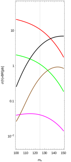
We show in Fig. 5a the predicted branching ratios of the Higgs boson as a function of its (then unknown) mass. Although is the main decay channel for a 125 GeV Higgs boson, its background is very large at the LHC, and therefore it is an unlikely channel for its discovery. On the other hand and have a non negligible branching ratio and background not too large, albeit that the channel does not have the power to predict the resonance mass due to the missing energy leaving the detector as neutrinos. The particular case is channel which has a tiny branching ratio, but also a tiny background, therefore being a very likely channel for discovery. This qualitative discussion can be taken to a quantitative analysis by simply using the strength .
(a)
(b)
In order to perform a quantitative analysis using , we extract a zoom of the Higgs decay channels for the relevant region in masses and channels in Fig. 5b left panel. To these results we apply the computation of the strength. We multiply by the acceptance and divide by the 2011 LHC predicted 95% C.L. limits in cross-sections branching ratio acceptance in each channel. We obtain these latter limits by either the numeric available data or by digitalizing the 2011 available experimental results in [46] (7 TeV, 1.1 fb-1) , (7 TeV, 4.7 fb-1) [47], [48] (7 TeV, 4.6 fb-1), [49] (7 TeV, 4.6 fb-1) and [50] (7 TeV, 1.09 fb-1), where all data has been normalized to luminosity 4.7 fb-1 using Eq. 2. The outcome of the strength is plotted in Fig. 5b right panel. In this figure it can be seen which is the 2011 discovery prediction using strength: the first channel where a 125 GeV is going to be observed is , and then shortly after in and simultaneously.
The Higgs boson was discovered in 2012 using 4.8 fb-1 (7 TeV) and 5.8 fb-1 (8 TeV) of luminosity by ATLAS [1] and 5.1 fb-1 (7 TeV) and 5.3 fb-1 (8 TeV) by CMS [2]. Although the more impressive channels were and because a resonant peak could be distinguished at 125 GeV, the excess in was available before, as predicted by the strength analysis in previous paragraph and in Fig 5b. This can be seen in Fig. 6, where we have put aside for comparison the observed and expected limits for and at same luminosity and energy conditions. The channel is already measuring the Higgs excess, although it does not show any resonant peak because of the missing energy in the decay products.

Along this concrete example of the Higgs boson discovery we have shown the usage and utility of the strength. We present the agreement between the 2011 predictions and the 2012 experimental results, as an estimate example on how could work a simple analysis using strength in predicting features of an eventually yet unobserved new resonance using -explorer .
Appendix B couplings and widths to SM particles
In this Appendix we expand some of the details of the neutral gauge boson in the Warped/Composite framework.
We perform the expansion of the fermions eigenvectors to second order in . In the case of the bosons, the first order is zero because in the original matrix the vev already appears quadratic, and hence we also keep here to second order. The boson fields from the previous basis, written as a function of the new mass eigenstates read, up to a normalization constant,
| (24) | ||||
where the parameters are the same as those used in Ref. [43]. The physical masses of the and the photon are the usual while for the new they are given by
| (25) |
We can obtain the couplings to bosons and fermions by substituting the old bosons for the mass states after the diagonalization. We extract the couplings at second order in and work in the region to assure the validity of the perturbative expansion. Since in our scanning 1 TeV is the lowest bound for the parameter, we take .
Since we consider all fermions but the top as massless, we use except . Analogously, we take . This simplifies the model and yields a better understanding of the couplings behavior. We can see that all light fermions have a similar coupling, with the Left ones having an extra term coming from their interaction. The top quark has extra terms in both chiralities because of the non vanishing Yukawa, and the Left chirality because of . The same goes for the bottom, except that since this is a massless quark, its Yukawa being zero makes zero extra terms and also .
Couplings to light quarks, are given by
| (26) | ||||
Within our level of approximation we consider the above couplings for first and second generations.
The couplings to the third generation of quarks are given in Eq. 27, where the top is considered heavy and the bottom massless.
| (27) | ||||
Here is the diagonalized mass.
Finally, couplings to all leptons are given in Eq. 28, where the three generations are considered light.
| (28) | ||||
In order to use the -explorer software in this framework, we need to find the decay width of the to SM bosons. The easiest way is considering the Equivalence Theorem [53], which states that the longitudinal and are equivalent to the corresponding Goldstone Bosons in the high energy limit. As a consequence, the widths are given by
| (29) |
Notice that these widths corresponds to the decay, and not the new mass states. To get the width corresponding to the physical states, one needs to perform the diagonalization and extract the couplings of the new to the SM bosons. This is not straightforward, since one should also consider the gauge Lagrangian and the rotations of the charged bosons. For the sake of simplicity, we use the approximation for high masses in which is mainly composed of (see Eq. 24), while the contribution from and quickly decays to zero. A larger assures that is small and therefore a fast convergence. For the case of smaller masses, we found that for small angles the three neutral boson masses are of the same order. We therefore choose to analyze phenomenology and approximate the following decay widths as
| (30) |
References
- [1] ATLAS collaboration, G. Aad et al., Observation of a new particle in the search for the Standard Model Higgs boson with the ATLAS detector at the LHC, Phys. Lett. B716 (2012) 1–29, [1207.7214].
- [2] CMS collaboration, S. Chatrchyan et al., Observation of a New Boson at a Mass of 125 GeV with the CMS Experiment at the LHC, Phys. Lett. B716 (2012) 30–61, [1207.7235].
- [3] P. Langacker, The Physics of Heavy Gauge Bosons, Rev. Mod. Phys. 81 (2009) 1199–1228, [0801.1345].
- [4] A. Leike, The Phenomenology of extra neutral gauge bosons, Phys. Rept. 317 (1999) 143–250, [hep-ph/9805494].
- [5] ATLAS collaboration, G. Aad et al., Search for new resonances in mass distributions of jet pairs using 139 fb-1 of collisions at TeV with the ATLAS detector, 1910.08447.
- [6] CMS collaboration, C. Collaboration, A search for dijet resonances in proton-proton collisions at with a new background prediction method, .
- [7] ATLAS collaboration, M. Aaboud et al., Search for low-mass dijet resonances using trigger-level jets with the ATLAS detector in collisions at TeV, Phys. Rev. Lett. 121 (2018) 081801, [1804.03496].
- [8] ATLAS collaboration, M. Aaboud et al., Search for resonances in the mass distribution of jet pairs with one or two jets identified as -jets in proton-proton collisions at TeV with the ATLAS detector, Phys. Rev. D98 (2018) 032016, [1805.09299].
- [9] CMS collaboration, A. M. Sirunyan et al., Search for resonant production in proton-proton collisions at TeV, JHEP 04 (2019) 031, [1810.05905].
- [10] ATLAS collaboration, M. Aaboud et al., Search for heavy particles decaying into top-quark pairs using lepton-plus-jets events in proton–proton collisions at TeV with the ATLAS detector, Eur. Phys. J. C78 (2018) 565, [1804.10823].
- [11] CMS Collaboration collaboration, Search for a narrow resonance in high-mass dilepton final states in proton-proton collisions using 140 of data at , Tech. Rep. CMS-PAS-EXO-19-019, CERN, Geneva, 2019.
- [12] ATLAS collaboration, G. Aad et al., Search for high-mass dilepton resonances using 139 fb-1 of collision data collected at 13 TeV with the ATLAS detector, Phys. Lett. B796 (2019) 68–87, [1903.06248].
- [13] ATLAS collaboration, M. Aaboud et al., Search for additional heavy neutral Higgs and gauge bosons in the ditau final state produced in 36 fb-1 of pp collisions at TeV with the ATLAS detector, JHEP 01 (2018) 055, [1709.07242].
- [14] CMS collaboration, V. Khachatryan et al., Search for heavy resonances decaying to tau lepton pairs in proton-proton collisions at TeV, JHEP 02 (2017) 048, [1611.06594].
- [15] ATLAS collaboration, M. Aaboud et al., Search for resonance production in final states in collisions at 13 TeV with the ATLAS detector, JHEP 03 (2018) 042, [1710.07235].
- [16] CMS collaboration, A. M. Sirunyan et al., Combination of CMS searches for heavy resonances decaying to pairs of bosons or leptons, Phys. Lett. B798 (2019) 134952, [1906.00057].
- [17] S. Kraml, S. Kulkarni, U. Laa, A. Lessa, W. Magerl, D. Proschofsky-Spindler et al., SModelS: a tool for interpreting simplified-model results from the LHC and its application to supersymmetry, Eur. Phys. J. C74 (2014) 2868, [1312.4175].
- [18] M. Papucci, K. Sakurai, A. Weiler and L. Zeune, Fastlim: a fast LHC limit calculator, Eur. Phys. J. C74 (2014) 3163, [1402.0492].
- [19] M. Drees, H. Dreiner, D. Schmeier, J. Tattersall and J. S. Kim, CheckMATE: Confronting your Favourite New Physics Model with LHC Data, Comput. Phys. Commun. 187 (2015) 227–265, [1312.2591].
- [20] D. Dercks, N. Desai, J. S. Kim, K. Rolbiecki, J. Tattersall and T. Weber, CheckMATE 2: From the model to the limit, Comput. Phys. Commun. 221 (2017) 383–418, [1611.09856].
- [21] D. Barducci, G. Belanger, J. Bernon, F. Boudjema, J. Da Silva, S. Kraml et al., Collider limits on new physics within micrOMEGAs_4.3, Comput. Phys. Commun. 222 (2018) 327–338, [1606.03834].
- [22] J. M. Butterworth, D. Grellscheid, M. Krämer, B. Sarrazin and D. Yallup, Constraining new physics with collider measurements of Standard Model signatures, JHEP 03 (2017) 078, [1606.05296].
- [23] F. Kahlhoefer, A. Mück, S. Schulte and P. Tunney, Interference effects in dilepton resonance searches for Z′ bosons and dark matter mediators, JHEP 03 (2020) 104, [1912.06374].
- [24] L. D. Landau, On the angular momentum of a system of two photons, Dokl. Akad. Nauk Ser. Fiz. 60 (1948) 207.
- [25] C.-N. Yang, Selection Rules for the Dematerialization of a Particle Into Two Photons, Phys. Rev. 77 (1950) 242.
- [26] P. J. Fox, I. Low and Y. Zhang, Top-philic forces at the LHC, JHEP 03 (2018) 074, [1801.03505].
- [27] Particle Data Group collaboration, M. Tanabashi et al., Review of Particle Physics, Phys. Rev. D98 (2018) 030001.
- [28] E. Alvarez, L. Da Rold, J. Mazzitelli and A. Szynkman, Graviton resonance phenomenology and a pseudo-Nambu-Goldstone boson Higgs at the LHC, Phys. Rev. D95 (2017) 115012, [1610.08451].
- [29] E. Alvarez, M. Estevez and R.M. Sanda Seoane, source scripts for software in this work, GIT repository https://github.com/ro-sanda/Z--explorer.
- [30] J. Alwall, R. Frederix, S. Frixione, V. Hirschi, F. Maltoni, O. Mattelaer et al., The automated computation of tree-level and next-to-leading order differential cross sections, and their matching to parton shower simulations, JHEP 07 (2014) 079, [arXiv:1405.0301].
- [31] P. Uwer, EasyNData: A Simple tool to extract numerical values from published plots, 0710.2896.
- [32] G. Altarelli, B. Mele and M. Ruiz-Altaba, Searching for New Heavy Vector Bosons in Colliders, Z. Phys. C45 (1989) 109. [Erratum: Z. Phys.C47,676(1990)].
- [33] ATLAS collaboration, M. Aaboud et al., Performance of top-quark and -boson tagging with ATLAS in Run 2 of the LHC, Eur. Phys. J. C 79 (2019) 375, [1808.07858].
- [34] A. Gutiérrez-Rodríguez and M. A. Hernández-Ruiz, resonance and associated production at future Higgs boson factory: ILC and CLIC, Adv. High Energy Phys. 2015 (2015) 593898, [1506.07575].
- [35] L. Basso, Phenomenology of the minimal B-L extension of the Standard Model at the LHC. PhD thesis, Southampton U., 2011. 1106.4462.
- [36] S. Khalil, Low scale - L extension of the Standard Model at the LHC, J. Phys. G35 (2008) 055001, [hep-ph/0611205].
- [37] T. G. Rizzo, phenomenology and the LHC, in Proceedings of Theoretical Advanced Study Institute in Elementary Particle Physics : Exploring New Frontiers Using Colliders and Neutrinos (TASI 2006): Boulder, Colorado, June 4-30, 2006, pp. 537–575, 2006. hep-ph/0610104.
- [38] L. Basso, S. Moretti and G. M. Pruna, A Renormalisation Group Equation Study of the Scalar Sector of the Minimal B-L Extension of the Standard Model, Phys. Rev. D82 (2010) 055018, [1004.3039].
- [39] G. Cacciapaglia, C. Csaki, G. Marandella and A. Strumia, The Minimal Set of Electroweak Precision Parameters, Phys. Rev. D 74 (2006) 033011, [hep-ph/0604111].
- [40] V. Barger and K. Whisnant, Heavy-z-boson decays to two bosons in superstring models, Phys. Rev. D 36 (Dec, 1987) 3429–3437.
- [41] V. Barger, P. Langacker and H.-S. Lee, Six-lepton Z-prime resonance at the LHC, Phys. Rev. Lett. 103 (2009) 251802, [0909.2641].
- [42] L. Da Rold and F. Lamagna, A vector leptoquark for the B-physics anomalies from a composite GUT, JHEP 12 (2019) 112, [1906.11666].
- [43] R. Contino, T. Kramer, M. Son and R. Sundrum, Warped/composite phenomenology simplified, JHEP 05 (2007) 074, [hep-ph/0612180].
- [44] R. Barbieri, D. Buttazzo, F. Sala, D. M. Straub and A. Tesi, A 125 GeV composite Higgs boson versus flavour and electroweak precision tests, JHEP 05 (2013) 069, [1211.5085].
- [45] We thank V. Martin Lozano for this suggestion that will correspond to a future update.
- [46] CMS collaboration, Search for Higgs Boson in VH Production with H to bb, .
- [47] CMS collaboration, C. Collaboration, Search for a Higgs boson produced in the decay channel 4l, .
- [48] CMS collaboration, C. Collaboration, Search for the Higgs Boson in the Fully Leptonic Final State, .
- [49] CMS collaboration, C. Collaboration, Search for Neutral Higgs Bosons Decaying to Tau Pairs in pp Collisions at sqrts=7 TeV, .
- [50] CMS collaboration, Search for a Higgs boson decaying into two photons in the CMS detector, .
- [51] ATLAS collaboration, G. Aad et al., Search for the Standard Model Higgs boson in the two photon decay channel with the ATLAS detector at the LHC, Phys. Lett. B705 (2011) 452–470, [1108.5895].
- [52] ATLAS collaboration, Search for the Higgs boson in the HWWlnln decay mode with the ATLAS Detector, .
- [53] K. Riesselmann, Higgs physics and the equivalence theorem, in Perspectives for electroweak interactions in e+ e- collisions. Proceedings, Ringberg Workshop, Tegernsee, Germany, February 5-8, 1995, pp. 0175–190, 1995. hep-ph/9504321.