Dynamical Systems Theory and Algorithms for NP-hard Problems
Abstract
This article surveys the burgeoning area at the intersection of dynamical systems theory and algorithms for NP-hard problems. Traditionally, computational complexity and the analysis of non-deterministic polynomial-time (NP)-hard problems have fallen under the purview of computer science and discrete optimization. However, over the past few years, dynamical systems theory has increasingly been used to construct new algorithms and shed light on the hardness of problem instances. We survey a range of examples that illustrate the use of dynamical systems theory in the context of computational complexity analysis and novel algorithm construction. In particular, we summarize a) a novel approach for clustering graphs using the wave equation partial differential equation, b) invariant manifold computations for the traveling salesman problem, c) novel approaches for building quantum networks of Duffing oscillators to solve the MAX-CUT problem, d) applications of the Koopman operator for analyzing optimization algorithms, and e) the use of dynamical systems theory to analyze computational complexity.
Keywords: Computational Complexity, Dynamical Systems Theory, NP-hardness, Heuristic Algorithms, Combinatorial Optimization.
1 Introduction
Dynamical systems theory and computational complexity have, predominantly, been developed as independent areas of research over the last century with little interaction and mutual influence. Dynamical systems theory has its origins in the seminal work of Henri Poincaré Cit:Poincare on celestial mechanics. Computational complexity theory, on the other hand, originated in the works of Alan Turing Cit:Turing and Alonzo Church Cit:Church in the 1930s and has played an intimate role in the computing revolution of the twentieth century.
Eventually, dynamical systems theory (or nonlinear dynamics) found broad application beyond celestial mechanics. In particular, it has been used extensively to model and analyze engineering systems Cit:Stro, physics of natural phenomena, biological Cit:Bio and chemical processes Cit:chem, fluid dynamics Cit:turb, and epidemiology Cit:epi to name a few. Moreover, the analysis of dynamical systems is typically intimately tied to numerical methods Cit:set_oriented; Cit:Igor and scientific computation Cit:scientific_comp.
Links to the applications (outlined in the previous paragraph) have played a critical role in the theoretical development of the field. For example, they have influenced the development of various sub-areas within nonlinear dynamics such as ergodicity Cit:ergodicity, chaos theory Cit:Lorenz, and symbolic dynamics Cit:symb to name a few. For a broad overview of the theoretical approaches to dynamical systems, we refer the reader to Cit:Gucken. Although, dynamical systems theory has found wide application in engineering and the sciences, it has received scant attention from the computer science community.
Local continuous optimization techniques such as Nesterov’s method Cit:Nesterov have recently been analyzed from a dynamical systems perspective Cit:boyd_candes. Nesterov’s method is an optimal gradient descent algorithm in terms of convergence rate. In Cit:boyd_candes, the authors derive a dynamical system by invoking a continuous time limit of the optimization step size. They then analyze the resulting ordinary differential equations (ODEs) to provide valuable insight into the algorithm and its associated optimality. Additionally, in Cit:wibisono the authors use calculus of variations to gain additional insight into the convergence rates of accelerated gradient descent schemes. Although, this body of work does fall under the category of novel application of dynamical systems theory to optimization methods, we will not discuss it at length in this paper for two reasons a) this work has sparked extensive follow-on work and consequently, various summary articles and presentations are already available, and b) they appear to be restricted to accelerated gradient methods with no clear extension to the broader theory of computational complexity.
Non-deterministic polynomial-time (NP)-hard and -complete complexity classes can be traced to seminal work by Cook in 1971 Cit:cook. The broad applicability of this work was outlined in a highly influential publication by Karp Cit:karp. NP-hard problems such as the traveling salesman problem (TSP) Cit:TSP and lattice-based vector problems Cit:lattice arise in a wide variety of applications ranging from DNA sequencing and astronomy Cit:TSP_book to encryption Cit:lattice. In essence, the computation of optimal solutions for these problems quickly becomes intractable with the size of the instance (unlike problems that lie in the complexity class). Note that some problems such as graph isomorphism Cit:GI_klus lie in the NP complexity class but are not expected to be NP-complete or NP-hard. Over the last few years, several efficient heuristic algorithms for approximating the solutions of NP-hard problems have been developed. For example, careful implementations of the Lin-Kernighan Cit:LKH and branch-and-bound Cit:Concorde heuristics have been successful in computing optimal solutions of several large instances of the TSP. However, most NP-hard problems suffer from a lack of scalable approaches. Moreover, as long as (where is the complexity class of problems that can be solved in poylnomial time on a deterministic Turing machine), even efficient heuristics for some of these problems will remain elusive. See Fig. 1 for the hypothesized relationship between the most popular classes.
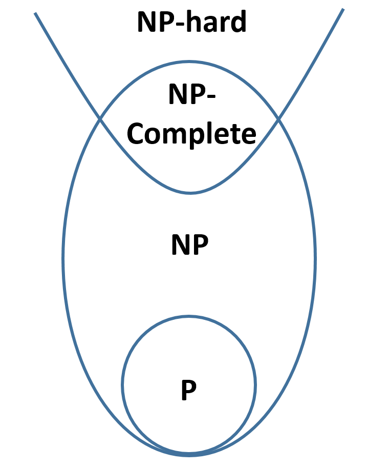
In this work, we start by surveying the use of dynamical systems in the context of constructing state-of-the-art algorithms for NP-hard problems. In particular, we will cover the use of dynamical systems theory for constructing decentralized graph clustering algorithms Cit:cluster1; Cit:cluster2, solutions for the TSP Cit:TSP_sahai, and quantum-inspired networks of Duffing oscillators for solving the MAX-CUT problem Cit:quantum_net. We then switch to the use of dynamical systems theory for analysis of algorithms Cit:koopman and the underlying problems Cit:zoltan; Cit:zoltan2.
The goal of this survey paper is to highlight the potential application of dynamical systems theory for optimization of complex functions and analysis of computational complexity theory. This is a nascent field which presents the possibility of tremendous impact. Additionally, we expect this area to lead to new theoretical developments in nonlinear dynamics theory and novel algorithms for computationally intractable problems.
Ziessler, Surana, Speranzon, Klus, Dellnitz, and Banaszuk have all served as co-authors in my efforts in this area. However, my extensive discussions with Prof. Michael Dellnitz inspired me to delve deeper into the area of dynamical systems and the analysis of algorithms!
2 Novel algorithm construction: decentralized graph clustering
Overview Algorithms for graph analysis have a wide variety of applications such as routing, pattern recognition, database searches, network layout, and Internet PageRank to name a few Cit:graph_algos. Although some of these problems can solved efficiently on present day computing devices, several graph analysis problems are computationally intractable Cit:cormen. For example, the problem of partitioning graphs into equal size sets while minimizing the weights of cut edges arises in a range of settings such as social anthropology, gene networks, protein sequences, sensor networks, computer graphics, and Internet routing algorithms Cit:cluster2. To avoid unbalanced cuts, size restrictions are typically placed on the clusters; instead of minimizing inter-connection strength, if one minimizes the ratio of the inter-connection strength to the size of individual clusters, the problem becomes NP-complete Cit:tutorial; Cit:npcomp.
In Cit:cluster1; Cit:cluster2, a novel decentralized algorithm for clustering/partitioning graphs that exploits fundamental properties of a dynamically evolving networked system was constructed. In particular, by propagating waves in a graph, one can compute partitions or clusters in a completely decentralized setting. The method is orders of magnitude faster than existing approaches Cit:kempe. This is our first example of a dynamical systems theory based algorithm for a combinatorial optimization problem. We now discuss the details of the approach. Let be a graph with vertex set and edge set , where a weight is associated with each edge , and is the weighted adjacency matrix of . We assume that if and only if . The (normalized) graph Laplacian is defined as,
| (1) |
or equivalently, where is the diagonal matrix with the row sums of .
Note that in Cit:cluster2, only undirected graphs were considered. The smallest eigenvalue of the Laplacian matrix is , with an associated eigenvector . Eigenvalues of can be ordered as, with associated eigenvectors Cit:tutorial. It is well known that the multiplicity of is the number of connected components in the graph Cit:tutorial.
Given the Laplacian matrix , associated with a graph , spectral clustering divides into two clusters by computing the signs of the elements of the second eigenvector , or Fiedler vector. For further details about the computation of two or more clusters see Cit:tutorial.
There are many algorithms to compute eigenvectors, such as the Lanczos method or orthogonal iteration GolubVanLoan96. Although some of these methods are distributable, convergence is slow GolubVanLoan96 and these algorithms do not consider/take advantage of the fact that the matrix for which the eigenvalues and eigenvectors need to be computed is the adjacency matrix of the underlying graph. In Cit:kempe, the authors propose an algorithm to compute the first largest eigenvectors (associated with the first eigenvalues with greatest absolute value)11 1 Note that in the case of spectral clustering we desire to compute the smallest eigenvectors of . The algorithm is still applicable if we consider the matrix . of a symmetric matrix. The algorithm in Cit:kempe emulates the behavior of orthogonal iteration using a decentralized process based on gossip algorithms or deterministic random walks on graphs. This approach can be slow as it converges after iterations Cit:kempe where where is the mixing time for the random walk on the graph and is the number of nodes.
This procedure is equivalent to evolving the discretized heat equation on the graph and can be demonstrated as follows. The heat equation is given by,
where is a function of time and space, is the partial derivative of with respect to time, and is the Laplace operator Cit:cluster2.
When the above equation is discretized on a graph one gets the following equation:
for . Here is the scalar value of on node at time and are the neighbors of node in the graph. The graph Laplacian is the discrete counterpart of the operator. The above iteration can be re-written, in matrix form, where . The solution of this iteration is,
| (2) |
where constants depend on the initial condition . It is interesting to note that in Eqn. 2, the dependence of the solution on higher eigenvectors and eigenvalues of the Laplacian decays with increasing iteration count. Thus, it is difficult to devise a fast and distributed method for clustering graphs based on the heat equation.
In Cit:cluster1; Cit:cluster2, a novel algorithm based on the idea of permanent excitation of the eigenvectors of using dynamical systems theory is constructed. In a theme similar to Mark Kac’s question “Can one hear the shape of a drum?” DrumShape, it was demonstrated that by evolving the wave equation in the graph, nodes can “hear” the eigenvectors of the graph Laplacian using only local information. Moreover, it was shown, both theoretically and on examples, that the wave equation based algorithm is orders of magnitude faster than random walk based approaches for graphs with large mixing times. The overall idea of the wave equation based approach is to simulate, in a distributed fashion, the propagation of a wave through the graph and capture the frequencies at which the graph “resonates”. In other words, it was shown that by using these frequencies one can compute the eigenvectors of the Laplacian, thus clustering the graph.
The wave equation based clustering approach can be described as follows. Analogous to the heat equation case (Eq. 2), the solution of the wave equation can be expanded in terms of the eigenvectors of the Laplacian. However, unlike the heat equation where the solution eventually converges to the first eigenvector of the Laplacian, in the wave equation all the eigenvectors remain eternally excited (a consequence of the second derivative of with respect to time). This observation is used to develop a simple, yet powerful, distributed eigenvector computation algorithm. The algorithm involves evolving the wave equation on the graph and then computing the eigenvectors using local FFTs. The graph decomposition/partitioning algorithm based on the discretized wave equation on the graph, given by
| (3) |
where originates from the discretization of the spatial derivatives in the wave equation. The rest of the terms originate from discretization of the term in the wave equation. To update using Eq. 3, one needs only the value of at neighboring nodes and the connecting edge weights (along with previous values of ).
The main steps of the algorithm are shown as Algorithm 1. Note that at each node (node in the algorithm) one only needs nearest neighbor weights and the scalar quantities also at nearest neighbors. We emphasize, again, that is a scalar quantity and Random() is a random initial condition on the interval . The vector is the -th component of the -th eigenvector, is a positive integer derived in Cit:cluster1; Cit:cluster2, FrequencyPeak(Y,j) returns the frequency at which the -th peak occurs and return the corresponding Fourier coefficient.
Proposition 1
The clusters of graph , determined by the signs of the elements of the eigenvectors of , can be computed using the frequencies and coefficients obtained from the Fast Fourier Transform of , for all and some . Here is governed by the wave equation on the graph (shown in Eqn. 3) with the initial condition and .
Proof
For the proofs see Cit:cluster1; Cit:cluster2.
The above proof demonstrates that the approach is fundamentally decentralized. Moreover, it is shown in Cit:cluster1; Cit:cluster2 that the convergence of the wave equation based eigenvector computation depends on the mixing time of the underlying Markov chain on the graph, and is given by,
| (4) |
where is the mixing time of the Markov chain. Thus, the wave equation based algorithm has better scaling with for graphs of any size (given by , see Fig. 2).
The above work is an example of the construction of a state-of-the-art algorithm using dynamical systems theory. This work has also found application in distributed numerical computations Cit:Num_klus and uncertainty quantification Cit:UQ_surana. We now present another example of constructing novel algorithms for NP-hard problems using the theory of nonlinear dynamics and invariant manifold computations.
3 Novel algorithm construction: invariant manifolds and the traveling salesman problem
Overview Recently, dynamical systems theory was used to construct novel algorithms for another iconic NP-hard problem Cit:TSP_sahai. The traveling salesman problem (TSP) has a long and rich history in the areas of computer science, optimization theory, and computational complexity, and has received decades of interest Cit:cook. This combinatorial optimization problem arises in a wide variety of applications related to genome map construction, telescope management, and drilling circuit boards. The TSP also naturally occurs in applications related to target tracking Cit:target_tracking, vehicle routing, and communication networks to name a few. We refer the reader to Cit:cook; Cit:TSP_sahai for further details.
In its basic form, the statement of the TSP is exceedingly simple. The task is to find the shortest Hamiltonian circuit through a list of cities, given their pairwise distances. Despite its simplistic appearance, the underlying problem is NP-hard Cit:karp. Several heuristics have been developed over the years to solve the problem Cit:cook including ant colony optimization, cutting plane methods, Christofides heuristic algorithm, and the Lin–Kernighan heuristic.
In Cit:TSP_sahai, inspired by dynamical systems theory, the authors construct novel orthogonal relaxation based approximations to the TSP. In particular, the constructed dynamical system captures the flow on the manifold of orthogonal matrices and ideally converges to a permutation matrix that minimizes the tour length. However, in general, the flow typically converges to local minima that are not competitive when compared to state-of-the-art heuristics. Inspired by this continuous relaxation, the authors compute the solution to a two-sided orthogonal Procrustes problem Cit:Procrustes-book that relaxes the TSP to the manifold of orthogonal matrices. They then combine the Procrustes approach with the Lin–Kernighan heuristic Cit:LKH for computing solutions of the TSP. Additionally, the authors use set-oriented methods to study the stability of optimal solutions and their stable manifolds, thereby providing insight into the associated basins of attraction and the resulting computational complexity of the problem.
Given a list of cities and the associated distances between cities and , denoted by , the TSP aims to find an ordering of such that the tour cost, given by
| (5) |
is minimized. For the Euclidean TSP, for instance, , where is the position of . In general, however, the distance matrix does not have to be symmetric (for example see Cit:tsp_asymm). The ordering can be represented as a unique permutation matrix . Note, however, that due to the underlying cyclic symmetry, multiple orderings – corresponding to different permutation matrices – have the same cost.
There are several equivalent ways to define the cost function of the TSP. The authors restrict themselves to the trace22 2 The trace of a matrix is defined to be the sum of all diagonal entries, i.e., . formulation. Let denote the set of all permutation matrices, then the TSP can be written as a combinatorial optimization problem of the form
| (6) |
where and . Here, is defined to be the adjacency matrix of the cycle graph of length .
One uses the undirected cycle graph adjacency matrix for symmetric TSPs and the one corresponding to the directed cycle graphs for asymmetric TSPs. The matrices are defined as,
The work in Cit:TSP_sahai focuses on the undirected version of the TSP. By relaxing the TSP problem to the manifold of orthogonal matrices (since permutation matrices are orthogonal matrices restricted to or entries), one can use the two sided Procrustes problem to solve the problem exactly, as outlined in the theorem below.
Theorem 3.1
Given two symmetric matrices and , whose eigenvalues are distinct, let and be eigendecompositions, with , , and as well as . Then every orthogonal matrix which minimizes
| (7) |
has the form
where .
A proof of this theorem can be found in Cit:Sch68. If the eigenvalues of and are distinct, then there exist different solutions with the same cost. If one or both of the matrices possess repeated eigenvalues, then the eigenvectors in the matrices and are determined only up to basis rotations, which further increases the size of the solution space. The Procrustes problem is related to a dynamical system formulation of the TSP as outlined below.
The orthogonal relaxation of the combinatorial optimization problem (6), given by (7), can be solved using a steepest descent method on the manifold of orthogonal matrices. For more details about this formulation see Cit:TSP_sahai. One can pose the TSP as a constrained optimization problem of the form,
| (8) | ||||
| (9) |
This formulation gives rise to the following set of equations,
| (10) | ||||
The above set of equations are obtained by using gradient descent on the Lagrangian cost function.
Example 1
In order to illustrate the gradient flow approach, let us consider a simple TSP with 10 cities. Using (10), we obtain the results shown in Figure 3. In this example, the dynamical system converges to the optimal tour.


The dynamical system without constraints converges to equilibria that are given by the Procrustes solutions. To shed light on the stability and local dynamics around the optimal TSP solutions one can approximate subsets of the stable manifold of the Procrustes solutions such that two permutation matrices are inside these sets. This numerical study enables the analysis of the robustness of Procrustes solutions under small perturbations of the initial permutation matrix and the assessment of the ‘closeness’ the Procrustes solution is to the optimal permutation matrix. In order to compute the sets of interest, set-oriented continuation techniques developed in DH96 are used in Cit:TSP_sahai. An example computation is depicted in Fig. 4.

Moreover, one can also use set oriented methods to compute basins of attraction of optimal permutation matrices for small instances of the TSP. These basins (subsets of the stable manifold) are computed by perturbing the optimal solutions and integrating the flow backward in time Cit:TSP_sahai. The solutions are shown in Fig. 5. These computations are interesting and capture the “hardness” of the problem. In particular, one can see that the solutions of relaxed versions of the problem (such as the relaxations to the manifolds of orthogonal matrices) do not, in general, lie in the basin of attraction of the optimal solutions of the original problem. Other such instances of analysis of relaxed solutions of the TSP using dynamical systems theory are outlined in Cit:TSP_sahai.

(a)

(b)
Although, dynamical systems theory demonstrates that the Procrustes solutions do not typically lie in the basin of attraction of the optimal solutions of the TSP, a new biasing scheme for the Lin–Kernighan heuristic is constructed using the aforementioned relaxation Cit:TSP_sahai.
The Lin–Kernighan heuristic is a popular heuristic for the TSP Cit:LKH. Starting from an initial tour, the approach progresses by extracting edges from the tour and replacing them with new edges, while maintaining the Hamiltonian cycle constraint. If edges in the tour are simultaneously replaced, this is known as the -opt move Cit:LKH. To prune the search space, the algorithm relies on minimum spanning trees to identify edges that are more likely to be in the tour. This “importance” metric for edges is called -nearness and described in Cit:LKH; Cit:TSP_sahai. The algorithm has found great success on large instances of the TSP, see Cit:cook for more details.
In Cit:TSP_sahai, the -nearness metric is replaced with a new Procrustes solution–based metric that prunes/identifies important potential edges to include in the “candidate set list”. This list is then used to generate the -opt moves. The metric is captured in Fig. 6. The Procrustes solution tends to capture the longer edges that are important. To increase the inclusion of the short edges, the approach in Cit:TSP_sahai constructs a homotopy between the Procrustes (-nearness) solution and the distance matrix. Using a graph Laplacian approach, the mixture of the two matrices is compared to the -nearness approach on 22 well-known instances of the TSP. -nearness based LKH converges to lower cost values in of the instances when compared to -nearness based LKH. Moreover, for random TSP instances of size (cities) it is found that -nearness has lower tour costs after a fixed number of -opt moves in of the instances, translating into an improvement for of the instances.

Thus, this is another example that demonstrates that dynamical systems theory can be used to analyze NP-hard problems and construct improved heuristics.
We now show how networks of Duffing oscillators can be used to construct a new algorithm for the iconic MAX-CUT problem.
4 Novel algorithm construction: network of Duffing oscillators for the MAX-CUT problem
Overview MAX-CUT Cit:karp is a well-known NP-hard problem that arises in graph theory. Simply stated, the goal is to compute a subset of the vertex set in a graph , such that the number of edges between and the rest of the graph are maximized. The best known approximation ratio of can be achieved in polynomial time using semi-definite programming Cit:Goemans. The problem naturally arises in VLSI design and statistical physics, and has been extensively studied.
In Cit:quantum_net, the authors construct an optimization algorithm by simulating the adiabatic evolution of Hamiltonian systems which can be used to approximate the MAX-CUT solution of an all-to-all connected graph. The approach is inspired by quantum adiabatic optimization for Ising systems Cit:Ising with the following energy,
| (11) |
where are the spins which can take values {-1,1} and is the coupling coefficient. Finding the lowest energy state of the Ising system is computationally challenging (for a system with N spins, the potential number of states is ). Note that one can map the Ising problem to the MAX-CUT problem by setting , where is the weight of the edge that connects nodes and . It is easy to show that minimizing the energy in Eqn. 11 corresponds computing the solution of the MAX-CUT problem.
The approach outlined in Cit:quantum_net relies on the adiabatic evolution of a network of nonlinear oscillators. This system exhibits a bifurcation (called “simulated bifurcation”) for each nonlinear oscillator. The two branches correspond to the and values for each spin. The authors exploit Graphical Processing Units (GPU) and Field Programmable Gate Array (FPGA) platforms to compute the solution of these Hamiltonian systems. This method is compared to existing methods and displays orders-of-magnitude improvement. The approach is demonstrated on an Ising system with 100,000 spins. Consider the Hamiltonian that arises in Kerr-nonlinear parametric oscillators,
| (12) |
Here and are position and momentum of the -th oscillator respectively, is the Kerr coefficient, is the parametric pumping amplitude, and is the detuning frequency between the natural frequency of the -th oscillator and half the pumping frequency. Using the standard Hamiltonian formulation, one can derive equations of motion for each oscillator. Evolving these system of equations for and converges to low energy solutions of an Ising system (Eqn. 11) with high probability. Thus, the sign of at the end of the simulation determines the -th spin. However, the above equations are computationally challenging to simulate from a numerical perspective.
Instead of using the equations that arise from the “full” Hamiltonian in Eqn. 12, the authors (in Cit:quantum_net) construct a simplified Hamiltonian of the form,
| (13) |
The above Hamiltonian corresponds to the following system of equations,
| (14) |
It is easy to see that the above system of equations are a network of Duffing oscillators Cit:Gucken. The separability of the Hamiltonian (Eqn. 13) makes the numerical integration of the system of equations easier. In particular, the authors use an explicit symplectic Euler scheme which makes it amenable for one to hard wire the resulting computational circuits on an FPGA platform. The computation proceeds as follows: all and variables are initially set to zero, is then increased from and the system in Eqn. 14 is evolved. The sign of the final value of serves as an approximation of the -th spin of the associated Ising system.
The system in Eqn. 14 has two branches of solutions as is increased from zero. It is easy to see that these branches correspond to for each oscillator and, consequently, leads to a solution space. If one varies slowly, the adiabatic theorem ensures that if one converges to a low energy solution for close to , the final solutions (for large ) will also correspond to low energy.
This method is compared to state-of-the-art approaches for two instances of the MAX-CUT problem. In the first instance, an all-to-all 2000 node MAX-CUT problem is solved on an FPGA using the above approach. The authors demonstrate that the above framework successfully converges to the best known solutions Cit:Goemans very quickly. Moreover, they test the approach on a 100,000 size problem (with edges) and find that their approach converges to the answer times faster than existing software on GPU hardware. For more details of the work and associated results we refer the reader to Cit:quantum_net.
Thus far, we have summarized three examples in which dynamical systems theory was used to construct novel algorithms for NP-hard problems. We now discuss approaches that exploit nonlinear dynamics theory to analyze optimization algorithms for NP-hard problems.
5 Analysis of algorithms: Koopman operators based analysis of algorithms
Overview Koopman operator theory is one of the most active and exciting sub-areas within dynamical systems theory Cit:koop_mez; Cit:koop_klus; Cit:koop_kev; Cit:koop_kutz. The approach is based on the construction of an infinite dimensional linear operator that captures the evolution of the observables of the underlying nonlinear system. Consequently, the spectra and eigenfunctions of the operator, capture system dynamics. This methodology has been used used in a wide variety of settings, including system control and identification. An advantage of Koopman operator based methodologies is that the computations are typically based on time trace data of system evolution Cit:DMD. In recent work Cit:koopman, Koopman operator theory was used to analyze algorithms. In particular, the authors consider optimization algorithms that evolve their state in the form of iterations. An assumption is made that the algorithm state spaces are smooth -dimensional Riemannian submanifolds in -dimensional Euclidean spaces. A single iteration of the state is represented as,
| (15) |
where is the iteration count. These iterative algorithms can sometimes be represented in continuous form (akin to the process used in Cit:Nesterov). In other words, one can (in the limit) represent the algorithm as a continuous vector field . If one starts at an initial condition , the continuous time representation is of the form Cit:koopman,
| (16) |
As shown in Cit:koopman, this continuous form can be approximated using a Koopman operator framework. The authors then use this approach to study gradient descent and Newton-Raphson from a global dynamics perspective. Although the examples fall under the category of continuous optimization, the approach can certainly be used to study combinatorial optimization algorithms in the future. Using the same nomenclature as in Cit:koopman, consider a dynamical system of the form,
| (17) |
then the family of Koopman operators acts on the function space of observables as follows,
| (18) |
An function space with an inner product is typically chosen for the space of observables. For more details, on the approach and choice of function space see Cit:koopman. Note that the Koopman operator is the adjoint of the Perron-Frobenius operator Cit:Perron_Frob. Letting , without loss of generality, The Koopman operator can be expanded in terms of its spectrum,
| (19) |
where lie in the discrete part and is the continuous spectrum of the operator. and are projection operators for their corresponding eigenspaces. The eigenfunctions of the Koopman operator are,
| (20) |
Thus, one can predict the evolution of observables,
| (21) |
The operator can be numerically approximated using a data driven approach as outlined in Cit:koop_kev; Cit:koop_kutz. The popular extended dynamic mode decomposition (EDMD) methodology introduced in Cit:koop_kev is used to analyze algorithms using the Koopman operator lens Cit:koopman.
The EDMD approach approximates the action of the infinite dimensional operator using a finite set of real-valued functions (also called “dictionary”). In particular, given a smooth manifold sampled by a finite set of points , the EDMD approach computes the action of the Koopman operator on the dictionary of points in . The operator itself is approximated using a least squares approach Cit:koop_kev as outlined below. Given a dictionary of observables one can define a matrix of the form . Then the Koopman operator can be approximated as,
| (22) |
where is the size of the dataset and . For more details see Cit:koop_kev.
The operator gives a local approximation of the underlying algorithm applied to a specific instance of a problem. In particular, one can use the data of a short burst of computation to compute a local approximation of the dynamics of the algorithm to accelerate its convergence. The eigenvalues, vectors, and modes are computed using EDMD. This approximation is used as a data-driven surrogate for the system to accelerate optimization. In Cit:koopman, the authors use the following cost function,
| (23) |
to demonstrate utility of the Koopman approach. The function has one local maximum and four local minima Cit:koopman. The authors study the the popular gradient descent algorithm using the Koopman operator framework. In particular, they use radial basis functions to form a dictionary and compute eigenvalues and eigenfunctions. They show that one can construct an ergodic decomposition of the state space, thereby separating the different basins of attraction Cit:koopman. The approach is able to capture the global dynamics of the algorithm in this setting, providing valuable insight regarding the performance and limitations of the algorithm.
Additionally, the authors demonstrate the use of Koopman operators for studying global dynamics of algorithms in high-dimensional spaces. They take the example of a -dimensional problem and show that the dynamics quickly contracts to a low dimensional subset. They demonstrate that one can accelerate the prediction of trajectories of gradient descent with high accuracy. The work concludes with the illustration of the utility of Koopman operators for analyzing the iconic Newton-Raphson method for root finding Cit:koopman. For a complex polynomial of degree two, they show that the eigenfunction diverges at the roots. They also show that in cases of chaotic behavior of Newton-Raphson, one can use approximations Cit:Mezic_cont of the continuous spectrum of the Koopman operator to study statistical properties of the emergent chaos.
Although the above Koopman methodology was demonstrated on problems of continuous optimization, it provides a new technique with which one can study combinatorial optimization problems. We anticipate that the Koopman operator approach will be a new tool with which to study algorithms for NP-hard problems and improve their performance.
6 Analysis of algorithms: Chaos and dynamical systems for analyzing the satisfiability (SAT) problem
Overview The satisfiability problem is another iconic problem that frequently arises in the study of computational complexity theory. The challenge here is to find a satisfying assignment for a logical formula. In particular, a -SAT Boolean formula of Boolean variables and clauses, , is written in the conjunctive normal form (CNF) biere2009handbook as follows,
| (24) |
where is the literal in clause . A SAT formula is said to be satisfiable if there exists an assignment for the binary variables such that . It is well known that the satisfiability problem is NP-complete Cit:cook. A critical parameter associated with the satisfiability problem is the clause density biere2009handbook. In particular, the probability that a random -SAT instance is satisfiable undergoes a phase transition as a function of () biere2009handbook. The MAX-SAT problem (and the corresponding weighted version) krentel1988complexity requires one to find that assignment (or assignments) that maximize the number (or the cumulative weights) of satisfied clauses. Consider a SAT formula , then every assignment can be mapped to an “energy” such that,
| (25) |
where , if the -th clause evaluates to true. In other words, the goal under the MAX-SAT problem is to find the assignment for such that the number of satisfied clauses (or energy) is maximized. The MAX-SAT problem is harder (from a computational standpoint) than the SAT problem. In particular, it is known to be strongly NP-hard (there are no polynomial time approximation schemes). The problem of computing density of states (DOS) encompasses the the SAT and MAX-SAT problems. Classical and quantum algorithms for estimating the DOS of logical formulae were constructed in Cit:SAT_sahai.
In a series of seminal papers Cit:zoltan; Cit:zoltan2; Cit:zoltan3, the authors construct a dynamical systems approach to study satisfiability problems. They construct a dynamical system that computes the solutions of SAT instances. Here, the equilibria of the dynamical system correspond to literal values for which the SAT formula in Eqn. 24 evaluates to true. They prove that the dynamical system admits no false equilibria or limit cycles. Additionally, they relate the emergence of transient chaos and fractal boundaries with optimization hardness of the problem instance Cit:zoltan, pointing to a deep connection between dynamical systems theory and computational complexity. As mentioned in the overview, in Cit:zoltan, the authors embed SAT equations into a system of ordinary differential equations using the the following mapping: let , i.e. can take values between and such that,
Generalizing the dynamical system for satisfiability problems constructed in Cit:zoltan, one can define and as follows,
Note that , if and only if -th clause is satisfied i.e. for at least one variable that appears in clause . In Cit:zoltan, the authors define an energy function of the form such that only at a solution of the satisfiability problem. The auxiliary variables prevent the non-solution attractors from trapping the search dynamics (for more information see Cit:zoltan).
In Cit:zoltan, the authors find that as the constraint density of the k-SAT problem increases, the trajectories of the dynamical system display intermittent chaos with fractal basin boundaries Cit:zoltan. Note that, in this work, the existence of chaos is associated with the emergence of positive finite size Lyapunov exponents (FSLE) Cit:gucken and the emergence of chaos corresponds to the well known phase transitions in the -SAT problem Cit:zoltan.
In Cit:zoltan2, the authors further exploit the above system of equations to study the -SAT problem with increasing constraint density. They find that hardness appears as a second order phase transition and discover that the resulting transient chaos displays a novel exponential-algebraic scaling. In Cit:zoltan3, the authors exploit the above framework to construct novel solvers for the MAX-SAT problem. This body of work demonstrates that dynamical systems theory can, in fact, be used to simultaneously study computational complexity theory and construct novel algorithms for NP-hard problems.
7 Conclusion
Combinatorial optimization is a wide and important area of research with numerous applications. For decades, computer scientists have developed novel algorithms for addressing these problems. Some problems are amenable to algorithms and theory developed thus far (examples include graph routing and sorting), while others, in general, remain intractable from a computational standpoint (such as the traveling salesman problem and MAX-SAT) despite significant efforts. The classification of problems into different classes (such as NP, NP-hard, and PSPACE) and associated analyses has given rise to the field of computational complexity theory.
Nonlinear dynamics, on the other hand, arises in a multitude of engineering and scientific settings. The theory has been used to explain system behavior in a diverse set of fields such as fluidics, structural mechanics, population dynamics, epidemiology, optics, and aerospace propulsion. However, the application of the theory of dynamical systems to combinatorial optimization and computational complexity remains limited.
In this survey article, we summarize five recent examples of using dynamical systems theory for constructing and analyzing combinatorial optimization problems. In particular, we cover a) a novel approach for clustering graphs using the wave equation partial differential equation (PDE), b) invariant manifold computations for the traveling salesman problem, c) novel approaches for building quantum networks of Duffing oscillators to solve the MAX-CUT problem, d) applications of the Koopman operator for analyzing optimization algorithms, and e) the use of dynamical systems theory to analyze computational complexity of the SAT problem.
We note that the above set of examples are not comprehensive and there are several examples that have been omitted in this survey. However, the goal of this article is not to provide a complete list of all such examples but to demonstrate that dynamical systems theory can be exploited to construct algorithms and approaches for optimization problems. Even more importantly, we hope to inspire others to extend existing dynamical systems approaches to construct the next-generation of techniques and insights for combinatorial optimization.
Acknowledgements.
This material is based upon work supported by the Defense Advanced Research Projects Agency (DARPA) and Space and Naval Warfare Systems Center, Pacific (SSC Pacific) under Contract No. N6600118C4031.References
- (1) Poincaré, H.: Sur le problème des trois corps et les équations de la dynamique. Acta Mathematica 13, A3–A270 (1890)
- (2) Turing, A.: On computable problems with an application to the entscheidungsproblem. Proc. London Math. Society 2, 42 (1936)
- (3) Church, A.: A set of postulates for the foundation of logic. Annals of mathematics, 346–366 (1932)
- (4) Strogatz, S. H.: Nonlinear dynamics and chaos: with applications to physics, biology, chemistry, and engineering. CRC press (2018).
- (5) Walleczek, J. (Ed.): Self-organized biological dynamics and nonlinear control: toward understanding complexity, chaos and emergent function in living systems. Cambridge University Press (2006).
- (6) Kevrekidis, I. G., Schmidt, L. D., and Aris, R.: On the dynamics of periodically forced chemical reactors. Chemical engineering communications, 30(6), 323-330 (1984).
- (7) Holmes, P., Lumley, J. L., Berkooz, G., and Rowley, C. W. (2012). Turbulence, coherent structures, dynamical systems and symmetry. Cambridge University Press.
- (8) Liu, W. M., Hethcote, H. W., and Levin, S. A.: Dynamical behavior of epidemiological models with nonlinear incidence rates. Journal of mathematical biology, 25(4), 359-380 (1987).
- (9) Dellnitz, M. and Junge, O. Set oriented numerical methods for dynamical systems. Handbook of dynamical systems, 2, 221-264 (2002).
- (10) Mezić, I. Analysis of fluid flows via spectral properties of the Koopman operator. Annual Review of Fluid Mechanics, 45, 357-378 (2013).
- (11) Hummer, G. and Kevrekidis, I. G. Coarse molecular dynamics of a peptide fragment: Free energy, kinetics, and long-time dynamics computations. The Journal of chemical physics, 118(23), 10762-10773 (2003).
- (12) Hasselblatt, B. and Katok, A. (Eds.). Handbook of dynamical systems. Elsevier (2002).
- (13) Lorenz, E. N. Deterministic nonperiodic flow. Journal of the atmospheric sciences, 20(2), 130-141 (1963).
- (14) Morse, M. and Hedlund, G. A. Symbolic dynamics. American Journal of Mathematics, 60(4), 815-866 (1938).
- (15) Guckenheimer, J., and Holmes, P. (2013). Nonlinear oscillations, dynamical systems, and bifurcations of vector fields (Vol. 42). Springer Science & Business Media.
- (16) Nesterov, Y. A method for unconstrained convex minimization problem with the rate of convergence . In Doklady an ussr (Vol. 269, pp. 543-547) (1983).
- (17) Su, W., Boyd, S., and Candes, E. A differential equation for modeling Nesterov’s accelerated gradient method: Theory and insights. In Advances in Neural Information Processing Systems (pp. 2510-2518) (2014).
- (18) Wibisono, A., Wilson, A. C., and Jordan, M. I. A variational perspective on accelerated methods in optimization. Proceedings of the National Academy of Sciences, 113(47), E7351-E7358 (2016).
- (19) Cook, S. A. The complexity of theorem-proving procedures. In Proceedings of the third annual ACM Symposium on Theory of Computing, 151-158 (1971).
- (20) Karp, R. M. Reducibility among combinatorial problems. In Complexity of computer computations, 85-103. Springer, Boston, MA (1972).
- (21) Lin, S. Computer solutions of the traveling salesman problem. Bell System Technical Journal, 44(10), 2245-2269 (1965).
- (22) Cook, W. J. In pursuit of the traveling salesman: Mathematics at the limits of computation. Princeton University Press (2011).
- (23) Peikert, C. A decade of lattice cryptography. Foundations and Trends® in Theoretical Computer Science, 10(4), 283-424 (2016).
- (24) Klus, S., and Sahai, T. A spectral assignment approach for the graph isomorphism problem. Information and Inference: A Journal of the IMA, 7(4), 689-706 (2018).
- (25) Helsgaun, K. An effective implementation of the Lin–Kernighan traveling salesman heuristic. European Journal of Operational Research, 126(1), 106-130 (2000).
- (26) Applegate, D., Bixby, R., Chvatal, V., and Cook, W. Concorde TSP solver (2006).
- (27) Sahai, T., Speranzon, A., and Banaszuk, A. Wave equation based algorithm for distributed eigenvector computation. In 49th IEEE Conference on Decision and Control (CDC) (pp. 7308-7315) (2010, December).
- (28) Sahai, T., Speranzon, A., and Banaszuk, A. Hearing the clusters of a graph: A distributed algorithm. Automatica, 48(1), 15-24 (2012).
- (29) Sahai, T., Ziessler, A., Klus, S., and Dellnitz, M. Continuous relaxations for the traveling salesman problem. Nonlinear Dynamics, 97(4), 2003-2022 (2019).
- (30) Goto, H., Tatsumura, K., and Dixon, A. R. Combinatorial optimization by simulating adiabatic bifurcations in nonlinear Hamiltonian systems. Science Advances, 5(4), eaav2372 (2019).
- (31) Dietrich, F., Thiem, T. N., and Kevrekidis, I. G. On the Koopman operator of algorithms. arXiv preprint arXiv:1907.10807 (2019).
- (32) Ercsey-Ravasz, M. and Toroczkai, Z. Optimization hardness as transient chaos in an analog approach to constraint satisfaction. Nature Physics, 7(12), 966-970 (2011).
- (33) Varga, M., Sumi, R., Toroczkai, Z., and Ercsey-Ravasz, M. Order-to-chaos transition in the hardness of random Boolean satisfiability problems. Physical Review E, 93(5), 052211 (2016).
- (34) Even, S. Graph algorithms. Cambridge University Press (2011).
- (35) Cormen, T. H., Leiserson, C. E., Rivest, R. L., and Stein, C. Introduction to algorithms. MIT press (2009).
- (36) Von Luxburg, U. A tutorial on spectral clustering. Statistics and computing, 17(4), 395-416 (2007).
- (37) Wagner, D. and Wagner, F. Between min cut and graph bisection. In International Symposium on Mathematical Foundations of Computer Science (pp. 744-750). Springer, Berlin, Heidelberg (1993, August).
- (38) Golub, G. H. and Van Loan, C. F. Matrix Computations Johns Hopkins University Press. Baltimore and London (1996).
- (39) Kempe, D. and McSherry, F. A decentralized algorithm for spectral analysis. Journal of Computer and System Sciences, 74(1), 70-83 (2008).
- (40) Kac, M. Can one hear the shape of a drum?. The American Mathematical Monthly, 73(4P2), 1-23 (1966).
- (41) Klus, S., Sahai, T., Liu, C., and Dellnitz, M. An efficient algorithm for the parallel solution of high-dimensional differential equations. Journal of computational and applied mathematics, 235(9), 3053-3062 (2011).
- (42) Surana, A., Sahai, T., and Banaszuk, A. Iterative methods for scalable uncertainty quantification in complex networks. International Journal for Uncertainty Quantification, 2(4) (2012).
- (43) Englot, B., Sahai, T., and Cohen, I. Efficient tracking and pursuit of moving targets by heuristic solution of the traveling salesman problem. In 52nd IEEE Conference on Decision and Control (pp. 3433-3438). IEEE (2013, December).
- (44) J.C. Gower and G.B. Dijksterhuis. Procrustes problems, volume 3. Oxford University Press New York (2004).
- (45) Sahai, T., Klus, S., and Dellnitz, M. A Traveling Salesman Learns Bayesian Networks. arXiv preprint arXiv:1211.4888 (2012).
- (46) Schönemann, P. H. On two-sided orthogonal Procrustes problems. Psychometrika, 33(1), 19-33 (1968).
- (47) Dellnitz, M. and Hohmann, A. The computation of unstable manifolds using subdivision and continuation. In Nonlinear dynamical systems and chaos (pp. 449-459). Birkhäuser, Basel (1996).
- (48) Goemans, M. X., and Williamson, D. P. Improved approximation algorithms for maximum cut and satisfiability problems using semidefinite programming. Journal of the ACM (JACM), 42(6), 1115-1145 (1995).
- (49) Glauber, R. J. Time-dependent statistics of the Ising model. Journal of mathematical physics, 4(2), 294-307 (1963).
- (50) Guckenheimer, J. and Holmes, P. Nonlinear oscillations, dynamical systems, and bifurcations of vector fields (Vol. 42). Springer Science & Business Media (2013).
- (51) Budisić, M., Mohr, R., and Mezić, I. Applied Koopmanism. Chaos: An Interdisciplinary Journal of Nonlinear Science, 22(4), 047510 (2012).
- (52) Klus, S., Koltai, P., and Schütte, C. On the numerical approximation of the Perron-Frobenius and Koopman operator. arXiv preprint arXiv:1512.05997 (2015).
- (53) Williams, M. O., Kevrekidis, I. G., and Rowley, C. W. A data–driven approximation of the Koopman operator: Extending dynamic mode decomposition. Journal of Nonlinear Science, 25(6), 1307-1346 (2015).
- (54) Lusch, B., Kutz, J. N., and Brunton, S. L. Deep learning for universal linear embeddings of nonlinear dynamics. Nature communications, 9(1), 1-10 (2018).
- (55) Kutz, J. N., Brunton, S. L., Brunton, B. W., and Proctor, J. L. Dynamic mode decomposition: data-driven modeling of complex systems. Society for Industrial and Applied Mathematics (2016).
- (56) Dellnitz, M., Hohmann, A., Junge, O., and Rumpf, M. Exploring invariant sets and invariant measures. Chaos: An Interdisciplinary Journal of Nonlinear Science, 7(2), 221-228 (1997).
- (57) Korda, M., Putinar, M., and Mezić, I. Data-driven spectral analysis of the Koopman operator. Applied and Computational Harmonic Analysis (2018).
- (58) Molnár, B., Molnár, F., Varga, M., Toroczkai, Z., and Ercsey-Ravasz, M. A continuous-time MaxSAT solver with high analog performance. Nature communications, 9(1), 1-12 (2018).
- (59) Biere, A., Heule, M., and van Maaren, H. (Eds.). Handbook of satisfiability (Vol. 185). IOS press (2009).
- (60) Krentel, M. W. The complexity of optimization functions. Journal of Computer and System Sciences, 36(490-509), 10-1016 (1988).
- (61) Sahai, T., Mishra, A., Pasini, J. M., and Jha., S. Estimating the Density of States of Boolean Satisfiability Problems on Classical and Quantum Computing Platforms. 34th AAAI Conference on Artificial Intelligence (AAAI) 2020.