Exponential integrators for the stochastic Manakov equation

André Berg Address: Department of Mathematics and Mathematical Statistics, Umeå University, 90187 Umeå, Sweden Email address: andre.berglund@umu.se , David Cohen Address: Department of Mathematics and Mathematical Statistics, Umeå University, 90187 Umeå, Sweden and
Department of Mathematical Sciences, Chalmers University of Technology and University of Gothenburg, 41296 Gothenburg, Sweden Email address: david.cohen@chalmers.se and Guillaume Dujardin Address: Inria Lille Nord-Europe and Laboratoire Paul Painlevé UMR CNRS 8524,
59650 Villeneuve d’Asq Cedex, France Email address: guillaume.dujardin@inria.fr

Abstract.

This article presents and analyses an exponential integrator for the stochastic Manakov equation, a system arising in the study of pulse propagation in randomly birefringent optical fibers. We first prove that the strong order of the numerical approximation is $1/2$ if the nonlinear term in the system is globally Lipschitz-continuous. Then, we use this fact to prove that the exponential integrator has convergence order $1/2$ in probability and almost sure order $1/2$ , in the case of the cubic nonlinear coupling which is relevant in optical fibers. Finally, we present several numerical experiments in order to support our theoretical findings and to illustrate the efficiency of the exponential integrator as well as a modified version of it. Stochastic partial differential equations. Stochastic Manakov equation. Coupled system of nonlinear Schrödinger equations. Numerical schemes. Exponential integrators. Strong convergence. Convergence in probability. Almost sure convergence. Convergence rates.

AMS Classification. 65C30. 65C50. 65J08. 60H15. 60M15. 60-08. 35Q55

1. Introduction

Optical fibers play an important role in our modern communication society [1]. In order to model the light propagation over long distance in randomly varying birefringent optical fibers, the Manakov PMD equation was derived from Maxwell’s equations in [25]. As noted in [16], polarization mode dispersion (PMD) is one of the main limiting effects of high bit rate transmission in optical fiber links. In addition, the work [16] proves that the asymptotic dynamics of the Manakov PMD equation is given by a stochastic nonlinear evolution equation in the Stratonovich sense: the stochastic Manakov equation, see below. In the present article, we perform a numerical analysis of this stochastic partial differential equation (SPDE).

We now review the literature on the numerical analysis of the stochastic Manakov equation. The work [18], see also [17], numerically studies the impact of noise on Manakov solitons and soliton wave-train propagation by the following time integrators: the nonlinearly implicit Crank–Nicolson scheme, the linearly implicit relaxation scheme, and a Fourier split-step scheme. For instance, it is conjectured that, in the small-noise regime and over short distances, solitons are not strongly destroyed and are stable. Reference [19], see also [17], proves that the order of convergence in probability of the Crank–Nicolson scheme is $1/2$ . On top of that, it is shown that this numerical integrator preserves the ${\mathbb{L}}^{2}$ -norm as does the exact solution to the stochastic Manakov equation. Furthermore, it is numerically observed that the almost-sure order of convergence of the relaxation scheme and the split-step scheme is $1/2$ .

The main goal of this article is to present and analyse a linearly implicit exponential integrator for the time discretisation of the stochastic Manakov equation. Exponential integrators for the time integration of deterministic or stochastic (partial) differential equations are nowadays widely used and studied as witnessed by the recent works [8, 15, 22, 21, 10, 23, 11, 26, 12, 3, 9, 2, 4, 7] and references therein. Beside having the same orders of convergence as the nonlinearly implicit Crank–Nicolson scheme from [19], the proposed exponential integrators offer additional computational advantages as illustrated below.

2. Setting and notation

Let $(\Omega,\mathcal{F},\mathbb{P})$ be a probability space on which a three-dimensional standard Brownian motion $W(t):=(W_{1}(t),W_{2}(t),W_{3}(t))$ is defined. We endow the probability space with the complete filtration $\mathcal{F}_{t}$ generated by $W(t)$ . In the present paper, we consider the nonlinear stochastic Manakov system [19]

(1)

i{\rm d}X+\partial^{2}_{x}X\,{\rm d}t+|X|^{2}X\,{\rm d}t+i\sqrt{\gamma}\sum_{k=1}^{3}\sigma_{k}\partial_{x}X\circ{\rm d}W_{k}=0,

where $X=X(t,x)=(X^{1},X^{2})$ is the unknown function with values in ${\mathbb{C}}^{2}$ with $t\geq 0$ and $x\in{\mathbb{R}}$ , the symbol $\circ$ denotes the Stratonovich product, $\gamma\geq 0$ measures the intensity of the noise, $|X|^{2}=|X^{1}|^{2}+|X^{2}|^{2}$ is the nonlinear coupling, and $\sigma_{1}$ , $\sigma_{2}$ and $\sigma_{3}$ are the classical Pauli matrices defined by

\sigma_{1}=\begin{pmatrix}0&1\\ 1&0\end{pmatrix},\hskip 18.49988pt\sigma_{2}=\begin{pmatrix}0&-i\\ i&0\end{pmatrix},\hskip 9.24994pt{\rm and}\hskip 9.24994pt\sigma_{3}=\begin{pmatrix}1&0\\ 0&-1\end{pmatrix}.

The mild form of the stochastic Manakov equation reads

(2)

X(t)=U(t,0)X^{0}+i\int_{0}^{t}U(t,s)F(X(s))\,\text{d}s,

where $X^{0}$ denotes the initial value of the problem, $U(t,s)$ for $t\geq s$ with $s,t\in{\mathbb{R}}_{+}$ is the random unitary propagator defined as the unique solution to the linear part of (1), and $F(X)=|X|^{2}X$ .

Let $p\geq 1$ . We define ${\mathbb{L}}^{p}:={\mathbb{L}}^{p}({\mathbb{R}}):=(L^{p}({\mathbb{R}};{\mathbb{C}}))^{2}$ the Lebesgue spaces of functions with values in ${\mathbb{C}}^{2}$ . We equip ${\mathbb{L}}^{2}$ with the real scalar product $\displaystyle(u,v)_{2}=\sum_{j=1}^{2}\mathrm{Re}\left(\int_{\mathbb{R}}u_{j}\overline{v}_{j}\,\text{d}x\right)$ . Further, for $m\in{\mathbb{N}}$ , we denote ${\mathbb{H}}^{m}:={\mathbb{H}}^{m}({\mathbb{R}})$ the space of functions in ${\mathbb{L}}^{2}$ with their $m$ first derivatives in ${\mathbb{L}}^{2}$ . The norm in ${\mathbb{H}}^{m}$ is denoted by $\left\lVert\cdot\right\rVert_{m}=\left\lVert\cdot\right\rVert_{{\mathbb{H}}^{m}}=\left\lVert\cdot\right\rVert_{{\mathbb{H}}^{m}({\mathbb{R}})}$ .

We now recall the local existence and uniqueness result for solutions to (1) obtained in [14] (see also [17]).

Theorem 1 (Theorem 1.2 in [14]).

Consider the initial value $X^{0}\in{\mathbb{H}}^{1}$ , then there exists a maximal stopping time $\tau^{*}(X^{0},\omega)$ and a unique solution $X$ (in the probabilistic sense) to (1) such that $X\in C([0,\tau^{*}[,{\mathbb{H}}^{1})$ $\mathbb{P}$ -a.s. Furthermore, the ${\mathbb{L}}^{2}$ norm is almost surely preserved: $\left\lVert X(t)\right\rVert_{{\mathbb{L}}^{2}}=\left\lVert X^{0}\right\rVert_{{\mathbb{L}}^{2}}$ for $t\in[0,\tau^{*}[$ . Moreover, the following alternative holds for the maximal existence time of solutions to (1):

\tau^{*}(X^{0},\omega)=+\infty\hskip 9.24994pt\text{or}\hskip 9.24994pt\limsup_{t\nearrow\tau^{*}(X^{0},\omega)}\left\lVert X(t)\right\rVert_{{\mathbb{H}}^{1}}=+\infty.

Finally, if the initial value $X^{0}$ belongs to ${\mathbb{H}}^{m}$ for some $m\geq 1$ , then the corresponding solution also belongs to ${\mathbb{H}}^{m}$ almost surely.

As seen above, the ${\mathbb{L}}^{2}$ norm of the solution is preserved just as for the deterministic Manakov equation (i. e. (1) with $\gamma=0$ ). Furthermore, as noted by [19], the occurrence of blow-up in the stochastic Manakov equation (1) remains an open question.

For the time discretisation of the stochastic Manakov system (1), one has to face two issues. First, the linear part of the equation generates a random unitary propagator which is not easy to compute exactly. In particular, since the Pauli matrices do not commute, it is not the product of the stochastic semi-groups associated to each Brownian motion with the group generated by $i\partial^{2}_{x}$ . Second, the nonlinear coupling term $|X|^{2}X$ often leads to implicit numerical methods that are costly, see for instance the Crank–Nicolson scheme proposed in [19].

Therefore, we propose to discretise the stochastic Manakov equation with an exponential integrator, that we now define. Let $T>0$ be a fixed time horizon and consider an integer $N\geq 1$ . We define the step size by $h=T/N$ and denote discrete times by $t_{n}=nh$ , for $n=0,\ldots,N$ . Discretising the integral present in the mild form (2) (by an explicit Euler step) as well as the random propagator (by a midpoint rule), one gets the following exponential integrator

(3)

X^{n+1}=U_{h,n}\left(X^{n}+ihF(X^{n})\right),

where $U_{h,n}=\left(Id+\frac{1}{2}H_{h,n}\right)^{-1}\left(Id-\frac{1}{2}H_{h,n}\right)$ , with $Id$ is the identity operator and $\displaystyle H_{h,n}=-ihI_{2}\partial_{x}^{2}+\sqrt{\gamma h}\sum_{k=1}^{3}\sigma_{k}\chi_{k}^{n}\partial_{x}$ . Here, $I_{2}$ is the $2\times 2$ identity matrix and $\sqrt{h}\chi_{k}^{n}=W_{k}((n+1)h)-W_{k}(nh)$ , for $k=1,2,3$ , are i.i.d. Wiener increments. Since $U_{h,n}$ is an approximation of the exponential of the linear random differential operator in (1), we choose to name the scheme (3) exponential integrator.

The exponential integrator (3) thus approximates solutions to the stochastic Manakov equation (1), $X(t_{n})\approx X^{n}$ , at the grid points $t_{n}=nh$ .

Iterating the recursion (3), one gets the discrete mild form for the exponential scheme

(4)

X^{n}={\mathcal{U}}_{h}^{n,0}X^{0}+ih\sum_{\ell=0}^{n-1}{\mathcal{U}}_{h}^{n,\ell}F(X^{\ell}),

where ${\mathcal{U}}_{h}^{n,\ell}:=U_{h,n-1}\cdot\ldots\cdot U_{h,\ell}$ .

This linearly implicit method is well-defined for all $n\geq 0$ , and one has that for all $n\in{\mathbb{N}}$ , $X^{n}\in{\mathbb{H}}^{1}$ (respectively ${\mathbb{H}}^{2}$ , resp ${\mathbb{H}}^{6}$ ) provided that $X^{0}\in{\mathbb{H}}^{1}$ (resp. ${\mathbb{H}}^{2}$ , resp. ${\mathbb{H}}^{6}$ ). Moreover, if one assumes that $F$ is bounded by $M$ on ${\mathbb{H}}^{1}$ , then one has almost surely for all $n\in{\mathbb{N}}$ and $h>0$ such that $nh\leq T$ , $\left\lVert X^{n}\right\rVert_{1}\leq\left\lVert X^{0}\right\rVert_{1}+TM$ .

In the following, in the proofs of our results, we denote by $C$ a positive constant that may change from one line to the other, but that does not depend on the parameters indicated in the results’ statements.

3. Convergence analysis of the exponential integrator

This section presents the main results of the article and gives the corresponding proofs. We start by considering the stochastic Manakov equation (2), where the nonlinearity $F$ is assumed to be globally Lipschitz-continuous. We show strong order of convergence $1/2$ for the exponential scheme (3) in that case. Then, we analyse the case of a cubic nonlinearity, i. e. $F(X)=|X|^{2}X$ , which is of course not globally Lipschitz-continuous, and we show order of convergence in probability $1/2$ , as well as order of convergence $1/2-$ almost surely, for the exponential scheme (3). The main steps of the proofs use similar arguments as in [19, 5, 9] as well as other works on the numerical analysis of SPDEs. However, some technical details are handled differently in this paper (see for example the estimation of $J_{3}^{n}$ and $J_{4}^{n}$ below).

3.1. The Lipschitz-continuous case

We present a strong convergence analysis of the exponential integrator (3) when applied to the stochastic Manakov equation (2) when $F$ is globally Lipschitz-continuous on ${\mathbb{H}}^{1}$ . This is the case, for instance, when one introduces a cut-off function for the cubic nonlinearity present in (1): Let $R>0$ and $\theta\in\mathcal{C}^{\infty}({\mathbb{R}}_{+})$ , with $\theta\geq 0$ , $\text{supp}(\theta)\subset[0,2]$ and $\theta\equiv 1$ on $[0,1]$ . For $x\geq 0$ , we set $\theta_{R}(x)=\theta(\frac{x}{R})$ and define $F_{R}(X)=\theta_{R}(\left\lVert X\right\rVert^{2}_{{\mathbb{H}}^{1}})|X|^{2}X$ . We thus obtain a bounded globally Lipschitz-continuous function $F_{R}$ from ${\mathbb{H}}^{1}$ to ${\mathbb{H}}^{1}$ , which sends bounded subsets of ${\mathbb{H}}^{2}$ to bounded subsets from ${\mathbb{H}}^{2}$ , resp. of ${\mathbb{H}}^{6}$ to ${\mathbb{H}}^{6}$ . For ease of presentation, we denote the stochastic processes $X(t)$ and $X^{n}$ solutions to the continuous problem and to the discrete problem, instead of using the notation $X_{R}(t)$ and $X_{R}^{n}$ that we will use later in the paper, to point out the difference between truncated and untruncated problems and solutions.

Theorem 2.

Let $T\geq 0$ , $p\geq 1$ , and $X^{0}\in{\mathbb{H}}^{6}$ . Consider a bounded Lipschitz nonlinearity $F$ , defined as above, in the stochastic Manakov equation (2). Then, there exist a constant $C=C(F,\gamma,T,p,\left\lVert X^{0}\right\rVert_{{\mathbb{H}}^{6}})$ such that the exponential integrator (3) has strong order of convergence $1/2$ : There exists $h_{0}>0$ such that

\forall h\in(0,h_{0}),\hskip 18.49988pt{\mathbb{E}}\bigl[\max_{n=0,1,\ldots,N}\left\lVert X^{n}-X(t_{n})\right\rVert_{{\mathbb{H}}^{1}}^{2p}\bigr]\leq Ch^{p}.

Proof.

Let us denote the difference $X^{n}-X(t_{n})$ by $e^{n}$ . Using the definitions of the numerical and exact solutions, we thus obtain

	$\displaystyle\left\lVert e^{n}\right\rVert_{1}$	$\displaystyle=\left\lVert{\mathcal{U}}_{h}^{n,0}X^{0}+ih\sum_{\ell=0}^{n-1}{\mathcal{U}}_{h}^{n,\ell}F(X^{\ell})-U(t_{n},0)X^{0}-i\int_{0}^{t_{n}}U(t_{n},s)F(X(s))\,\text{d}s\right\rVert_{1}$
		$\displaystyle\leq\left\lVert\left({\mathcal{U}}_{h}^{n,0}-U(t_{n},0)\right)X^{0}\right\rVert_{1}+\left\lVert\sum_{\ell=0}^{n-1}\int_{t_{\ell}}^{t_{\ell+1}}\left({\mathcal{U}}_{h}^{n,\ell}F(X^{\ell})-U(t_{n},s)F(X(s))\right)\,\text{d}s\right\rVert_{1}$
		$\displaystyle=:I_{1}^{n}+I_{2}^{n}.$

We begin by estimating the term $I_{2}^{n}$ using

	$\displaystyle I_{2}^{n}$	$\displaystyle=\left\lVert\sum_{\ell=0}^{n-1}\int_{t_{\ell}}^{t_{\ell+1}}\Bigl({\mathcal{U}}_{h}^{n,\ell}F(X^{\ell})-{\mathcal{U}}_{h}^{n,\ell}F(X(t_{\ell}))+{\mathcal{U}}_{h}^{n,\ell}F(X(t_{\ell}))-{\mathcal{U}}_{h}^{n,\ell}F(X(s))+{\mathcal{U}}_{h}^{n,\ell}F(X(s))\right.$
		$\displaystyle\hskip 9.24994pt\left.-U(t_{n},t_{\ell})F(X(s))+U(t_{n},t_{\ell})F(X(s))-U(t_{n},s)F(X(s))\Bigr)\,\text{d}s\right\rVert_{1}$
		$\displaystyle\leq\left\lVert\sum_{\ell=0}^{n-1}\int_{t_{\ell}}^{t_{\ell+1}}{\mathcal{U}}_{h}^{n,\ell}\left(F(X^{\ell})-F(X(t_{\ell}))\right)\,\text{d}s\right\rVert_{1}+\left\lVert\sum_{\ell=0}^{n-1}\int_{t_{\ell}}^{t_{\ell+1}}{\mathcal{U}}_{h}^{n,\ell}\left(F(X(t_{\ell}))-F(X(s)))\right)\,\text{d}s\right\rVert_{1}$
		$\displaystyle\hskip 9.24994pt+\left\lVert\sum_{\ell=0}^{n-1}\int_{t_{\ell}}^{t_{\ell+1}}\left({\mathcal{U}}_{h}^{n,\ell}-U(t_{n},t_{\ell})\right)F(X(s))\,\text{d}s\right\rVert_{1}+\left\lVert\sum_{\ell=0}^{n-1}\int_{t_{\ell}}^{t_{\ell+1}}\left(U(t_{n},t_{\ell})-U(t_{n},s)\right)F(X(s))\,\text{d}s\right\rVert_{1}$
		$\displaystyle=:J_{1}^{n}+J_{2}^{n}+J_{3}^{n}+J_{4}^{n}.$

We next bound the expectation of each of the four terms above to the power $2p$ . Using the fact that the nonlinearity $F$ is globally Lipschitz-continuous from ${\mathbb{H}}^{1}$ to ${\mathbb{H}}^{1}$ , and that ${\mathcal{U}}^{n,\ell}_{h}$ is an isometry on all ${\mathbb{H}}^{s}$ (see Appendix 5), the first term can be estimated as follows

	$\displaystyle{\mathbb{E}}\left[\max_{n=0,1,\ldots,N}(J_{1}^{n})^{2p}\right]$	$\displaystyle\leq{\mathbb{E}}\left[\max_{n=0,1,\ldots,N}\left(\sum_{\ell=0}^{n-1}\int_{t_{\ell}}^{t_{\ell+1}}\,\text{d}s\left\lVert{\mathcal{U}}_{h}^{n,\ell}\left(F(X^{\ell})-F(X(t_{\ell}))\right)\right\rVert_{1}\right)^{2p}\right]$
		$\displaystyle\leq CT^{2p}{\mathbb{E}}\left[\max_{\ell=0,1,\ldots,N}\left\lVert X^{\ell}-X(t_{\ell})\right\rVert_{1}^{2p}\right]=CT^{2p}{\mathbb{E}}\left[\max_{\ell=0,1,\ldots,N}\left\lVert e^{\ell}\right\rVert_{1}^{2p}\right].$

Similarly, for the second term we obtain

	$\displaystyle{\mathbb{E}}\left[\max_{n=0,1,\ldots,N}(J_{2}^{n})^{2p}\right]$	$\displaystyle\leq C{\mathbb{E}}\left[\max_{n=0,1,\ldots,N}\left(\sum_{\ell=0}^{n-1}\int_{t_{\ell}}^{t_{\ell+1}}\left\lVert X(t_{\ell})-X(s)\right\rVert_{1}\,\text{d}s\right)^{2p}\right]$
		$\displaystyle\leq C{\mathbb{E}}\left[\left(\sum_{\ell=0}^{N-1}\sup_{t_{\ell}\leq s\leq t_{\ell+1}}\left\lVert X(t_{\ell})-X(s)\right\rVert_{1}h\right)^{2p}\right].$

Using Hölder’s inequality, one then gets

	$\displaystyle{\mathbb{E}}\left[\max_{n=0,1,\ldots,N}(J_{2}^{n})^{2p}\right]$	$\displaystyle\leq Ch^{2p}{\mathbb{E}}\left[\left(\sum_{\ell=0}^{N-1}1^{2p/(2p-1)}\right)^{2p-1}\sum_{\ell=0}^{N-1}\left(\sup_{t_{\ell}\leq s\leq t_{\ell+1}}\left\lVert X(t_{\ell})-X(s)\right\rVert_{1}\right)^{2p}\right]$
		$\displaystyle\leq Ch^{2p}N^{2p-1}\sum_{\ell=0}^{N-1}{\mathbb{E}}\left[\sup_{t_{\ell}\leq s\leq t_{\ell+1}}\left\lVert X(t_{\ell})-X(s)\right\rVert_{1}^{2p}\right]\leq Ch^{2p}N^{2p}h^{p}\leq Ch^{p},$

where we have used the estimate from Lemma 5.4 (temporal regularity of the mild solution) in [19].

Using Lemma 5.3 (uniform boundedness of the mild solution in ${\mathbb{H}}^{6}$ ) in [19], as well as the fact that $F$ sends bounded sets of ${\mathbb{H}}^{6}$ to bounded sets of ${\mathbb{H}}^{6}$ , we infer, using Proposition 2.2 (strong convergence for linear problems, i. e. when $F\equiv 0$ ) in [19] that one has

\forall s\in[0,T],\hskip 18.49988pt{\mathbb{E}}\left(\max_{n\in\{0,\dots,N\}}\max_{\ell\in\{0,\dots,n\}}\left\|\left({\mathcal{U}}_{h}^{n,\ell}-U(t_{n},t_{\ell})\right)F(X(s))\right\|_{1}^{2p}\right)\leq Ch^{p}.

Therefore, we estimate the third term, using Hölder’s inequality, as follows

	$\displaystyle{\mathbb{E}}\left[\max_{n=0,1,\ldots,N}(J_{3}^{n})^{2p}\right]$	$\displaystyle\leq{\mathbb{E}}\left[\max_{n=0,1,\ldots,N}\left(\sum_{\ell=0}^{n-1}\int_{t_{\ell}}^{t_{\ell+1}}\left\lVert\left({\mathcal{U}}_{h}^{n,\ell}-U(t_{n},t_{\ell})\right)F(X(s))\right\rVert_{1}\,\text{d}s\right)^{2p}\right]$
		$\displaystyle\leq{\mathbb{E}}\left[\left(\int_{0}^{T}\max_{n=0,1,\ldots,N}\max_{\ell=0,\ldots,n}\left\lVert\left({\mathcal{U}}_{h}^{n,\ell}-U(t_{n},t_{\ell})\right)F(X(s))\right\rVert_{1}\text{d}s\right)^{2p}\right]$
		$\displaystyle\leq CT^{2p-1}{\mathbb{E}}\left[\int_{0}^{T}\max_{n=0,1,\ldots,N}\max_{\ell=0,\ldots,n}\left\lVert\left({\mathcal{U}}_{h}^{n,\ell}-U(t_{n},t_{\ell})\right)F(X(s))\right\rVert_{1}^{2p}{\rm d}s\right]$
		$\displaystyle\leq CT^{2p-1}\int_{0}^{T}{\mathbb{E}}\left[\max_{n=0,1,\ldots,N}\max_{\ell=0,1,\ldots,n}\left\lVert\left({\mathcal{U}}_{h}^{n,\ell}-U(t_{n},t_{\ell})\right)F(X(s))\right\rVert_{1}^{2p}\right]{\rm d}s\leq Ch^{p}.$

To bound the last term, we first use the isometry property of the continuous random propagator and Hölder’s inequality to get

	$\displaystyle{\mathbb{E}}\left[\max_{n=0,1,\ldots,N}(J_{4}^{n})^{2p}\right]$	$\displaystyle\leq{\mathbb{E}}\left[\max_{n=0,1,\ldots,N}\left(\sum_{\ell=0}^{n-1}\int_{t_{\ell}}^{t_{\ell+1}}\left\lVert\left(U(t_{n},t_{\ell})-U(t_{n},s)\right)F(X(s))\right\rVert_{1}\,\text{d}s\right)^{2p}\right]$
		$\displaystyle\leq{\mathbb{E}}\left[\max_{n=0,1,\ldots,N}\left(\sum_{\ell=0}^{n-1}\int_{t_{\ell}}^{t_{\ell+1}}1\times\left\lVert(Id-U(s,t_{\ell}))F(X(s))\right\rVert_{1}\,\text{d}s\right)^{2p}\right]$
		$\displaystyle\leq Ch^{2p}{\mathbb{E}}\left[\left(\left(\sum_{\ell=0}^{N-1}1^{\frac{2p}{2p-1}}\right)^{\frac{2p-1}{2p}}\left(\sum_{\ell=0}^{N-1}\sup_{t_{\ell}\leq s\leq t_{\ell+1}}\left\lVert\left(Id-U(s,t_{\ell})\right)F(X(s))\right\rVert^{2p}_{1}\right)^{\frac{1}{2p}}\right)^{2p}\right]$
(5)			$\displaystyle\leq Ch^{2p}N^{2p-1}\sum_{\ell=0}^{N-1}{\mathbb{E}}\left[\sup_{t_{\ell}\leq s\leq t_{\ell+1}}\left\lVert\left(Id-U(s,t_{\ell})\right)F(X(s))\right\rVert^{2p}_{1}\right].$

In order to estimate the expectation above, we write this term as

	$\displaystyle{\mathbb{E}}$	$\displaystyle\left[\sup_{t_{\ell}\leq s\leq t_{\ell+1}}\left\lVert\left(Id-U(s,t_{\ell})\right)(F(X(t_{\ell}))-F(X(t_{\ell}))+F(X(s)))\right\rVert^{2p}_{1}\right]$
(6)			$\displaystyle\leq C{\mathbb{E}}\left[\sup_{t_{\ell}\leq s\leq t_{\ell+1}}\left\lVert\left(Id-U(s,t_{\ell})\right)F(X(t_{\ell}))\right\rVert^{2p}_{1}\right]+C{\mathbb{E}}\left[\sup_{t_{\ell}\leq s\leq t_{\ell+1}}\left\lVert\left(Id-U(s,t_{\ell})\right)\left(F(X(s))-F(X(t_{\ell}))\right)\right\rVert^{2p}_{1}\right].$

The first term in the equation above is the exact solution to the linear SPDE $\displaystyle i\text{d}Z(t)+\frac{\partial^{2}Z(t)}{\partial x^{2}}\text{d}t+i\sqrt{\gamma}\sum_{k=1}^{3}\sigma_{k}\frac{\partial Z(t)}{\partial x}\circ\,\text{d}W_{k}(t)=0$ with initial value $F(X(t_{\ell}))$ at initial time $t_{\ell}$ which has the mild Ito form

Z(t)-F(X(t_{\ell}))=\left(S(t-t_{\ell})-Id\right)F(X(t_{\ell}))+i\sqrt{\gamma}\sum_{k=1}^{3}\int_{t_{\ell}}^{t}S(t-u)\sigma_{k}\partial_{x}Z(u)\,\text{d}W_{k}(u),

where $S(t)$ is the group solution to the free Schrödinger equation. Owing at the regularity property of the group $S$ (see for instance the first inequality in the proof of [17, Lemma 4.2.1]), the fact that the exact solution $X$ is almost surely bounded in ${\mathbb{H}}^{2}$ , that $F$ sends bounded sets of ${\mathbb{H}}^{2}$ to bounded sets of ${\mathbb{H}}^{2}$ , and Burkholder–Davis–Gundy’s inequality (for the second term), one obtains the following bound for the first term in (3.1)

\displaystyle{\mathbb{E}}\left[\sup_{t_{\ell}\leq s\leq t_{\ell+1}}\left\lVert\left(Id-U(s,t_{\ell})\right)F(X(t_{\ell}))\right\rVert^{2p}_{1}\right]\leq Ch^{p}.

Using the fact that the random propagator $U$ is an isometry, that $F$ is globally Lipschitz-continuous, and the regularity property of the exact solution $X$ , one gets the estimate

{\mathbb{E}}\left[\sup_{t_{\ell}\leq s\leq t_{\ell+1}}\left\lVert\left(Id-U(s,t_{\ell})\right)\left(F(X(s))-F(X(t_{\ell}))\right)\right\rVert^{2p}_{1}\right]\leq{\mathbb{E}}\left[\sup_{t_{\ell}\leq s\leq t_{\ell+1}}\left\lVert F(X(s))-F(X(t_{\ell}))\right\rVert^{2p}_{1}\right]\leq Ch^{2p},

for the second term in (3.1).

Combining the estimates above, one finally arrives at the bound

\displaystyle{\mathbb{E}}\left[\max_{n=0,1,\ldots,N}(J_{4}^{n})^{2p}\right]\leq Ch^{2p}N^{2p-1}\sum_{\ell=0}^{N-1}h^{p}\leq Ch^{p}.

Altogether we thus obtain

	$\displaystyle{\mathbb{E}}\left[\max_{n=0,1,\ldots,N}\left\lVert e^{n}\right\rVert_{1}^{2p}\right]$	$\displaystyle\leq C{\mathbb{E}}\left[\max_{n=0,1,\ldots,N}\left(I_{1}^{n}\right)^{2p}\right]+CT^{2p}{\mathbb{E}}\left[\max_{n=0,1,\ldots,N}\left\lVert e^{n}\right\rVert_{1}^{2p}\right]+Ch^{p}$
		$\displaystyle\leq Ch^{p}+CT^{2p}{\mathbb{E}}\left[\max_{n=0,1,\ldots,N}\left\lVert e^{n}\right\rVert_{1}^{2p}\right],$

using once again [19, Proposition 2.2].

For $T=T_{1}$ small enough, i. e. such that $CT_{1}^{2p}<1$ , the inequality above gives

\displaystyle{\mathbb{E}}\left[\max_{n=0,1,\ldots,N}\left\lVert e^{n}\right\rVert_{1}^{2p}\right]

\displaystyle\leq\frac{C}{1-CT_{1}^{2p}}h^{p},

on $[0,T_{1}]$ . In order to iterate this procedure, we impose, if necessary, that $h$ is small enough (or, equivalently, that $N$ is big enough), to ensure that $T_{1}$ can be chosen as before and as some integer multiple of $h$ (say $T_{1}=rh$ for some positive integer $r$ ), while $T$ is some multiple integer of $T_{1}$ (say $MT_{1}=T$ for some positive integer $M$ ). To obtain a bound for the error on the longer time interval $[0,T]$ , we iterate the procedure above by choosing $T_{2}=2T_{1}$ and estimate the error on the interval $[T_{1},T_{2}]$ . We repeat this procedure, $M$ times, up to final time $T$ . This can be done since the above error estimates are uniform on the intervals $[T_{m},T_{m+1}]$ for $m=0,\ldots,M-1$ (with a slight abuse of notation for the time interval):

\displaystyle{\mathbb{E}}\left[\max_{[T_{m},T_{m+1}]}\left\lVert X^{n}-X_{m}(t_{n})\right\rVert_{1}^{2p}\right]

\displaystyle\leq C_{E}h^{p},

where $C_{E}$ is the error constant obtained above, $t_{n}=nh$ are discrete times in $[T_{m},T_{m+1}]$ , $X_{0}(t):=X(t)$ is the exact solution with initial value $X^{0}$ , $X_{m}(t)$ denotes the exact solution with initial value $Y^{m}$ at time $T_{m}=mT_{1}=(mr)h=t_{mr}$ , and $Y^{m}=X_{mr}$ corresponds to numerical solutions at time $T_{m}$ for $m=0,\ldots,M-1$ . For the total error, we thus obtain (details are only written for the first two intervals)

	$\displaystyle{\mathbb{E}}\left[\max_{n=0,1,\ldots,N}\left\lVert e^{n}\right\rVert_{1}^{2p}\right]$	$\displaystyle={\mathbb{E}}\left[\max_{[0,T]}\left\lVert X^{n}-X(t_{n})\right\rVert_{1}^{2p}\right]\lesssim{\mathbb{E}}\left[\max_{[0,T_{1}]}\left\lVert X^{n}-X(t_{n})\right\rVert_{1}^{2p}\right]$
		$\displaystyle\hskip 9.24994pt+{\mathbb{E}}\left[\max_{[T_{1},T_{2}]}\left\lVert X^{n}-X(t_{n})\right\rVert_{1}^{2p}\right]+\ldots+{\mathbb{E}}\left[\max_{[T_{M-1},T_{M}]}\left\lVert X^{n}-X(t_{n})\right\rVert_{1}^{2p}\right]$
		$\displaystyle\lesssim C_{E}h^{p}+{\mathbb{E}}\left[\max_{[T_{1},T_{2}]}\left\lVert X^{n}-X_{1}(t_{n})\right\rVert_{1}^{2p}\right]+{\mathbb{E}}\left[\max_{[T_{1},T_{2}]}\left\lVert X_{1}(t_{n})-X(t_{n})\right\rVert_{1}^{2p}\right]+\ldots$
		$\displaystyle\lesssim C_{E}h^{p}+C_{E}h^{p}+C_{L}{\mathbb{E}}\left[\left\lVert Y^{1}-X(T_{1})\right\rVert_{1}^{2p}\right]+\ldots\lesssim C_{E}h^{p}+C_{L}C_{E}h^{p}+\ldots$
		$\displaystyle\lesssim C_{E}h^{p}+C_{L}C_{E}h^{p}+C_{L}^{2}C_{E}h^{p}+\ldots+C_{L}^{M-1}C_{E}h^{p}\lesssim Ch^{p},$

where $C_{L}$ is the Lipschitz constant of the exact flow of (1) from ${\mathbb{H}}^{1}$ to itself and the last constant $C$ is independent of $N$ and $h$ with $Nh=T$ for $N$ big enough. This concludes the proof of the theorem. ∎

3.2. Convergence in the non-Lipschitz case

Using the above result as well as ideas from [24, 13, 19, 5, 9], one can show convergence in probability of order $1/2$ and almost sure convergence of order $1/2-$ for the exponential integrator (3) when applied to the stochastic Manakov equation (1).

Proposition 3.

Let $X^{0}\in{\mathbb{H}}^{6}$ and $T>0$ . Denote by $\tau^{*}=\tau^{*}(X_{0},\omega)$ the maximum stopping time for the existence of a strong adapted solution, denoted by $X(t)$ , of the stochastic Manakov equation (1). For all stopping time $\tau<\tau^{*}\wedge T$ a.s. there exists $h_{0}>0$ such that we have

\forall h\in(0,h_{0}),\hskip 18.49988pt\lim_{C\to\infty}\mathbb{P}\left(\max_{0\leq n\leq N_{\tau}}\left\lVert X^{n}-X(t_{n})\right\rVert_{{\mathbb{H}}^{1}}\geq Ch^{1/2}\right)=0,

where $X^{n}$ denotes the numerical solution given by the exponential integrator (3) with time step $h$ and $N_{\tau}=\lceil\frac{\tau}{h}\rfloor$ .

Proof.

For $R>0$ , let us denote by $X_{R}$ , resp. $X_{R}^{n}$ , the exact, resp. numerical, solutions to the stochastic Manakov equation (2) with a truncated nonlinearity $F_{R}$ . We denote by $\kappa$ a positive constant such that for all $Y\in{\mathbb{H}}^{1}$ , $\left\lVert|Y|^{2}Y\right\rVert_{1}\leq\kappa\left\lVert Y\right\rVert^{3}_{1}$ .

Fix $X^{0}\in{\mathbb{H}}^{6}$ , $T>0$ , $\varepsilon>0$ . Let $\tau$ be a stopping time such that a.s. $\tau<\tau^{*}\wedge T$ . By Theorem 1, there exists an $R_{0}>1$ such that $\displaystyle\mathbb{P}\left(\sup_{t\in[0,\tau]}\left\lVert X(t)\right\rVert_{1}\geq R_{0}-1\right)\leq\varepsilon/2$ . We have the inclusion

	$\displaystyle\left\{\max_{0\leq n\leq N_{\tau}}\left\lVert X^{n}-X(t_{n})\right\rVert_{1}\geq\varepsilon\right\}$	$\displaystyle\subset\left\{\max_{0\leq n\leq N_{\tau}}\left\lVert X(t_{n})\right\rVert_{1}\geq R_{0}-1\right\}$
		$\displaystyle\cup\left(\left\{\max_{0\leq n\leq N_{\tau}}\left\lVert X^{n}-X(t_{n})\right\rVert_{1}\geq\varepsilon\right\}\cap\left\{\max_{0\leq n\leq N_{\tau}}\left\lVert X(t_{n})\right\rVert_{1}<R_{0}-1\right\}\right).$

Taking probabilities, we obtain

\displaystyle{\mathbb{P}}\left(\left\{\max_{0\leq n\leq N_{\tau}}\left\lVert X^{n}-X(t_{n})\right\rVert_{1}\geq\varepsilon\right\}\right)\leq\varepsilon/2+{\mathbb{P}}\left(\left\{\max_{0\leq n\leq N_{\tau}}\left\lVert X^{n}-X(t_{n})\right\rVert_{1}\geq\varepsilon\right\}\cap\left\{\max_{0\leq n\leq N_{\tau}}\left\lVert X(t_{n})\right\rVert_{1}<R_{0}-1\right\}\right).

In order to estimate the terms on the right-hand side, we define the random variable $n_{\varepsilon}:=\min\{n\in\{0,\dots,N_{\tau}\}\colon\left\lVert X^{n}-X(t_{n})\right\rVert_{1}\geq\varepsilon\}$ , with the convention that $n_{\varepsilon}=N_{\tau}+1$ if the set is empty. If $\displaystyle\max_{0\leq n\leq N_{\tau}}\left\lVert X(t_{n})\right\rVert_{1}<R_{0}-1$ then we have by triangle inequality

\max_{0\leq n\leq n_{\varepsilon}-1}\left\lVert X^{n}\right\rVert_{1}=\max_{0\leq n\leq n_{\varepsilon}-1}\left\lVert X^{n}-X(t_{n})+X(t_{n})\right\rVert_{1}\leq\varepsilon+R_{0}-1\leq R_{0}.

By definition of the exponential integrator (3), for $h<\frac{3}{R_{0}^{2}{\kappa}}$ , we have

\left\lVert X^{n_{\varepsilon}}\right\rVert_{1}\leq\left\lVert X^{n_{\varepsilon}-1}\right\rVert_{1}+h\left\lVert|X^{n\varepsilon-1}|^{2}X^{n_{\varepsilon}-1}\right\rVert_{1}\leq R_{0}+\kappa h\left\lVert X^{n_{\varepsilon}-1}\right\rVert_{1}^{3}\leq R_{0}+\kappa hR_{0}^{3}\leq 4R_{0},

in this case and thus $X^{n}=X_{4R_{0}}^{n}$ for $0\leq n\leq n_{\varepsilon}$ .

If $n_{\varepsilon}\leq N_{\tau}$ , then $\left\lVert X^{n_{\varepsilon}}_{4R_{0}}-X_{4R_{0}}(t_{n_{\varepsilon}})\right\rVert_{1}\geq\varepsilon$ thanks to the definition of $n_{\varepsilon}$ . Therefore we get $\displaystyle\max_{0\leq n\leq N_{\tau}}\left\lVert X^{n}_{4R_{0}}-X_{4R_{0}}(t_{n})\right\rVert_{1}\geq\varepsilon$ . Furthermore, by definition of $n_{\varepsilon}$ , we have $\displaystyle\left\{\max_{0\leq n\leq N_{\tau}}\left\lVert X^{n}-X(t_{n})\right\rVert_{1}\geq\varepsilon\right\}\cap\left\{n_{\varepsilon}>N_{\tau}\right\}=\varnothing$ . We then deduce that

\left\{\max_{0\leq n\leq N_{\tau}}\left\lVert X^{n}-X(t_{n})\right\rVert_{1}\geq\varepsilon\right\}=\left\{\max_{0\leq n\leq N_{\tau}}\left\lVert X^{n}-X(t_{n})\right\rVert_{1}\geq\varepsilon\right\}\cap\left\{n_{\varepsilon}\leq N_{\tau}\right\}.

Combining the above, using Markov’s inequality as well as the strong error estimates from Theorem 2, since $\tau<T$ a.s., there exists $C>0$ such that

		$\displaystyle{\mathbb{P}}\left(\max_{0\leq n\leq N_{\tau}}\left\lVert X^{n}-X(t_{n})\right\rVert_{1}\geq\varepsilon,n_{\varepsilon}\leq N_{\tau},\max_{0\leq n\leq N_{\tau}}\left\lVert X(t_{n})\right\rVert_{1}<R_{0}-1\right)$
		$\displaystyle\leq{\mathbb{P}}\left(\max_{0\leq n\leq N_{\tau}}\left\lVert X_{4R_{0}}^{n}-X_{4R_{0}}(t_{n})\right\rVert_{1}\geq\varepsilon\right)\leq\frac{1}{\varepsilon^{2p}}{\mathbb{E}}\left[\max_{0\leq n\leq N_{\tau}}\left\lVert X^{n}_{4R_{0}}-X_{4R_{0}}(t_{n})\right\rVert_{1}^{2p}\right]\leq\frac{1}{\varepsilon^{2p}}Ch^{p}.$

This last term is smaller than $\varepsilon/2$ for $h$ small enough. All together we obtain

{\mathbb{P}}\left(\max_{0\leq n\leq N_{\tau}}\left\lVert X^{n}-X(t_{n})\right\rVert_{1}\geq\varepsilon\right)\leq\frac{\varepsilon}{2}+\frac{\varepsilon}{2}=\varepsilon

and thus convergence in probability.

To get the order of convergence in probability, we choose $R_{1}\geq R_{0}-1$ such that for all $h>0$ small enough, $\displaystyle{\mathbb{P}}\left(\max_{0\leq n\leq N_{\tau}}\left\lVert X^{n}\right\rVert_{1}\geq R_{1}\right)\leq\frac{\varepsilon}{2}$ . As above, for all positive real number $C$ , we have

	$\displaystyle\left\{\max_{0\leq n\leq N_{\tau}}\left\lVert X^{n}-X(t_{n})\right\rVert_{1}\geq Ch^{1/2}\right\}$	$\displaystyle\subset\left\{\max_{0\leq n\leq N_{\tau}}\left\lVert X(t_{n})\right\rVert_{1}\geq R_{1}\right\}$
		$\displaystyle\cup\left(\left\{\max_{0\leq n\leq N_{\tau}}\left\lVert X^{n}-X(t_{n})\right\rVert_{1}\geq Ch^{1/2}\right\}\cap\left\{\max_{0\leq n\leq N_{\tau}}\left\lVert X(t_{n})\right\rVert_{1}<R_{1}\right\}\right).$

Taking probabilities and using Markov’s inequality as well as the strong error estimate from Theorem 2, we obtain

	$\displaystyle{\mathbb{P}}\left(\left\{\max_{0\leq n\leq N_{\tau}}\left\lVert X^{n}-X(t_{n})\right\rVert_{1}\geq Ch^{1/2}\right\}\right)$	$\displaystyle\leq\frac{\varepsilon}{2}+{\mathbb{P}}\left(\left\{\max_{0\leq n\leq N_{\tau}}\left\lVert X_{4R_{1}}^{n}-X_{4R_{1}}(t_{n})\right\rVert_{1}\geq Ch^{1/2}\right\}\right)$
		$\displaystyle\leq\frac{\varepsilon}{2}+\frac{K(4R_{1},\gamma,T,p,\left\lVert X_{0}\right\rVert_{6})}{C^{2p}},$

since $\tau\leq T$ almost surely. For $C$ large enough, we infer

{\mathbb{P}}\left(\left\{\max_{0\leq n\leq N_{\tau}}\left\lVert X^{n}-X(t_{n})\right\rVert_{1}\geq Ch^{1/2}\right\}\right)\leq\frac{\varepsilon}{2}+\frac{\varepsilon}{2}=\varepsilon,

uniformly for $h<h_{0}$ . Finally, the order of convergence in probability of the exponential integrator is $1/2$ . ∎

Using the results above, one arrives at the following proposition, which establishes that the scheme has almost sure convergence order $1/2^{-}$ .

Proposition 4.

Under the assumptions of Proposition 3, for all $\delta\in\left(0,\frac{1}{2}\right)$ and $T>0$ , there exists a random variable $K_{\delta}(T)$ such that for all stopping time $\tau$ with $\tau<\tau^{*}\wedge T$ , we have

\max_{n=0,\ldots,N_{\tau}}\left\lVert X^{n}(\omega)-X(t_{n},\omega)\right\rVert_{{\mathbb{H}}^{1}}\leq K_{\delta}(T,\omega)h^{\delta}\hskip 9.24994pt\hskip 9.24994pt\hskip 9.24994pt\mathbb{P}-a.s.,

for $h>0$ small enough.

Proof.

Let $\tau$ be a stopping time such that $\tau<\tau^{*}\wedge T$ almost surely. Fix $R>0$ , $p>1$ and $\delta\in(0,\frac{1}{2})$ . Using the strong error estimate from Theorem 2 and Markov’s inequality, one gets positive $h_{0}$ and $C$ , which does not depend on $\tau$ itself, such that

\forall h\in(0,h_{0}),\hskip 18.49988pt{\mathbb{P}}\left(\max_{0\leq n\leq N_{\tau}}\left\lVert X_{R}^{n}-X_{R}(t_{n})\right\rVert_{1}>h^{\delta}\right)\leq Ch^{p(1-2\delta)}.

Using [24, Lemma 2.8], one then obtains that, choosing $p>1$ sufficiently large to ensure that $p(1-2\delta)>1$ , there exists a positive random variable $K_{\delta}(R,\gamma,T,p,\cdot)$ such that

(7)

\mathbb{P}-a.s.,\hskip 9.24994pt\forall h\in(0,h_{0}),\hskip 18.49988pt\max_{0\leq n\leq N_{\tau}}\left\lVert X_{R}^{n}-X_{R}(t_{n})\right\rVert_{1}\leq K_{\delta}(R,\gamma,T,p,\omega)h^{\delta}.

After this preliminary observation, we shall proceed as in the proof of Proposition 3. We know that, since $\tau<\tau^{*}$ a.s., there exists a random variable $R_{0}$ such that

\sup_{0\leq t\leq\tau}\left\lVert X(t)\right\rVert_{1}\leq R_{0}(\omega)\hskip 9.24994pt\mathbb{P}-\text{a.s.}.

Let now $\varepsilon\in(0,1)$ and $h$ small enough ( $h\leq 3R_{0}^{-2}(\omega)\kappa^{-1}$ ). Assume by contradiction that

\max_{0\leq n\leq N_{\tau}}\left\lVert X^{n}-X(t_{n})\right\rVert_{1}\geq\varepsilon.

Define $n_{\varepsilon}:=\min\{n\colon\left\lVert X^{n}-X(t_{n})\right\rVert_{1}\geq\varepsilon\}$ . By definition of $R_{0}$ and $h$ , we have that $\left\lVert X^{n}\right\rVert_{1}\leq R_{0}$ a.s. for $0\leq n<n_{\varepsilon}-1$ . Hence, $\left\lVert X^{n_{\varepsilon}}\right\rVert_{1}\leq 4R_{0}$ and so the numerical solution equals to the numerical solution of the truncated equation $X^{n}=X_{4R_{0}}^{n}$ for $n=0,1,\ldots,n_{\varepsilon}$ . We thus obtain that $\displaystyle\max_{0\leq n\leq N_{\tau}}\left\lVert X^{n}_{4R_{0}}-X_{4R_{0}}(t_{n})\right\rVert_{1}\geq\varepsilon$ for $h$ small enough. This contradicts (7) with $R=4R_{0}$ . Therefore, we have almost sure convergence.

To get the order of almost sure convergence, we proceed similarly as in the proof of Proposition 3. From the above, we have for $\omega$ in a set of probability one and all $\varepsilon>0$ , there exists $h_{0}>0$ such that for all $h\leq h_{0}$ , $\displaystyle\max_{0\leq n\leq N_{\tau}}\left\lVert X^{n}-X(t_{n})\right\rVert_{1}\leq\varepsilon$ . Thus, there exists $R_{1}(\omega)>R_{0}(\omega)$ such that $\displaystyle\max_{0\leq n\leq N_{\tau}}\left\lVert X^{n}\right\rVert_{1}\leq R_{1}(\omega)$ .

If now $h\leq 3R_{1}^{-2}\kappa^{-1}:=h_{0}$ , we obtain from (7) that

\displaystyle\max_{0\leq n\leq N_{\tau}}\left\lVert X^{n}-X(t_{n})\right\rVert_{1}=\max_{0\leq n\leq N_{\tau}}\left\lVert X^{n}_{R_{1}}-X_{R_{1}}(t_{n})\right\rVert_{1}\leq K_{\delta}(R_{1},\gamma,T,p,\omega)h^{\delta}.

This shows that the order of a.s. convergence of the exponential integrator is $\frac{1}{2}-$ . ∎

4. Numerical experiments

This section presents various numerical experiments in order to illustrate the main properties of the exponential integrator (3), denoted by SEXP below. We will compare this numerical scheme with the following ones:

•

The nonlinearly implicit Crank–Nicolson scheme from [19]

(CN) $X^{n+1}=X^{n}-H_{h,n}X^{n+1/2}+ihG(X^{n},X^{n+1}),$

where $G(X^{n},X^{n+1})=\frac{1}{2}\left(|X^{n}|^{2}+|X^{n+1}|^{2}\right)X^{n+1/2}$ and $X^{n+1/2}=\frac{X^{n+1}+X^{n}}{2}$ .
•

The Lie–Trotter splitting scheme presented in [19]

(LT) $X^{n+1}=U_{h,n+1}\left(X^{n}+i\int_{t_{n}}^{t_{n+1}}F(Y^{n}(s))\,\text{d}s\right),$

where we recall that $F(X)=|X|^{2}X$ , $Y^{n}$ is the exact solution to the nonlinear differential equation $i\text{d}Y^{n}+F(Y^{n})\,\text{d}t=0$ with the initial condition $Y^{n}(t_{n})=X^{n}$ . A convergence analysis of this time integrator is under investigation in [6].
•

The relaxation scheme presented in [19]

(Relax) $i\left(X^{n+1}-X^{n}\right)+H_{h,n}\left(\frac{X^{n+1}+X^{n}}{2}\right)+\Phi^{n+1/2}\left(\frac{X^{n+1}+X^{n}}{2}\right)=0,$

where $\Phi^{n+1/2}=2|X^{n}|^{2}-\Phi^{n-1/2}$ with $\Phi^{-1/2}=|X^{0}|^{2}$ .

We will consider the SPDE (1) on an interval $[-a,a]$ with a sufficiently large $a>0$ with homogeneous Dirichlet boundary conditions. The spatial discretisation is done by centered finite differences with mesh size denoted by $\Delta x$ . Unless stated otherwise, the initial condition for the SPDE is the soliton of the deterministic Manakov equation [20] given by

(8)

X^{0}=X(x,0)=\begin{pmatrix}\cos(\theta/2)\exp({i\phi_{1}})\\ \sin(\theta/2)\exp({i\phi_{2}})\end{pmatrix}\eta\sech(\eta x)\exp({-i\kappa(x-\tau)+i\alpha}),

with the parameters $\alpha=\tau=\phi_{1}=\phi_{2}=\kappa=0$ and $\theta=\pi/4$ , $\eta=1$ .

4.1. Evolution plots

In the first numerical experiment, we solve the stochastic Manakov equation(1) with $a=50$ on the time interval $[0,3]$ and discretisation parameters $h=3/625$ and $\Delta x=1/4$ . Figure 1 displays the space-time evolution of the numerical intensities $|X^{1}|^{2}$ and $|X^{2}|^{2}$ along solutions given by the exponential integrator (3). An energy exchange due to the stochastic perturbation and the nonlinearity can be observed. This produces small amplitude perturbations at the basis of the soliton, leading to the formation of further solitons.

Refer to caption — Figure 1. Space-time evolution of the intensity of the first component (left) and the second component (right).

4.2. Strong convergence

In order to illustrate the strong rate of convergence of the exponential integrator (3) stated in Theorem 2, we discretise the stochastic Manakov equation (1) with $a=50$ and mesh size $\Delta x=0.4$ . We compute the errors ${\mathbb{E}}\left[\left\lVert X^{N}-X_{\text{ref}}(T)\right\rVert_{{\mathbb{H}}^{1}}^{2}\right]$ at the time $T=1$ for time steps ranging from $h=2^{-13}$ to $h_{\text{ref}}=2^{-19}$ and report these in Figure 2. The reference solution is computed using the exponential integrator and the expected values are approximated by computing averages over $M_{s}=250$ samples. We observed that using a larger number of samples ( $M_{s}=500$ ) does not significantly improve the behaviour of the convergence plots (the results are not displayed).

4.3. Computational costs

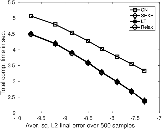
The goal of this numerical experiment is to compare the computational cost of the exponential integrator introduced in this paper to that of numerical methods from the literature. We run all numerical schemes over the time interval $[0,0.5]$ for the stochastic Manakov equation (1) with $\gamma=1$ . We discretise the spatial domain with $a=50$ , using a mesh of size $\Delta x=0.2$ . We run $500$ samples for each numerical scheme. For each scheme and each sample, we run several time steps and compare the ${\mathbb{L}}^{2}$ error at the final time with a reference solution provided for the same sample by the same scheme for a very small time step $h=2^{-16}$ . Figure 3 displays the total computational time for all the samples, for each numerical scheme and each time step, as a function of the averaged final error. One observes that the performance of the Crank–Nicolson scheme is a little bit inferior than the performance for the other numerical schemes.

4.4. Preservation of the ${\mathbb{L}}^{2}$ -norm

The next numerical experiment illustrates the preservation of the ${\mathbb{L}}^{2}$ -norm along one sample path of the above numerical schemes. For this, we consider $a=50$ , $\gamma=1$ , time interval $[0,3]$ and discretisation parameters $h=0.006$ and $\Delta x=0.25$ . The results are displayed in Figure 4. Exact preservation of the ${\mathbb{L}}^{2}$ -norm for the Crank–Nicolson, the Lie–Trotter and the relaxation schemes is observed. A small drift is observed for the exponential scheme.

4.5. ${\mathbb{L}}^{2}$ -preserving exponential integrators

As seen above, the proposed exponential integrator unfortunately does not preserve the ${\mathbb{L}}^{2}$ -norm. This can be fixed using ideas from [8, 9]. We thus propose the following modified exponential method for the numerical discretisation the stochastic Manakov equation (1)

	$\displaystyle F_{*}$	$\displaystyle=F\left(U_{h,n}X^{n}+i\frac{h}{2}F_{*}\right)$
(modEXP)		$\displaystyle X^{n+1}$	$\displaystyle=U_{h,n}X^{n}+ihF_{*},$

where we define $F(X)=|X|^{2}X$ for the nonlinearity.

As seen in the introduction, the exact solution to the stochastic Manakov equation (1) preserves the ${\mathbb{L}}^{2}$ -norm. The following proposition states that the modified exponential method enjoys the same property.

Proposition 5.

The exponential integrator (4.5) preserves the ${\mathbb{L}}^{2}$ -norm.

Proof.

By definition of the exponential integrator and using the isometry property of the discrete random propagator $U_{h,0}$ , one obtains

\left\lVert X^{1}\right\rVert^{2}=\left\lVert U_{h,0}X^{0}+ihF_{*}\right\rVert^{2}=\left\lVert X^{0}\right\rVert^{2}+h^{2}\left\lVert F_{*}\right\rVert^{2}+h(U_{h,0}X^{0},iF_{*})_{2}+h(iF_{*},U_{h,0}X^{0})_{2}.

Setting $Y:=U_{h,0}X^{0}+i\frac{h}{2}F_{*}$ or $U_{h,0}X^{0}=(Y-i\frac{h}{2}F_{*})$ , one gets

	$\displaystyle\left\lVert X^{1}\right\rVert^{2}$	$\displaystyle=\left\lVert X^{0}\right\rVert^{2}+h^{2}\left\lVert F_{}\right\rVert^{2}+h(Y-i\frac{h}{2}F_{},iF_{})_{2}+h(iF_{},Y-i\frac{h}{2}F_{*})_{2}$
		$\displaystyle=\left\lVert X^{0}\right\rVert^{2}+h^{2}\left\lVert F_{}\right\rVert^{2}+h\left((Y,iF_{})_{2}+(iF_{},Y)_{2}\right)-\frac{h^{2}}{2}\left\lVert F_{}\right\rVert-\frac{h^{2}}{2}\left\lVert F_{*}\right\rVert$
		$\displaystyle=\left\lVert X^{0}\right\rVert^{2}+2h\mathrm{Re}\left((Y,iF_{*})_{2}\right)=\left\lVert X^{0}\right\rVert^{2}+0=\left\lVert X^{0}\right\rVert^{2}$

since the ${\mathbb{L}}^{2}$ -norm is an invariant for the original problem and $F_{*}=F(Y)$ . ∎

We now numerically illustrate this property with the same parameters as in the previous numerical experiment. Figure 5 shows the exact preservation of the ${\mathbb{L}}^{2}$ -norm by the exponential scheme (4.5).

It would be of interest to prove the orders of convergence of the ${\mathbb{L}}^{2}$ -preserving exponential integrator (4.5). This is however out of the scope of this publication since it seems that one would need to use other techniques than that used in the proofs of the proposed explicit exponential integrator (3).

5. Appendix

We prove here that the operator $U_{h,n}$ defined after equation (3) is an isometry from ${\mathbb{H}}^{m}({\mathbb{R}})$ to itself for all $h>0$ and all realization of the random variable.

Proposition 6.

Let $m\in{\mathbb{N}}$ , $(u_{0},v_{0})\in{\mathbb{H}}^{m}({\mathbb{R}})$ , $h>0$ , $\chi_{1},\chi_{2},\chi_{3}\in{\mathbb{R}}$ and define a distribution $(u_{1},v_{1})\in({\mathcal{S}}^{\prime}({\mathbb{R}}))^{2}$ as the solution of

(9)

\begin{pmatrix}u_{1}\\ v_{1}\end{pmatrix}=U_{h,n}\begin{pmatrix}u_{0}\\ v_{0}\end{pmatrix}.

One has $(u_{1},v_{1})\in{\mathbb{H}}^{m}({\mathbb{R}})$ and $\left\lVert(u_{1},v_{1})\right\rVert_{{\mathbb{H}}^{m}({\mathbb{R}})}=\left\lVert(u_{0},v_{0})\right\rVert_{{\mathbb{H}}^{m}({\mathbb{R}})}$ .

Proof.

The operator $H_{h,n}$ defined after (3) acts on the Fourier transform of the couples of functions at frequency $\xi\in{\mathbb{R}}$ via the complex-valued $2\times 2$ matrix $ih\xi^{2}I_{2}+i\xi\sqrt{\gamma h}(\chi_{1}\sigma_{1}+\chi_{2}\sigma_{2}+\chi_{3}\sigma_{3})$ . This matrix reads $iS(\xi)$ where $S(\xi)$ is an hermitian $2\times 2$ matrix. Therefore, the matrix $S(\xi)$ is diagonalizable in an orthonormal basis of ${\mathbb{C}}^{2}$ with real eigenvalues $\lambda_{1}(\xi)$ and $\lambda_{2}(\xi)$ . We infer that there exists a unitary matrix $P(\xi)$ such that $S(\xi)=P(\xi)^{\star}D(\xi)P(\xi)$ , where $D(\xi)$ is the diagonal matrix with $\lambda_{1}(\xi)$ and $\lambda_{2}(\xi)$ on the diagonal. Hence, relation (9) is equivalent to

\forall\xi\in{\mathbb{R}},\hskip 18.49988ptP(\xi)\begin{pmatrix}\hat{u}_{1}(\xi)\\ \hat{v}_{1}(\xi)\end{pmatrix}=\begin{pmatrix}\frac{1-i\lambda_{1}(\xi)/2}{1+i\lambda_{1}(\xi)/2}&0\\ 0&\frac{1-i\lambda_{2}(\xi)/2}{1+i\lambda_{2}(\xi)/2}\end{pmatrix}P(\xi)\begin{pmatrix}\hat{u}_{0}(\xi)\\ \hat{v}_{0}(\xi)\end{pmatrix}.

Since the diagonal elements in the diagonal matrix above have modulus 1 and $P(\xi)$ is unitary, we infer that

\forall\xi\in{\mathbb{R}},\hskip 18.49988pt|\hat{u}_{1}(\xi)|^{2}+|\hat{v}_{1}(\xi)|^{2}=|\hat{u}_{0}(\xi)|^{2}+|\hat{v}_{0}(\xi)|^{2}.

This proves that $(u_{1},v_{1})\in{\mathbb{H}}^{m}({\mathbb{R}})$ since $(u_{0},v_{0})\in{\mathbb{H}}^{m}({\mathbb{R}})$ , and the ${\mathbb{H}}^{m}({\mathbb{R}})$ -norm of these two couples of functions is the same. ∎

References

[1] G. Agrawal. Nonlinear Fiber Optics. Electronics & Electrical. Elsevier Science, 2007.
[2] R. Anton and D. Cohen. Exponential integrators for stochastic Schrödinger equations driven by Itô noise. J. Comput. Math., 36(2):276–309, 2018.
[3] R. Anton, D. Cohen, S. Larsson, and X. Wang. Full discretization of semilinear stochastic wave equations driven by multiplicative noise. SIAM J. Numer. Anal., 54(2):1093–1119, 2016.
[4] R. Anton, D. Cohen, and L. Quer-Sardanyons. A fully discrete approximation of the one-dimensional stochastic heat equation. IMA J. Numer. Anal., 40(1):247–284, 2020.
[5] R. Belaouar, A. de Bouard, and A. Debussche. Numerical analysis of the nonlinear Schrödinger equation with white noise dispersion. Stoch. Partial Differ. Equ. Anal. Comput., 3(1):103–132, 2015.
[6] A. Berg, D. Cohen, and G. Dujardin. Lie–trotter splitting for the nonlinear stochastic Manakov system. In preparation, 2020.
[7] C. Besse, G. Dujardin, and I. Lacroix-Violet. High order exponential integrators for nonlinear Schrödinger equations with application to rotating Bose-Einstein condensates. SIAM J. Numer. Anal., 55(3):1387–1411, 2017.
[8] E. Celledoni, D. Cohen, and B. Owren. Symmetric exponential integrators with an application to the cubic Schrödinger equation. Found. Comput. Math., 8(3):303–317, 2008.
[9] D. Cohen and G. Dujardin. Exponential integrators for nonlinear Schrödinger equations with white noise dispersion. Stoch. Partial Differ. Equ. Anal. Comput., 5(4):592–613, 2017.
[10] D. Cohen and L. Gauckler. One-stage exponential integrators for nonlinear Schrödinger equations over long times. BIT, 52(4):877–903, 2012.
[11] D. Cohen, S. Larsson, and M. Sigg. A trigonometric method for the linear stochastic wave equation. SIAM J. Numer. Anal., 51(1):204–222, 2013.
[12] D. Cohen and L. Quer-Sardanyons. A fully discrete approximation of the one-dimensional stochastic wave equation. IMA J. Numer. Anal., 36(1):400–420, 2016.
[13] A. de Bouard and A. Debussche. Weak and strong order of convergence of a semidiscrete scheme for the stochastic nonlinear Schrödinger equation. Appl. Math. Optim., 54(3):369–399, 2006.
[14] A. de Bouard and M. Gazeau. A diffusion approximation theorem for a nonlinear PDE with application to random birefringent optical fibers. Ann. Appl. Probab., 22(6):2460–2504, 2012.
[15] G. Dujardin. Exponential Runge-Kutta methods for the Schrödinger equation. Appl. Numer. Math., 59(8):1839–1857, 2009.
[16] J. Garnier and R. Marty. Effective pulse dynamics in optical fibers with polarization mode dispersion. Wave Motion, 43(7):544–560, 2006.
[17] M. Gazeau. Analyse de modèles mathématiques pour la propagation de la lumière dans les fibres optiques en présence de biréfringence aléatoire. PhD thesis, Ecole Polytechnique, 2012.
[18] M. Gazeau. Numerical simulation of nonlinear pulse propagation in optical fibers with randomly varying birefringence. J. Opt. Soc. Am. B, 30(9):2443–2451, Sep 2013.
[19] M. Gazeau. Probability and pathwise order of convergence of a semidiscrete scheme for the stochastic Manakov equation. SIAM J. Numer. Anal., 52(1):533–553, 2014.
[20] A. Hasegawa. Effect of polarization mode dispersion in optical soliton transmission in fibers. Physica D: Nonlinear Phenomena, 188(3):241 – 246, 2004.
[21] M. Hochbruck and A. Ostermann. Exponential integrators. Acta Numer., 19:209–286, 2010.
[22] A. Jentzen and P. E. Kloeden. The numerical approximation of stochastic partial differential equations. Milan J. Math., 77:205–244, 2009.
[23] G. J. Lord and A. Tambue. Stochastic exponential integrators for the finite element discretization of SPDEs for multiplicative and additive noise. IMA J. Numer. Anal., 33(2):515–543, 2013.
[24] J. Printems. On the discretization in time of parabolic stochastic partial differential equations. M2AN Math. Model. Numer. Anal., 35(6):1055–1078, 2001.
[25] C.R. Wai, P.K.A.; Menyak. Polarization mode dispersion, decorrelation, and diffusion in optical fibers with randomly varying birefringence. Journal of Lightwave Technology, 14, 1996.
[26] X. Wang. An exponential integrator scheme for time discretization of nonlinear stochastic wave equation. J. Sci. Comput., 64(1):234–263, 2015.

Exponential integrators for the stochastic Manakov equation

Abstract.

1. Introduction

2. Setting and notation

Theorem 1 (Theorem 1.2 in [14]).

3. Convergence analysis of the exponential integrator

3.1. The Lipschitz-continuous case

Theorem 2.

Proof.

3.2. Convergence in the non-Lipschitz case

Proposition 3.

Proof.

Proposition 4.

Proof.

4. Numerical experiments

4.1. Evolution plots

4.2. Strong convergence

4.3. Computational costs

4.4. Preservation of the 𝕃2{\mathbb{L}}^{2}-norm

4.5. 𝕃2{\mathbb{L}}^{2}-preserving exponential integrators

Proposition 5.

Proof.

5. Appendix

Proposition 6.

Proof.

References

4.4. Preservation of the ${\mathbb{L}}^{2}$ -norm

4.5. ${\mathbb{L}}^{2}$ -preserving exponential integrators