Mean-field study of the Bose-Hubbard model in Penrose lattice

Quasicrystals have aperiodic structure different from fully disordered one. Although translational symmetry is absent, the presence of sharp spots in Bragg reflection indicates long-range order Shechtman et al. 1984; Levine and Steinhardt 1984. Quasicrystals can be realized even in bilayer graphene Yao et al. 2018 and photonic lattices Jin and Gao 2012. In addition to various characteristics due to aperiodicity Steurer 2018; Louzguine-Luzgin and Inoue 2008, recent new findings expand the field of quasicrystal to include superconductivity Kamiya et al. 2018; Araújo and Andrade 2019; Sakai et al. 2017; Sakai and Arita 2019, quantum criticality Deguchi et al. 2012; Otsuki and Kusunose 2016, and topology Lang et al. 2012; Matsuda et al. 2014; Dareau et al. 2017; Spurrier and Cooper 2019; Huang and Liu 2018. In general, self-similarity in quasicrystals dictates fractal structure in wavefunction and phase diagram  Ghadimi et al. 2017; Bandres et al. 2016. This characteristic is justified by the presence of the inflation and deflation rules to construct quasicrystals Ma and Liu 1989.

One of the well-known two-dimensional (2D) quasicrystals is the so-called Penrose lattice de Bruijn 1981a; de Bruijn 1981b. One can construct the lattice using inflation, projection, or multi-grade rules. The Penrose lattice has been studied intensively Oitmaa et al. 1990; Liu and Ma 1991; Szallas and Jagannathan 2008; Vignolo et al. 2016; Takemori and Koga 2015; Koga and Tsunetsugu 2017; Takemori et al. 2018; Jagannathan 2012; Szallas et al. 2009; Murakami et al. 2020 and its structure dictates thermodynamically degenerate states in energy spectrum Arai et al. 1988; Fujiwara et al. 1988.

Ultracold gases in optical lattices provide us an ideal playground of strong correlation Bloch 2005 and also quasicrystals Singh et al. 2015; Guidoni et al. 1997; Sanchez-Palencia and Santos 2005; Corcovilos and Mittal 2019; Hou et al. 2018; Gopalakrishnan et al. 2013, which allows us to investigate the interplay of strong correlation and aperiodicity. A typical strongly correlated system in optical lattice is the Bose-Hubbard model, where phase transition between Mott insulator (MI) to superfluid (SF) phase appears Fisher et al. 1989; Dutta et al. 2015 as experimentally observed Jaksch et al. 1998; Greiner et al. 2002. The Bose-Hubbard model is also used to describe the effective low-energy theory of superconducting films and arrays of Josephson junctions Giamarchi et al. 2008; Nikuni et al. 2000; Bruder et al. 1993. Recent achievements in establishing an eight-fold rotationally symmetric optical lattice attract new attention Viebahn et al. 2019, in connection with theoretical investigation of an extended Bose-Hubbard with quasicrystalline confined potential Johnstone et al. 2019, where spontaneous breaking of underlying eight-fold symmetry is observed. However, the effect of aperiodicity in the Bose-Hubbard model is not yet fully understood both theoretically and experimentally.

In this paper, we investigate the phase diagram of the Bose-Hubbard model in the Penrose lattice. We use a self-consistent mean-field theory and find that the distribution of Bose condensate in the Penrose lattice exhibits a fractal structure near the MI-SF boundary. We attribute the appearance of the fractal structure to a consequence of the divergence of correlation length seen in any phase transition. Therefore, the fractal structure is a common signature of phase transition in quasiperiodic systems.

The arrangement of this paper is as follows. In Sec. II, we describe our Bose-Hubbard model on the Penrose lattice and mean-field treatment. The classification of lattice sites (vertices) is also introduced. In Sec. III, we discuss the result of phase diagram, local superfluid amplitude, and a critical behavior of several quantities. A fractal structure near the phase transition in the perpendicular space in the Penrose lattice is also discussed. Finally, a summary is given in Sec. IV.

The Hamiltonian of the single-band Bose-Hubbard model is defined by

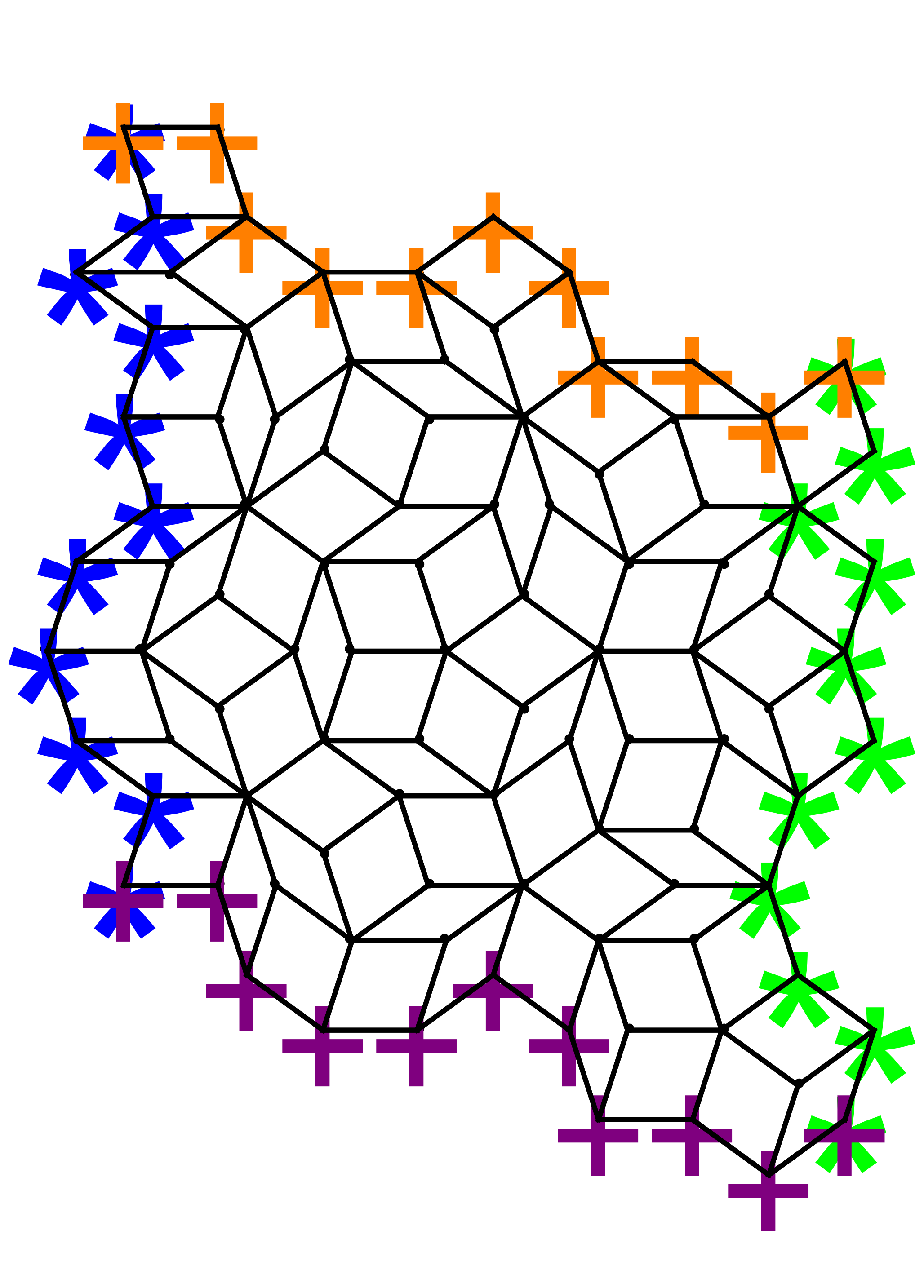
where $\hat{b}_{i}$ and $\hat{b}^{\dagger}_{i}$ are annihilation and creation operators of bosons at site $i$ and the number operator $\hat{n}_{i}=\hat{b}^{\dagger}_{i}\hat{b}_{i}$. We refer the site to vertex, which is denoted by circles in Fig. 1(a). The summation $\langle i,j\rangle$ represents nearest-neighbor (NN) links in the Penrose lattice shown as short bar connecting two vertices in Fig. 1(a). $J$, $\mu$, and $U$ in Eq. (1) are the hopping energy of boson, the chemical potential, and on-site Coulomb interaction, respectively. We note that hopping processes with the shortest inter-vertex distance, for example, hopping between numbers 8 and 9 in Fig. 1(a), are not included in Eq.(1). This exclusion guarantees bipartite properties of this Penrose lattice.

Because of the presence of the hopping term in Eq. (1), the exact solution is inaccessible. Therefore, we use a mean-field technique and decouple the hopping term using local superfluid amplitude $\langle\hat{b}_{i}\rangle$. The resulting mean-field Hamiltonian is given by $H_{\mathrm{MF}}=\sum_{i}H_{i}+E_{0}$ with

where $\psi_{i}=\sum_{j\in\text{NN.i}}\langle\hat{b}_{j}\rangle$ with summation over NN links connected to the vertex $i$ and $E_{0}=J\sum\psi^{*}_{i}\langle\hat{b}_{i}\rangle$.

In order to obtain a self-consistent solution of Eq. (2) in the local Hilbert space containing maximally $n_{\mathrm{b}}$ bosons, we start with an initial $\psi_{i}$ and then calculate $\langle\hat{n}_{i}\rangle$ and $\langle\hat{b}_{i}\rangle$ using the ground-state wavefunction for each vertex. We continue updating $\psi_{i}$ until the convergence of $\langle\hat{n}_{i}\rangle$ and $\langle\hat{b}_{i}\rangle$ is obtained within a certain tolerance ($10^{-9}$ in our case). This self-consistent procedure gives rise to site-dependent distribution of $\langle\hat{n}_{i}\rangle$ and $\langle\hat{b}_{i}\rangle$ on the Penrose lattice. This technique is sometimes called inhomogeneous mean-field theory Pai et al. 2012; Kurdestany et al. 2012, which gives equivalent results with variational Gutzwiiler method Pisarski et al. 2011; McIntosh et al. 2012; Barman and Basu 2014; Yi et al. 2007; Sheshadri et al. 1995; Niederle and Rieger 2015; Rokhsar and Kotliar 1991; Krauth et al. 1992. We note that this self-consistent procedure gives moderately consistent results compared by quantum Monte Carlo simulations in determining the phase diagram of the Bose-Hubbard model with NN repulsion interaction Ohgoe et al. 2012.

We take $n_{\mathrm{b}}=7$. Within our mean-field theory, we generally find the MI and SF phases in the Bose-Hubbard model. In the MI phase, all sites have equal integer number of bosons and thus $\langle\hat{b}_{i}\rangle=0$. On the other hand, $\langle\hat{b}_{i}\rangle$ is nonzero for the SF phase. In our method, we find order parameters on all vertices. Therefore, we can check the existence of exotic states like Bose-glass, supersolid, and density-wave phases. We did not see these phases in our model. This is reasonable since these phases appear in the presence of disorder and/or NN interaction in Eq. (1) Iskin 2011; Kurdestany et al. 2012; Sheshadri et al. 1995. To minimize the boundary effects, we apply periodic boundary conditions (PBC) in an approximant of Penrose lattice containing $N=167761$ vertices (For detail, see the Appendix. A) Entin-Wohlman et al. 1988; Babalievski and Peshev 1990; Tsunetsugu et al. 1991.

In the Penrose lattice, we can classify vertices in terms of their local environment. For this classification, we first find the number of NN links, $M_{1}$, i.e., the total number of paths using one link ($M_{k}$ with $k=1$ and see the second row in Table 1), which is equivalent to coordination number for each vertex in Fig. 1(a). $M_{1}$ changes from $3$ to $7$. This means that all of sites are indexed by five kinds of vertices. Next, we count the number of NN vertices having $l$ links, $m_{1}^{(l)}$, and make a list of them (the third-seventh rows in Table 1). From the list of $m_{1}^{(l)}$ together with $M_{1}$, we find fourteen types of configurations, meaning that all of sites are indexed by fourteen kinds of vertices. The total number of paths using two links ($k=2$) from a given vertex is then expressed as $M_{2}=\sum_{l=3}^{7}m_{1}^{(l)}l$, which is listed in the eighth row of Table 1. We repeat this listing for the vertices accessed by using the two links form a given vertex, which is shown in the ninth-thirteenth rows as $m_{2}^{(l)}$. In the last row of Table 1, the total number of paths using three links ($k=3$) from a given vertex ($M_{3}=\sum_{l=3}^{7}m_{2}^{(l)}l$) is listed. Performing this procedure for all vertices in our supercell, we find that there are twenty-seven kinds of vertices, by which almost the whole system is covered. They are indexed as $\alpha(=1,2,\cdots,27)$ in the first row of Table 1. We note that, in our approximant periodic lattice with $N=167761$ vertices, there are vertices that do not belong to the 27 types around defects, but we can ignore them since the total number of the defects is just 2.

We call the number of distinct vertices for a given $k$ the number of classes (NoC). For example, NoC is equal to 5, 14, and 27 for $k=1$, 2, and 3, respectively. We draw a small portion of Penrose lattice in Fig. 1(a), where each vertex has an index $\alpha(=1,2,\cdots,27)$ and color indicating its class obtained for $k=3$. We can increase $k$ as many as possible. We find NoC $\propto k^{1.84}$ in the large $k$ region (see Fig. 3(c)). We will come back to this point later.

As explained in the Appendix. A, vertexes in the Penrose lattice can be labeled with five integers, originated from cut and projection of five dimensional cubic lattice Koga and Tsunetsugu 2017. One can construct original Penrose lattice by mapping those labels. However, using another mapping, one finds four different 2D structures, called perpendicular space, where we assign the four structures to $\mathcal{Z}=1$, 2, 3, and 4 [see Figs. 1(b) and 1(c) for $\mathcal{Z}=1$ and 2, respectively]. We can divide perpendicular space into symmetric sections, where each section represents vertex with similar local circumstances. Therefore, one notices the index $\alpha$ in Fig. 1(a) mapped to different sections in the perpendicular space [see Figs. 1(b) and 1(c)]. We note that the bipartite property of Penrose lattice leads to the fact that $\mathcal{Z}=1,3$ and $\mathcal{Z}=2,4$ belong to different subsystems, though the same $\alpha$ are shared among them.

We first examine the phase diagram of the Bose-Hubbard model on the Penrose lattice. From the calculation of two order parameters per vertex, $\langle\hat{n}_{i}\rangle$ and $\langle\hat{b}_{i}\rangle$, for the Bose-Hubbard model without disorder and/or inter-site interaction, we expect two phases: one is MI with $\langle\hat{b}_{i}\rangle=0$ and $\langle\hat{n}_{i}\rangle=n_{0}$ ($n_{0}=1,2,\cdots$, corresponding to bosonic occupation number at each vertex), and the other is SF with $\langle\hat{b}_{i}\rangle\neq 0$. In fact, we find none of Bose-glass, density wave, and supersolid phases in the phase diagram. Figure 2 shows the phase diagram, where we find MI phases denoted by MI$n_{0}$ and SF. Since averaged coordination number in the Penrose lattice is $\bar{z}=4$, which is the same as the coordination number $z=4$ in the square lattice, the phase boundary between MI and SF is expected to be similar to that of the square lattice. This is the case as shown by the dashed orange curve along MI lobes in Fig. 2, which is mean-field phase boundary for the square lattice given analytically van Oosten et al. 2001; Freericks and Monien 1994 by

where $s=\text{round}(\mu/U+1/2)$. The similarity indicates small effect of aperiodicity on the phase boundary.

In the SF phase of square lattice, the local superfluid amplitude $\langle\hat{b}_{i}\rangle$ is uniform, i.e., independent of $i$, for any region in the phase diagram. On the other hand, nonuniform distribution of $\langle\hat{b}_{i}\rangle$ in the Penrose lattice is easily expected from the presence of different types of vertices as shown in Fig. 1(a). Then, an arising question is how its nonuniform distribution changes in the phase diagram. To see this, we define an $\alpha$ dependent average of $\langle\hat{b}_{i}\rangle$ as $\overline{b}_{\alpha}=N_{\alpha}^{-1}\sum_{i\in\alpha}\langle\hat{b}_{i}\rangle$, where $N_{\alpha}$ is the number of $\alpha$-type vertex in the whole lattice. This quantity can distinguish the twenty-seven classes of vertices. However, each class should have further internal structure coming from possible extension of NoC for $k\geq 4$. To recognize this structure, we also define a mean deviation of local superfluid amplitude distribution as $\delta b_{\alpha}=\sqrt{N_{\alpha}^{-1}\sum_{i\in\alpha}(\langle\hat{b}_{i}\rangle-\overline{b}_{\alpha})^{2}}$.

With approaching phase transition from the superfluid side, the average value of local superfluid amplitude, $\overline{b}=\sum_{i}\langle\hat{b}_{i}\rangle/N$ with $N=\sum_{\alpha}N_{\alpha}$, reduces its value toward zero as shown in the inset of Fig. 3(a). At the same time, both $\overline{b}_{\alpha}$ and $\delta\overline{b}_{\alpha}$ become smaller. Therefore, we use $\delta\overline{b}_{\alpha}/\overline{b}$ to evaluate the magnitude of the mean deviation of $\delta\overline{b}_{\alpha}$. Note that the larger $\delta b_{\alpha}/\overline{b}$ is, the deeper the internal structure is.

In Fig. 3(a), we plot $\overline{b}_{\alpha}/\overline{b}$ and $\delta b_{\alpha}/\overline{b}$ as a function of $\bar{z}J/U$ along the horizontal dotted line ($\mu/U=0.8$) in Fig. 2. We note that $\delta b_{\alpha}/\overline{b}$ is denoted by the length of bars for each $\overline{b}_{\alpha}/\overline{b}$. At large $\bar{z}J/U$ far from the phase boundary, $\overline{b}_{\alpha}/\overline{b}$ is tend to be grouped accompanied by negligibly small $\delta b_{\alpha}/\overline{b}$. In the limit of $\bar{z}J/U\rightarrow\infty$, $\overline{b}_{\alpha}/\overline{b}$ is grouped into five classes equivalent to the coordination number, i.e., NoC for $k=1$. This means that, if correlation effect is small, the coordination number controls physical properties as expected. On the other hand, with approaching $\bar{z}J/U$ to the phase boundary, the mean deviation $\delta b_{\alpha}/\overline{b}$ becomes large. This means that the number of distinct vertices with different local superfluid amplitude increases with approaching to the boundary. In other words, long-distant correlation becomes important in order to obtain critical behaviors near the phase transition.

In order to make critical behaviors visible, we introduce a new quantity that can characterize distinct number of vertices more than twenty seven. We use $\langle\hat{b}_{i}\rangle$ itself for this purpose, and try to find how many distinct values exist with approaching to the phase boundary. For distinguishing different value of local superfluid amplitude, we i) make shifting and scaling for $\langle\hat{b}_{i}\rangle$ to be located within $[0,1]$. This is done by evaluating $\left(\langle\hat{b}_{i}\rangle-\text{min}[{\{\langle\hat{b}_{i}\rangle\}}]\right)/\left(\text{max}[{\{\langle\hat{b}_{i}\rangle\}}]-\text{min}[{\{\langle\hat{b}_{i}\rangle\}}]\right)$, where min and max denote minimum and maximum among all values of local superfluid amplitude, respectively. Then, we ii) sort the scaled $\langle\hat{b}_{i}\rangle$ from 0 to 1, iii) calculate the difference of $\langle\hat{b}_{i}\rangle$ between $i$ and $i+1$ from $i=1$ to $i=N-1$, and iv) count the number of the difference (gap) whose magnitude is more than a given small threshold value. We call this number the number of gap (NoG). For example, NoG is zero for the square lattice because $\langle\hat{b}_{i}\rangle$ is independent of $i$. In the Penrose lattice, we have NoG$=4$ in the large limit of $\bar{z}J/U$ since there are five distinct values of $\langle\hat{b}_{i}\rangle$. We show log-log plot of NoG in Fig. 3(b) along the horizontal dotted line in Fig. 2, where four different threshold values, $10^{-5}$ , $5\times 10^{-6}$, $10^{-6}$, and $5\times 10^{-7}$ are used. With approaching to the phase boundary at $\bar{z}J_{c}/U\approx 0.0835$, NoG increases, indicating the increase of distinct vertices with different local superfluid amplitude. Interesting is that, with decreasing the threshold value, NoG rapidly increases near the boundary and shows a diverging behavior with an approximate exponent around $-0.9$, i.e., NoG $\propto(J-J_{c})^{-0.9}$. This resembles to a critical behavior toward continuous phase transition as suggested from the vanishing of averaged order parameter $\bar{b}$ [see inset of Fig 3(a)].

In order to understand this diverging behavior more, we focus on the fact that the increase of NoG corresponds to the increase of distinct vertices with different local superfluid amplitude. The latter is measured by NoC, whose large region is proportional to $k^{1.84}$ as shown in Fig. 3(c). Therefore, diverging behavior in NoG is directly connected to diverging behavior in NoC at large $k$. Since $k$ represents the number of links from a given vertex, we may regard $k$ as a measure of correlation length $\xi$ from a given vertex. Based on this reasoning, we have NoG $\propto$ NoC $\propto k^{1.84}\propto\xi^{1.84}$. Since $\xi\propto(J-J_{c})^{-0.5}$ for the mean-field phase transition, we finally expect that NoG $\propto(J-J_{c})^{-0.92}$, whose exponent is close to the calculated one in NoG, $\approx-0.9$. This indicates that diverging behavior in NoG is a consequence of criticality in the mean-field phase transition. We note that this critical behavior does not appear if $\mu/U=n_{0}$ and $J/U\rightarrow 0$. We suggest that the assumption of $\xi\propto k$ may change if we alter the class of universality. We leave this to future work.

Usefulness of perpendicular space presentation has already been found in considering magnetism on the Penrose lattice Koga and Tsunetsugu 2017; Szallas and Jagannathan 2008. Therefore, we show the perpendicular space representation of $\langle\hat{b}_{i}\rangle$ in Fig. 4 for two sets of parameters at the end of the red dashed line in Fig. 2. We recognize notable differences in the two cases. For the parameter far from the phase boundary, we find fourteen distinct sections in Figs. 4(c) and 4(d). The number corresponds to the number of distinct vertices obtained by setting $k=2$ as discussed above. On the other hand, for the parameter close to the phase boundary, we can see a fractal structure in Figs. 4(a) and 4(b). For example, we find a various size of star structure inside stars. We can understand the emergence of the fractal structure near the phase transition as follows. Because of diverging behavior in NoG near the MI-SF phase boundary, all distances become relevant. We have found from the previous discussion that tracing far distant links by increasing $k$ enhances NoC dramatically. Therefore we can expect further distinguishable sections in the perpendicular space, resulting in fractal nature. In other words, a combination of criticality leading to phase transition and aperiodicity is a key for the emergence of fractal structure.

We have obtained mean-field phase diagram in the Penrose-Bose-Hubbard model. We have found that the Penrose lattice does not change the MI-SF boundary drastically in comparison with square lattice. However, the spatial distribution of Bose condensate is unequal, and indeed fractal structure appears in the perpendicular representation of local superfluid amplitude near the MI-SF phase transition. This is a consequence of the cooperative effect of criticality leading to phase transition and quasiperiodicity, which is expected to be a common feature in aperiodic strongly correlated systems.

This work was supported by Challenging Research Exploratory (Grant No. JP17K18764), Grant-in-Aid for Scientific Research on Innovative Areas (Grant No. JP19H05821).

References

- Shechtman et al. (1984) D. Shechtman, I. Blech, D. Gratias, and J. W. Cahn, “Metallic phase with long-range orientational order and no translational symmetry,” Phys. Rev. Lett. 53, 1951–1953 (1984).
- Levine and Steinhardt (1984) Dov Levine and Paul Joseph Steinhardt, “Quasicrystals: A new class of ordered structures,” Phys. Rev. Lett. 53, 2477–2480 (1984).
- Yao et al. (2018) Wei Yao, Eryin Wang, Changhua Bao, Yiou Zhang, Kenan Zhang, Kejie Bao, Chun Kai Chan, Chaoyu Chen, Jose Avila, Maria C. Asensio, Junyi Zhu, and Shuyun Zhou, “Quasicrystalline 30 twisted bilayer graphene as an incommensurate superlattice with strong interlayer coupling,” Proceedings of the National Academy of Sciences 115, 6928–6933 (2018).
- Jin and Gao (2012) Wentao Jin and Yuanmei Gao, “Optically induced two-dimensional photonic quasicrystal lattices in iron-doped lithium niobate crystal with an amplitude mask,” Applied Physics Letters 101, 141104 (2012).
- Steurer (2018) Walter Steurer, “Quasicrystals: What do we know? What do we want to know? What can we know?” Acta Crystallographica Section A 74, 1–11 (2018).
- Louzguine-Luzgin and Inoue (2008) D.V. Louzguine-Luzgin and A. Inoue, “Formation and properties of quasicrystals,” Annual Review of Materials Research 38, 403–423 (2008).
- Kamiya et al. (2018) K. Kamiya, T. Takeuchi, N. Kabeya, N. Wada, T. Ishimasa, A. Ochiai, K. Deguchi, K. Imura, and N. K. Sato, “Discovery of superconductivity in quasicrystal,” Nature Communications 9, 154 (2018).
- Araújo and Andrade (2019) Ronaldo N. Araújo and Eric C. Andrade, “Conventional superconductivity in quasicrystals,” Phys. Rev. B 100, 014510 (2019).
- Sakai et al. (2017) Shiro Sakai, Nayuta Takemori, Akihisa Koga, and Ryotaro Arita, “Superconductivity on a quasiperiodic lattice: Extended-to-localized crossover of cooper pairs,” Phys. Rev. B 95, 024509 (2017).
- Sakai and Arita (2019) Shiro Sakai and Ryotaro Arita, “Exotic pairing state in quasicrystalline superconductors under a magnetic field,” Phys. Rev. Research 1, 022002 (2019).
- Deguchi et al. (2012) Kazuhiko Deguchi, Shuya Matsukawa, Noriaki K. Sato, Taisuke Hattori, Kenji Ishida, Hiroyuki Takakura, and Tsutomu Ishimasa, “Quantum critical state in a magnetic quasicrystal,” Nature Materials 11, 1013–1016 (2012).
- Otsuki and Kusunose (2016) Junya Otsuki and Hiroaki Kusunose, “Distributed hybridization model for quantum critical behavior in magnetic quasicrystals,” Journal of the Physical Society of Japan 85, 073712 (2016).
- Lang et al. (2012) Li-Jun Lang, Xiaoming Cai, and Shu Chen, “Edge states and topological phases in one-dimensional optical superlattices,” Phys. Rev. Lett. 108, 220401 (2012).
- Matsuda et al. (2014) Fuyuki Matsuda, Masaki Tezuka, and Norio Kawakami, “Topological properties of ultracold bosons in one-dimensional quasiperiodic optical lattice,” Journal of the Physical Society of Japan 83, 083707 (2014).
- Dareau et al. (2017) A. Dareau, E. Levy, M. Bosch Aguilera, R. Bouganne, E. Akkermans, F. Gerbier, and J. Beugnon, “Revealing the topology of quasicrystals with a diffraction experiment,” Phys. Rev. Lett. 119, 215304 (2017).
- Spurrier and Cooper (2019) Stephen Spurrier and Nigel R. Cooper, “Theory of quantum oscillations in quasicrystals: Quantizing spiral fermi surfaces,” Phys. Rev. B 100, 081405 (2019).
- Huang and Liu (2018) Huaqing Huang and Feng Liu, “Quantum spin hall effect and spin bott index in a quasicrystal lattice,” Phys. Rev. Lett. 121, 126401 (2018).
- Ghadimi et al. (2017) Rasoul Ghadimi, Takanori Sugimoto, and Takami Tohyama, “Majorana zero-energy mode and fractal structure in fibonacci–kitaev chain,” Journal of the Physical Society of Japan 86, 114707 (2017).
- Bandres et al. (2016) Miguel A. Bandres, Mikael C. Rechtsman, and Mordechai Segev, “Topological photonic quasicrystals: Fractal topological spectrum and protected transport,” Phys. Rev. X 6, 011016 (2016).
- Ma and Liu (1989) Penghui Ma and Youyan Liu, “Inflation rules, band structure, and localization of electronic states in a two-dimensional penrose lattice,” Phys. Rev. B 39, 9904–9911 (1989).
- de Bruijn (1981a) N.G. de Bruijn, “Algebraic theory of penrose’s non-periodic tilings of the plane. i,” Indagationes Mathematicae (Proceedings) 84, 39 – 52 (1981a).
- de Bruijn (1981b) N.G. de Bruijn, “Algebraic theory of penrose’s non-periodic tilings of the plane. ii,” Indagationes Mathematicae (Proceedings) 84, 53 – 66 (1981b).
- Oitmaa et al. (1990) J Oitmaa, M Aydin, and M J Johnson, “Antiferromagnetic ising model on the penrose lattice,” Journal of Physics A: Mathematical and General 23, 4537 (1990).
- Liu and Ma (1991) Youyan Liu and Penghui Ma, “Electronic properties of two-dimensional quasicrystals with near-neighbor interactions,” Phys. Rev. B 43, 1378–1384 (1991).
- Szallas and Jagannathan (2008) Attila Szallas and Anuradha Jagannathan, “Spin waves and local magnetizations on the penrose tiling,” Phys. Rev. B 77, 104427 (2008).
- Vignolo et al. (2016) Patrizia Vignolo, Matthieu Bellec, Julian Böhm, Abdoulaye Camara, Jean-Marc Gambaudo, Ulrich Kuhl, and Fabrice Mortessagne, “Energy landscape in a penrose tiling,” Phys. Rev. B 93, 075141 (2016).
- Takemori and Koga (2015) Nayuta Takemori and Akihisa Koga, “DMFT study of the local correlation effects in quasi-periodic system,” Journal of Physics: Conference Series 592, 012038 (2015).
- Koga and Tsunetsugu (2017) Akihisa Koga and Hirokazu Tsunetsugu, “Antiferromagnetic order in the hubbard model on the penrose lattice,” Phys. Rev. B 96, 214402 (2017).
- Takemori et al. (2018) Nayuta Takemori, Akihisa Koga, and Hartmut Hafermann, “Intersite electron correlations on inhomogeneous lattices: a real-space dual fermion approach,” (2018), arXiv:1801.02441 [cond-mat.str-el] .
- Jagannathan (2012) A. Jagannathan, “Quasiperiodic heisenberg antiferromagnets in two dimensions,” The European Physical Journal B 85, 68 (2012).
- Szallas et al. (2009) Attila Szallas, Anuradha Jagannathan, and Stefan Wessel, “Phason-disordered two-dimensional quantum antiferromagnets,” Phys. Rev. B 79, 172406 (2009).
- Murakami et al. (2020) Yuta Murakami, Denis Golež, Tatsuya Kaneko, Akihisa Koga, Andrew J. Millis, and Philipp Werner, “Collective modes in excitonic insulators: Effects of electron-phonon coupling and signatures in the optical response,” Phys. Rev. B 101, 195118 (2020).
- Arai et al. (1988) Masao Arai, Tetsuji Tokihiro, Takeo Fujiwara, and Mahito Kohmoto, “Strictly localized states on a two-dimensional penrose lattice,” Phys. Rev. B 38, 1621–1626 (1988).
- Fujiwara et al. (1988) Takeo Fujiwara, Masao Arai, Tetsuji Tokihiro, and Mahito Kohmoto, “Localized states and self-similar states of electrons on a two-dimensional penrose lattice,” Phys. Rev. B 37, 2797–2804 (1988).
- Bloch (2005) Immanuel Bloch, “Ultracold quantum gases in optical lattices,” Nature Physics 1, 23–30 (2005).
- Singh et al. (2015) K. Singh, K. Saha, S. A. Parameswaran, and D. M. Weld, “Fibonacci optical lattices for tunable quantum quasicrystals,” Phys. Rev. A 92, 063426 (2015).
- Guidoni et al. (1997) L. Guidoni, C. Triché, P. Verkerk, and G. Grynberg, “Quasiperiodic optical lattices,” Phys. Rev. Lett. 79, 3363–3366 (1997).
- Sanchez-Palencia and Santos (2005) L. Sanchez-Palencia and L. Santos, “Bose-einstein condensates in optical quasicrystal lattices,” Phys. Rev. A 72, 053607 (2005).
- Corcovilos and Mittal (2019) Theodore A. Corcovilos and Jahnavee Mittal, “Two-dimensional optical quasicrystal potentials for ultracold atom experiments,” Appl. Opt. 58, 2256–2263 (2019).
- Hou et al. (2018) Junpeng Hou, Haiping Hu, Kuei Sun, and Chuanwei Zhang, “Superfluid-quasicrystal in a bose-einstein condensate,” Phys. Rev. Lett. 120, 060407 (2018).
- Gopalakrishnan et al. (2013) Sarang Gopalakrishnan, Ivar Martin, and Eugene A. Demler, “Quantum quasicrystals of spin-orbit-coupled dipolar bosons,” Phys. Rev. Lett. 111, 185304 (2013).
- Fisher et al. (1989) Matthew P. A. Fisher, Peter B. Weichman, G. Grinstein, and Daniel S. Fisher, “Boson localization and the superfluid-insulator transition,” Phys. Rev. B 40, 546–570 (1989).
- Dutta et al. (2015) Omjyoti Dutta, Mariusz Gajda, Philipp Hauke, Maciej Lewenstein, Dirk-Sören Lühmann, Boris A Malomed, Tomasz Sowiński, and Jakub Zakrzewski, “Non-standard hubbard models in optical lattices: a review,” Reports on Progress in Physics 78, 066001 (2015).
- Jaksch et al. (1998) D. Jaksch, C. Bruder, J. I. Cirac, C. W. Gardiner, and P. Zoller, “Cold bosonic atoms in optical lattices,” Phys. Rev. Lett. 81, 3108–3111 (1998).
- Greiner et al. (2002) Markus Greiner, Olaf Mandel, Tilman Esslinger, Theodor W. Hänsch, and Immanuel Bloch, “Quantum phase transition from a superfluid to a mott insulator in a gas of ultracold atoms,” Nature 415, 39–44 (2002).
- Giamarchi et al. (2008) Thierry Giamarchi, Christian Rüegg, and Oleg Tchernyshyov, “Bose–einstein condensation in magnetic insulators,” Nature Physics 4, 198–204 (2008).
- Nikuni et al. (2000) T. Nikuni, M. Oshikawa, A. Oosawa, and H. Tanaka, “Bose-einstein condensation of dilute magnons in ,” Phys. Rev. Lett. 84, 5868–5871 (2000).
- Bruder et al. (1993) C. Bruder, Rosario Fazio, and Gerd Schön, “Superconductor–mott-insulator transition in bose systems with finite-range interactions,” Phys. Rev. B 47, 342–347 (1993).
- Viebahn et al. (2019) Konrad Viebahn, Matteo Sbroscia, Edward Carter, Jr-Chiun Yu, and Ulrich Schneider, “Matter-wave diffraction from a quasicrystalline optical lattice,” Phys. Rev. Lett. 122, 110404 (2019).
- Johnstone et al. (2019) Dean Johnstone, Patrik Öhberg, and Callum W. Duncan, “Mean-field phases of an ultracold gas in a quasicrystalline potential,” Phys. Rev. A 100, 053609 (2019).
- Pai et al. (2012) Ramesh V. Pai, Jamshid Moradi Kurdestany, K. Sheshadri, and Rahul Pandit, “Bose-hubbard models in confining potentials: Inhomogeneous mean-field theory,” Phys. Rev. B 85, 214524 (2012).
- Kurdestany et al. (2012) J.M. Kurdestany, R.V. Pai, and R. Pandit, “The inhomogeneous extended bose-hubbard model: A mean-field theory,” Annalen der Physik 524, 234–244 (2012), https://onlinelibrary.wiley.com/doi/pdf/10.1002/andp.201100274 .
- Pisarski et al. (2011) P. Pisarski, R. M. Jones, and R. J. Gooding, “Application of a multisite mean-field theory to the disordered bose-hubbard model,” Phys. Rev. A 83, 053608 (2011).
- McIntosh et al. (2012) T. McIntosh, P. Pisarski, R. J. Gooding, and E. Zaremba, “Multisite mean-field theory for cold bosonic atoms in optical lattices,” Phys. Rev. A 86, 013623 (2012).
- Barman and Basu (2014) Apurba Barman and Saurabh Basu, “Phase diagram of trapped bosons in a kagome lattice—application of inhomogeneous mean field theory,” Journal of Physics B: Atomic, Molecular and Optical Physics 47, 025302 (2014).
- Yi et al. (2007) S. Yi, T. Li, and C. P. Sun, “Novel quantum phases of dipolar bose gases in optical lattices,” Phys. Rev. Lett. 98, 260405 (2007).
- Sheshadri et al. (1995) K. Sheshadri, H. R. Krishnamurthy, Rahul Pandit, and T. V. Ramakrishnan, “Percolation-enhanced localization in the disordered bosonic hubbard model,” Phys. Rev. Lett. 75, 4075–4078 (1995).
- Niederle and Rieger (2015) A. E. Niederle and H. Rieger, “Bosons in a two-dimensional bichromatic quasiperiodic potential: Analysis of the disorder in the bose-hubbard parameters and phase diagrams,” Phys. Rev. A 91, 043632 (2015).
- Rokhsar and Kotliar (1991) Daniel S. Rokhsar and B. G. Kotliar, “Gutzwiller projection for bosons,” Phys. Rev. B 44, 10328–10332 (1991).
- Krauth et al. (1992) Werner Krauth, Michel Caffarel, and Jean-Philippe Bouchaud, “Gutzwiller wave function for a model of strongly interacting bosons,” Phys. Rev. B 45, 3137–3140 (1992).
- Ohgoe et al. (2012) Takahiro Ohgoe, Takafumi Suzuki, and Naoki Kawashima, “Ground-state phase diagram of the two-dimensional extended bose-hubbard model,” Phys. Rev. B 86, 054520 (2012).
- Iskin (2011) M. Iskin, “Route to supersolidity for the extended bose-hubbard model,” Phys. Rev. A 83, 051606 (2011).
- Entin-Wohlman et al. (1988) O Entin-Wohlman, M Kléman, and A Pavlovitch, “Penrose tiling approximants,” Journal de Physique 49, 587–598 (1988).
- Babalievski and Peshev (1990) F. Babalievski and O. Peshev, “An algorithm to construct quasilattices and study percolation on them,” Computer Physics Communications 60, 27 – 30 (1990).
- Tsunetsugu et al. (1991) Hirokazu Tsunetsugu, Takeo Fujiwara, Kazuo Ueda, and Tetsuji Tokihiro, “Electronic properties of the penrose lattice. i. energy spectrum and wave functions,” Phys. Rev. B 43, 8879–8891 (1991).
- van Oosten et al. (2001) D. van Oosten, P. van der Straten, and H. T. C. Stoof, “Quantum phases in an optical lattice,” Phys. Rev. A 63, 053601 (2001).
- Freericks and Monien (1994) J. K Freericks and H Monien, “Phase diagram of the bose-hubbard model,” Europhysics Letters (EPL) 26, 545–550 (1994).
- Senechal (1996) Marjorie Senechal, Quasicrystals and geometry (cambridge university press, 1996).
- Babalievski (1993) F.V Babalievski, “Percolation conductivity of penrose lattices by the transfer-matrix monte carlo method,” Journal of Non-Crystalline Solids 153-154, 370 – 374 (1993), proceddings of the Fourth International Conference on Quasicrystals.