Spanning attack: reinforce black-box attacks
with unlabeled data
Abstract
Adversarial black-box attacks aim to craft adversarial perturbations by querying input–output pairs of machine learning models. They are widely used to evaluate the robustness of pre-trained models. However, black-box attacks often suffer from the issue of query inefficiency due to the high dimensionality of the input space, and therefore incur a false sense of model robustness. In this paper, we relax the conditions of the black-box threat model, and propose a novel technique called the spanning attack. By constraining adversarial perturbations in a low-dimensional subspace via spanning an auxiliary unlabeled dataset, the spanning attack significantly improves the query efficiency of a wide variety of existing black-box attacks. Extensive experiments show that the proposed method works favorably in both soft-label and hard-label black-box attacks. Our code is available at https://github.com/wangwllu/spanning_attack.
1 Introduction
It has been shown that machine learning models, especially deep neural networks, are vulnerable to small adversarial perturbations, i.e., a small carefully crafted perturbation added to the input may significantly change the prediction results (Szegedy et al. 2014; Goodfellow et al. 2015; Biggio and Roli 2018; Fawzi et al. 2018). Consequently, the problem of finding those perturbations, also known as adversarial attacks, has become an important way to evaluate model robustness: the more difficult to attack a model, the more robust the model is.
Depending on the type of information available to the adversary, adversarial attacks can be categorized into white-box attacks and black-box attacks. In the white-box setting, the target model (the model to attack) is completely exposed to the attacker, and adversarial perturbations could be crafted by exploiting the first-order information (or any higher order information), i.e., gradients with respect to the input (Carlini and Wagner 2017; Madry et al. 2018). Despite its efficiency and effectiveness, the white-box setting often stands for an overly strong and pessimistic threat model, and white-box attacks are usually not practical when attacking real-world machine learning systems due to the fact that their gradient information is often invisible to the attacker.
In this paper, we focus on the problem of black-box attacks: the case where the model structure and parameters (weights) are not available to the attacker (Chen et al. 2017). The attacker can only gather necessary information by means of (iteratively) making input queries to the model and obtaining the corresponding outputs. The black-box setting is a more realistic threat model, and furthermore, crucial in the sense that they could serve as a general way to evaluate the robustness of machine learning models beyond neural networks, even when the model is not differentiable (e.g., evaluating the robustness of tree-based models (Chen et al. 2019) and nearest neighbor models (Wang et al. 2019; Wang et al. 2020)).
Black-box attacks have been extensively studied in the past few years. Depending on what kind of outputs the attacker could derive, black-box attacks could be broadly grouped into two categories: soft-label attacks (Chen et al. 2017) and hard-label attacks (Brendel et al. 2018). Soft-label attacks assume that the attacker has access to real-valued scores (logits or probabilities) for all labels, while hard-label attacks assume that the attacker only has access to the final discrete decision (the predicted label). However, black-box attacks, especially hard-label attacks, usually require a large number of (typically ) queries for each adversarial perturbation. High query complexity limits the scope of application of black-box attacks, and also incurs a false sense of model robustness.
We notice that the convergence rates of the zeroth-order optimization methods used for black-box attacks are shown to be proportional to the dimensionality of the input space (Nesterov and Spokoiny 2017; Wang et al. 2017; Tu et al. 2019). As a consequence, we have a natural conjecture: the query complexity of black-box attacks is also dependent on the dimensionality of the input space, and thus reducing its dimensionality in a certain delicate way can enhance the query efficiency of black-box attacks.
Based on the idea above, in this paper we propose a method — the spanning attack — to constrain the search space of black-box attacks for the purpose of tackling the inefficiency issue. The spanning attack is motivated by our theoretical analysis that minimum adversarial perturbations for a variety of machine learning models prove to be in the subspace of the training data. Specifically, we relax the conditions of the black-box threat model by additionally assuming that a small auxiliary unlabeled dataset is available to the attacker. The assumption is reasonable: imagine that before attacking an image classification model, the attacker just needs to “collect” some unlabeled images, from the Internet for instance. This auxiliary unlabeled dataset plays as a substitute for the original training data: this dataset spans a subspace of the input space. Then, we constrain the search of adversarial perturbations only in this subspace, of which the dimensionality is much smaller than the one of the original input space. The overall workflow of the spanning attack is illustrated in Figure 1.
We also show that the spanning attack method is general enough to apply to a wide range of existing black-box attack methods, including both soft-label attacks and hard-label attacks. Our experiments verify that the spanning attack could significantly improve query efficiency of black-box attacks. Furthermore, we show that even a very small and biased unlabeled dataset sampled from a distribution different from the training data suffices to perform favorably in practice. This finding suggests that the assumption of the spanning attack (about the auxiliary unlabeled dataset) is not too strict to be satisfied.
In summary, this paper makes the following contributions:
- 1.
We present the random attack framework which captures most existing black-box attacks in various settings including both soft-label attacks and hard-label attacks. It is a novel and intuitive interpretation on the mechanism of black-box attacks from the perspective of random vectors.
- 2.
We propose a method to regulate the resulting adversarial perturbation of any random attack to be constrained in a predefined subspace. This is a general method to reduce the dimensionality of the search space of black-box attacks.
- 3.
We make preliminary theoretical analysis about the subspace in which the minimum adversarial perturbation is guaranteed to be placed. Motivated by our analysis, we propose to reinforce black-box attacks (random attacks) by means of constraining a subspace spanned by an auxiliary unlabeled dataset. In our experiments across various black-box attacks and target models, the reinforced attack typically requires less than queries while improves success rates in the meantime.
The remainder of the paper is organized as follows: Section 2 discusses related work about black-box attacks; Section 3 introduces the basic preliminaries and our motivation; Section 4 presents our framework for black-box attacks and proposes our general method to improve query efficiency; Section 5 reports empirical evaluation results; Section 6 concludes this paper.
2 Related work
Transfer-based black-box attacks.
The first practical black-box attack is the transfer-based attack (Papernot et al. 2017). A substitute model is trained with synthetic instances labeled by the target model (solf labels or hard labels). Then, the adversarial perturbation is crafted to fool the target model by attacking the substitute model. The effectiveness highly depends on transferability of adversarial perturbations (Papernot et al. 2016; Liu et al. 2017). Accordingly, the attack performance is severely degraded with poor transferability (Su et al. 2018). Therefore, we mainly talk about black-box attacks based on zeroth-order optimization as below.
Soft-label black-box attacks.
Chen et al. 2017 showed that soft-label black-box attacks can be formulated as solving an optimization problem in the zeroth-order scenario, in which one can query the function itself but not its gradients. Since then, many black-box attack methods based on zeroth-order optimization have been proposed such as ZO-Adam (Chen et al. 2017), NES (Ilyas et al. 2018), ZO-SignSGD (Liu et al. 2019), AutoZOOM (Tu et al. 2019), and Bandit-attack (Ilyas et al. 2019).
Hard-label black-box attacks.
Hard-label black-box attacks are more challenging since it is non-trivial to define a smooth objective function for attacks based only on the hard-label decisions. Brendel et al. 2018 proposed a method based on reject sampling and random walks. Cheng et al. 2019 reformulated the attack as a real-valued optimization problem and the objective function is estimated via coarse-grained search and then binary search. Chen et al. 2019 proposed an unbiased estimator of the gradient direction at the decision boundary, and presented an attack method with a convergence analysis. Cheng et al. 2020 proposed a query-efficient sign estimator of the gradient.
Improve query efficiency of black-box attacks.
Recently, the idea of relaxing the threat model to improve query efficiency of black-box attacks has attracted increasing attention. Some work captured the idea of transfer-based attacks (Papernot et al. 2016; Liu et al. 2017): adversarial examples of a surrogate model also tend to fool other models. Brunner et al. 2018 and Cheng et al. 2019 both assumed that a surrogate model is available to the attacker. Therefore, the attacker could employ the gradients of the surrogate model as a prior for the true gradient of the target model. Another work (Yan et al. 2019) proposed a soft-label black-box attack method which employs an auxiliary labeled datasets. Multiple reference models are trained with the labeled datasets, and a subspace is spanned by perturbed gradients of these reference models. Then the true gradients of the target model are estimated in the subspace. The major difference from our work is that their auxiliary dataset has to be labeled, whereas ours is unlabeled. Moreover, their auxiliary dataset is much larger than ours owing to the need for training reference models: in the ImageNet case, we only need less than 1,000 unlabeled instances, whereas Yan et al. 2019 require 75,000 labeled instances. Finally, our method is more general, and can be applied to both soft-label and hard-label black-box attacks.
3 Background and motivation
We introduce the notations regarding black-box adversarial attacks. Let denote the input space where is the number of dimensions, and let denote the output space where is the number of labels. The function is a classifier (the target model) and makes decisions by
where is the score function of the classifier, which outputs scores of all labels for any given input.
Given a radius and a correctly-classified labeled instance , the untargeted attack aims to find an adversarial perturbation with the norm such that the classifier predicts a label for the perturbed instance different from the original instance , i.e., . In comparison, the targeted attack aims to make the classifier predict a pre-specified label. Our paper will focus on untargeted attacks, while it is easy to extend to targeted attacks. Besides, we focus on the norm (the Euclidean norm) perturbation: the magnitude of adversarial perturbations are measured by the norm, and further research on general norms are deferred for future work.
In the soft-label setting, the attacker has access to the score (logit or probability) output for any input in , i.e., . Therefore, any loss function defined on the the pair of the score and the ground-truth label is also available to the attacker. We denote the loss function as . In contrast, in the hard-label setting, the attacker only has access to the final decision (the predicted label) for any input in , i.e., . It is more challenging than soft-label attacks due to less information available. The number of queries, to or , is the cost of black-box attacks. It is crucial to reduce the number of queries required when applying attack methods in real applications.
In practice, the input space is usually high-dimensional: for instance, the typical input image for an ImageNet model has pixels. It is suspected that requiring such a large amount of queries, often , when searching for an adversarial perturbation in is probably owing to the high dimensionality of . To verify our conjecture, a natural question for black-box attacks is as below:
“Is it possible to reduce the number of queries
for general black-box attacks
by reducing the dimensionality of the search space?
”
In this paper, we provide a positive answer to this question by proposing a method reinforcing black-box attacks with a small set of unlabeled data.
4 Proposed method
We first introduce the technique on constraining (transforming) adversarial perturbations into a predefined subspace for general black-box attacks, and then propose a method which utilizes an auxiliary unlabeled dataset to select an appropriate subspace.
4.1 Subspace transformation
Definition 1 (subspace attack).
A subspace attack is an adversarial attack which returns adversarial perturbations in a predefined subspace .
Intuitively, the predefined subspace can be seen as a prior for perturbations of adversarial examples. If the subspace is small enough while still being able to capture most of small adversarial perturbations, then due to the reduced dimensionality, it can significantly reduce the number of queries required for black-box attacks.
We will focus on “one type” of black-box attacks, the random attack, which captures a wide range of (nearly all existing) black-box attacks, and is convenient to incorporate the prior knowledge about the subspace, and thus easy to be transformed into a subspace attack. Examples of random attacks will be shown in Section 4.1.1 and Section 4.1.2
Definition 2 (random attack).
The resulting adversarial perturbation of a random attack is a linear combination of random vectors.
The following lemma highlights an intuition on how to transform a random attack into a subspace attack:
Lemma 1.
If all random vectors sampled by a random attack is constrained to be in a predefined subspace , then the random attack is a subspace attack with respect to .
The proof is straightforward: a linear combination of vectors in a subspace is also in the subspace.
Random vectors of random attacks are typically sampled from isometric distributions: all elements of the random vector are independent and identically distributed. Typical examples of these distributions include the isometric Gaussian distribution and the Rademacher distribution (uniform over ). Let denote the sampling routine for such a random vector with the dimension . (Thus will sample a random vector in the original input space .) It follows that if we could constrain the sampling routine in a subspace, by Lemma 1 the resulting attack would be a subspace attack. Specifically, Algorithm 1 displays how to sample a random vector in a subspace. The subspace is characterized by an orthonormal basis (see Section 4.2 for details on how to derive the orthonormal basis), and the term guarantees that the returned random vector has the same expected length as the original random vector .
return
Note that the returned random vector of Algorithm 1 is a linear combination of the orthonormal vectors. Therefore we have the following lemma:
Lemma 2.
The returned random vector of Algorithm 1 is constrained in the subspace , where returns the smallest space that contains all the input vectors , , , .
Therefore, by applying Algorithm 1 to any random attack, we have a subspace attack as the following corollary implies:
Corollary 1.
Given a set of orthonormal vectors , , , , any random attack using isometric random vectors can be transformed into a subspace attack with the corresponding subspace by means of replacing the sampling routine sample() via Algorithm 1.
Corollary 1 introduces a particular method to transform a random attack (black-box attack) into a subspace attack. It is noteworthy that the transformation is performed only by means of replacing sampling routines. It does not require to project adversarial perturbations from the input space to the subspace explicitly, and therefore causes as little negative impact as possible on the original random attack.
4.1.1 Case study: soft-label black-box attacks
We investigate a soft-label black-box attack framework within which the attack is composed of a gradient-based optimization method and a backend zeroth-order gradient estimation method. This framework is summarized in Algorithm 2, and captures a wide range of soft-label black-box methods (Ilyas et al. 2018; Liu et al. 2019; Uesato et al. 2018; Tu et al. 2019; Cheng et al. 2019).
while do 1
end while 4
In this framework, random vectors could be introduced when initializing the perturbation (the all-zero vector or a random vector) and estimating gradients by the zeroth-order method. A typical example of estimating gradients is the random gradient-free (RGF) method (Nesterov and Spokoiny 2017), which returns the estimated gradient in the form below:
where s are unit Gaussian random vectors (Gaussian random vectors of length 1). Therefore, is a linear combination of random vectors.
Then, the resulting adversarial perturbation is calculated by gradient-based optimization methods such as projected gradient descent (Madry et al. 2018), all of which return linear combinations of the estimated gradients. It follows that these attacks are random attacks and could be easily transformed into a subspace attack via Algorithm 1.
4.1.2 Case study: hard-label black-box attacks
Hard-label black-box attacks could be separated into two categories: methods based on random walks (Brendel et al. 2018; Chen et al. 2019) and methods based on direction estimation (Cheng et al. 2019; Cheng et al. 2020). In the first case, a random walk consists of a succession of random vectors, i.e., the sum of random vectors; in the second case, the gradient with respect to the direction towards the boundary is estimated by RGF or its variant based on the sign of the finite difference. As we discuss before, these gradient estimation methods typically return linear combinations of random vectors. In both cases, the resulting adversarial perturbation is also a linear combination of random vectors, and as a consequence they could also be transformed into subspace attacks obviously.
4.2 Spanning attack
The subspace is a prior for the subspace attack. To make a subspace attack perform well, it has to be easier to find an adversarial perturbation in the subspace than in the original input space . The crux of the subspace attack is how to locate an appropriate subspace . We propose to utilize an auxiliary unlabeled dataset to span the subspace, which is motivated by the theoretical analysis regarding the minimum adversarial perturbation as below.
The minimum adversarial perturbation is the adversarial perturbation with the minimum norm. Formally, given a classifier and a labeled instance , the minimum adversarial perturbation is defined as
Let be the training dataset, and be the training instances without labels. We have the following theorem on the minimum adversarial perturbation of the -nearest neighbor classifier (-NN):
Theorem 1.
For every , there exists such that the minimum adversarial perturbation of -NN satisfies
In other words, the minimum adversarial perturbation of -NN is in the subspace .
Proof.
Given and with , consider to add a small perturbation such that is the nearest neighbors of . This problems could be formalized as the following optimization problem:
It is equivalent to the following problem:
The constraints could be rewritten in the matrix form:
Obviously, it is a convex quadratic programming problem. Let and be the optimal points of the primal problem and the dual problem respectively. By the primal-dual relationship, we have
Considering the form of , it is obvious that is a linear combination of instances in .
Note that the minimum adversarial perturbation of -NN has to be for a certain . Therefore, has to be in the subspace . ∎
Similar results on the minimum adversarial perturbation also hold for support vector machine (SVM) classifiers (Cortes and Vapnik 1995) as follows:
Theorem 2.
For every , there exists such that the minimum adversarial perturbation of SVM satisfies
In other words, the minimum adversarial perturbation of SVM is also in the subspace .
Proof.
For simplicity, we only consider the binary case, which can be easily extended to the multi-class case by strategies such as one-vs-one and one-vs-rest. Let be the optimal solution of SVM. Based on the primal-dual relationship, we have
for some . When predicting a perturbed instance, SVM calculates
where is the angle between and . Therefore, the minimum adversarial perturbation that flips the sign of has to be in the direction of with or in the opposite direction of with . ∎
It is inspiring that -NN and SVM are very different whereas share the same property:
“Minimum adversarial perturbations prove to be
in the subspace spanned by the training data.”
Consequently, Theorem 1 and Theorem 2 motivate us to search for adversarial perturbations in the space , which is the theoretical foundation of our spanning attack. Nevertheless, before diving into details of the spanning attack, it is worth mentioning that computing minimum adversarial perturbations for neural networks and tree-based ensemble models has shown to be NP-hard (Katz et al. 2017; Kantchelian et al. 2016), and it is an open problem in what conditions minimum adversarial perturbations for neural networks and tree-based ensemble models are also in the space .
In practice, it is not reasonable to assume the training data are available to attackers. To make a relaxation, we assume that the attacker only has access to an auxiliary unlabeled dataset . By this means, subspace attackers search for adversarial perturbations in , namely the spanning attack, i.e., the subspace attack by spanning an auxiliary unlabeled dataset. For convenience, we simply term the auxiliary unlabeled dataset as the subspace dataset.
By Corollary 1, given a subspace dataset , the spanning attack requires a set of orthonormal vectors which is a basis for so as to transform a random attack into a subspace attack. We could make it by the standard process of orthonormalization, which can be performed by the Gram-Schmidt process, the Householder transformation etc (Cheney and Kincaid 2010). Therefore, the overall procedures of our spanning attack is as below (also shown in Figure 1):
- 1.
Compute a basis of by orthonormalization;
- 2.
Transform the random attack into a subspace attack by Algorithm 1;
- 3.
Attack the target model with the resulting subspace attack.
4.3 Selective spanning attack
In this section, we talk about an extension of the spanning attack. The spanning attack searches for adversarial perturbations in the space , which is a subspace of the input space . A natural question is whether it is possible to benefit more by means of explicitly selecting a subspace of instead of using directly. We term the method which searches for adversarial perturbations in a non-trivial subspace of as the selective spanning attack, as it selects a subspace from .
In the case of the selective spanning attack, the Gram-Schmidt process or Householder transformation is not instructive to select a subspace of , since there is no significant difference among the derived orthonormal vectors.
Instead, we employ the singular value decomposition (SVD) to derive a set of orthonormal vectors which is a basis of . In particular, assume the subspace dataset has different instances and is the matrix of which the -th row is . (We use here because denotes the number of orthonormal vectors as Algorithm 1.) By SVD, can be decomposed into the form
where and are orthogonal matrices and is a diagonal matrix, of which diagonal entries are singular values.
It could be proved that the right singular vectors (columns of ) satisfy the following property:
Lemma 3.
Right singular vectors of which the corresponding singular values are larger than zero are an orthonormal basis for .
Proof.
Let denote the number of non-zero singular values. Then, we have the compact SVD as
Let denote the -th column of . The objective is to prove
which is equivalent to
- •
(i) and
- •
(ii) .
For any , by definition there exists such that
Therefore, we have (i) .
By the compact SVD, we also have
Thus, for any , there exists such that
Therefor, we have (ii) .
∎
We denote these right singular vectors as , , , with corresponding singular values larger than zero, and they are sorted according to the corresponding singular values such that the singular values have . Then, we have roughly two options for the selective spanning attack: selecting the top singular vectors, and selecting the bottom singular vectors. We term these two options as the top spanning attack and the bottom spanning attack respectively.
The top spanning attack and the bottom spanning attack have their own advantageous situations depending on the labels of the underlying data distribution. We illustrate two toy cases in Figure 2. In the first case, the top spanning attack is favorable since we can find adversarial perturbations along , and the second case is the exact opposite. Roughly speaking, top singular vectors represent directions along the manifold of the dataset, and bottom singular vectors represent directions out of the manifold. It is believed that for high-dimensional datasets adversarial examples widely exist in directions out of the manifold (Stutz et al. 2019). Therefore, the bottom spanning attack would be a better choice in practice, which is validated in our experiments.
5 Experiments
In this section, we empirically validate the performance of the proposed spanning attack. Specifically, we select four representative black-box (random) attacks as baselines and employ the spanning attack method to reinforce them:
- •
The RGF attack (Cheng et al. 2019): a soft-label attack with Gaussian random vectors within the framework considered in the case study for soft-label attacks;
- •
The SPSA attack (Uesato et al. 2018): a soft-label attack similar to the RGF attack but with Rademacher random vectors instead of Gaussian random vectors; (In our implementation, SPSA has all hyper-parameters the same as RGF except the distribution for random vectors.)
- •
The boundary attack (Brendel et al. 2018): a pioneering widely-used hard-label attack based on random walks;
- •
The Sign-OPT attack (Cheng et al. 2020): a state-of-the-art hard-label attack based on direction estimation.
We perform untargeted black-box attacks on the ImageNet dataset (Deng et al. 2009). Attacks are performed against the pre-trained ResNet-50 (He et al. 2016), VGG-16 (Simonyan and Zisserman 2015) and DenseNet-121 (Huang et al. 2017) from the PyTorch model zoo (Steiner et al. 2019), since these architectures are diverse and representative, and many real-world deployed models are based on them. Correctly-classified images are randomly sampled from the validation set as the evaluation dataset, of which every labeled image is the instance to attack. The size of the evaluation dataset for soft-label attacks is 1,000, and the one for hard-label attacks is 100 for computational efficiency. Another 1,000 unlabeled images are sampled from the validation set as the subspace dataset. The evaluation dataset and the subspace dataset are mutually exclusive. We set the perturbation radius and the budget by convention (Cheng et al. 2019). (We also study whether the radius parameter impacts performance in Section 5.3.) If an attack method finds an adversarial perturbation within queries such that holds, then this attack is successful; otherwise it is failed. Therefore, we have two criteria for a black-box attack: (i) whether it is successful and (ii) the number of queries it executes when successful.
All hyper-parameters of the spanning attacks are the same as the corresponding baselines. The only difference is introducing an appropriate subspace via our methods. We refer to Cheng et al. 2019, Uesato et al. 2018, Brendel et al. 2018 and Cheng et al. 2020 for details of the baseline black-box methods.
5.1 Main results
| Success rate | Query mean | Query median | |||
|---|---|---|---|---|---|
| ResNet-50 | RGF (soft-label) | Baseline | 0.971 | 589.575 | 358.0 |
| Spanning attack | 0.991 | 329.541 | 205.0 | ||
| SPSA (soft-label) | Baseline | 0.972 | 584.772 | 358.0 | |
| Spanning attack | 0.991 | 330.725 | 205.0 | ||
| Boundary (hard-label) | Baseline | 0.720 | 4133.903 | 3291.0 | |
| Spanning attack | 0.880 | 3197.557 | 2569.5 | ||
| Sign-OPT (hard-label) | Baseline | 0.970 | 2392.175 | 2143.0 | |
| Spanning attack | 1.000 | 1053.220 | 647.0 | ||
| VGG-16 | RGF (soft-label) | Baseline | 0.966 | 389.519 | 256.0 |
| Spanning attack | 0.975 | 261.335 | 154.0 | ||
| SPSA (soft-label) | Baseline | 0.968 | 386.187 | 256.0 | |
| Spanning attack | 0.975 | 262.905 | 154.0 | ||
| Boundary (hard-label) | Baseline | 0.810 | 3467.086 | 2787.0 | |
| Spanning attack | 0.940 | 2972.755 | 2263.0 | ||
| Sign-OPT (hard-label) | Baseline | 1.000 | 1665.080 | 1450.0 | |
| Spanning attack | 1.000 | 840.900 | 572.5 | ||
| DenseNet-121 | RGF (soft-label) | Baseline | 0.981 | 528.312 | 358.0 |
| Spanning attack | 0.995 | 272.043 | 154.0 | ||
| SPSA (soft-label) | Baseline | 0.984 | 552.982 | 358.0 | |
| Spanning attack | 0.997 | 299.941 | 154.0 | ||
| Boundary (hard-label) | Baseline | 0.670 | 3806.687 | 3389.0 | |
| Spanning attack | 0.890 | 3063.449 | 2261.0 | ||
| Sign-OPT (hard-label) | Baseline | 0.980 | 2407.398 | 1863.5 | |
| Spanning attack | 1.000 | 1014.280 | 688.5 |

Success rates, query means and query medians on the evaluation dataset are reported in Table 1. By convention only successful adversarial perturbations are counted for query means and query medians. On the one hand, this criterion is favorable for the method with a lower success rate and a lower query number on successful adversarial perturbations. On the other hand and more importantly, if a method has a higher success rate and a lower query number on successful perturbations than the other, we would have sufficient confidence to conclude that the first method performs better.
Our results show that the spanning attack method reinforces the baselines significantly in terms of both success rates and query numbers, consistently across all of the baseline methods and all of the pre-trained target models.
In particular, in the case of the RGF attack and the Sign-OPT attack, the spanning attack only needs approximately half the queries of the baseline for a successful attack, and increases success rates in the meantime. For example, in the Sign-OPT case against ResNet-50, the spanning attack improves the success rate to , and more crucially, it only requires queries in terms of the query mean and queries in terms of the query median!
In the case of the boundary attack, while success rates of the baseline attack within the given budget is not satisfying, our spanning attack improves the success rates by a wide margin. For example, in the Boundary case against VGG-16, the spanning attack improves the success rate from to .
Visualization of the subspace basis.
A sample of vectors of the resulting orthonormal basis are visualized in Figure 3. Note that these vectors reflect low-dimensional structures of the subspace rather than white Gaussian noise in the input space.
Examples of adversarial images.
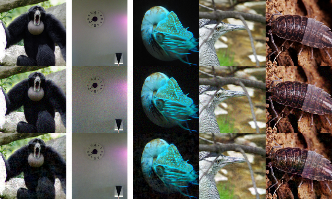
Several adversarial images, crafted by the baseline method and the spanning attack, are displayed in Figure 4. All these adversarial images does not show any significant difference from the original images due to the fact that they have the same constraint on the perturbation norm.
Comments on improvement of success rates.
The black-box attack is a non-convex zeroth-order optimization problem; there is always a chance that the baseline method is trapped in some local areas, and as a consequence fails to attack. For instance, when RGF estimates gradients, informative random vectors could be too sparse to find an accurate gradient, as these random vectors are sampled from a large space. In contrast, the spanning attack employs prior knowledge (encoded in the subspace) about adversarial perturbations, and hence reduces the possibility of being trapped. That’s why the spanning attack could improve success rates and query efficiency simultaneously. It is noteworthy that the capability of the spanning attack depends on the subspace dataset (the prior knowledge encoded); we will carefully investigate it in the next section.
Since the results are consistent across all baseline methods and target models, in the following we take the RGF attack against ResNet-50 as illustration by default to avoid unnecessary repetition.
5.2 Investigation on the subspace
In this section, we study to what extent the subspace impacts on the performance of the spanning attack, and furthermore how we could establish the subspace dataset in practice.
5.2.1 Size of the subspace dataset
We show attack performance with different sizes of the subspace dataset in Figure 5. (We will talk about TRS in Section 5.2.2.) In our experiments, the minimum size is 100 and the maximum size is 1,000. In this scope, the larger the subspace size, the better the performance of the spanning attack. In contrast, the baseline method is the extreme case where the subspace size is . Therefore, it is expected that the performance of the spanning attack will reach the peak and then slide down as the subspace size increases. It is noteworthy that even a small subspace dataset, as shown in Figure 5, would help the spanning attack defeat the baseline methods.
5.2.2 Distribution of the subspace dataset
| Success rate | Query mean | Query median | |
| Baseline | 0.971 | 589.575 | 358.0 |
| Spanning attack | 0.991 | 329.541 | 205.0 |
| Spanning attack (label biased) | 0.991 | 316.572 | 205.0 |
| Spanning attack (Flickr8k) | 0.990 | 318.333 | 205.0 |
| Spanning attack (TRS) | 0.960 | 654.491 | 358.0 |
| Bottom spanning attack | 0.991 | 298.817 | 154.0 |
| Top spanning attack | 0.991 | 354.346 | 205.0 |
We investigate whether it is necessary to sample the subspace dataset from the same distribution as the training data. Specifically, we further try three settings for the subspace dataset:
- •
1) instances of top 50 classes from the ImageNet validation set. Note that there are 1,000 classes in total, and hence it is a label-biased setting.
- •
2) instances from the Flickr8k dataset (Hodosh et al. 2015), which is much different from the ImageNet dataset.
- •
3) instances sampled from a uniform distribution. In other words, the spanned subspace could be seen as a totally random subspace (TRS) without any prior knowledge.
The results are displayed in the middle area of Table 2. On the one hand, the results of the label-biased and the Flickr8k spanning attack are still better than the baseline, and competitive with the spanning attack in Section 5.1 (see the upper area of Table 2 for convenience), where the subspace dataset is sampled i.i.d. (without any bias) from the ImageNet validation set. It suggests that even a biased subspace dataset suffices to work, which extends the application range of the spanning attack. In a word, the subspace dataset does not necessarily has to be sampled from the same distribution with the training data.
On the other hand, the spanning attack with a totally random subspace performs even worse than the baseline. (To better illustrate this issue, we also show attack performance for different subspace sizes with totally random subspaces in Figure 5.) In other words, the totally random subspace plays a negative role on performance. The result validates that prior knowledge given by the subspace dataset is necessary, rather than an arbitrary low-dimensional subspace.
Discussion on establishing the subspace dataset in practice.
The experimental results of Section 5.2.1 and Section 5.2.2 jointly suggest that the conditions which the subspace dataset has to obtain is not too strict in practice: the size of the subspace dataset could be very small, and the distribution of the subspace could be different from the one of the training data. Therefore, when applying the subspace attack method in real-world applications, we only need to collect a small set of unlabeled data related to the target model. For instance, if the task is attacking a face recognition system, one possibility is to crawl the web and find some face pictures in advance.
5.2.3 Bottom and top spanning attack
We investigate whether the selective spanning attack could further improve performance. In our experiments, the bottom 800 singular vectors (remember the total number of the singular vectors is 1,000) are used for the bottom spanning attack, and the top 800 singular vectors are used for the top spanning attack. The comparison among the original spanning attack, bottom spanning attack and top spanning attack are shown in the lower area of Table 2. The results show that the bottom spanning attack could further improve performance, whereas the top spanning attack has a negative impact. This is an empirical validation that adversarial perturbations are more likely to appear in directions out of the data manifold, rather than along the data manifold, as discussed in Section 4.3.
5.3 Sensitivity to radii
We investigate whether the given radius affects the capability of the spanning attack over the baseline method. We report success rates, query means and query medians with varying radii. The results are illustrated in Figure 6, and show that the spanning attack improves the baseline method consistently across different radii. Note that in all the other experiments the radius is set .
5.4 More discussion with related work
Although the work of Yan et al. 2019 has a setting different from ours as discussed in Section 2, for completeness we try to adapt their methods for comparison. They require an auxiliary labeled dataset, focus on norm and only considers the soft-label black-box attack. In order to have a comparison, we let the subspace dataset be labeled with size 1,000. We notice that with such a small subspace dataset in our setting, Yan et al. 2019’s method does not perform well. For instance, when attacking ResNet-50, it has the success rate 58.7% and the query mean 641.283. The results for attacking VGG-16 and DenseNet-121 are similar (VGG-16: success rate 68.6%, query mean 558.044; DenseNet-121: success rate 59%, query mean 623.603). It is primarily due to the fact that their method trains substitute models with labeled data. As a consequence, when the dataset is too small, it is difficult to train reliable substitute models.
6 Conclusion
We propose a general technique named the spanning attack to improve efficiency of black-box attacks. The spanning attack is motivated by the theoretical analysis that minimum adversarial perturbations of machine learning models incline to be in the subspace of the training data. In practice, the spanning attack only requires a small auxiliary unlabeled dataset, and is applicable to a wide range of black-box attacks including both the soft-label black-box attacks and hard-label black-box attacks. Our experiments show that the spanning attack can significantly improve the query efficiency and success rates of black-box attacks simultaneously.
References
- Biggio and Roli (2018) Battista Biggio and Fabio Roli. Wild patterns: Ten years after the rise of adversarial machine learning. Pattern Recognition, 84:317–331, 2018.
- Brendel et al. (2018) Wieland Brendel, Jonas Rauber, and Matthias Bethge. Decision-based adversarial attacks: Reliable attacks against black-box machine learning models. In International Conference on Learning Representations (ICLR), 2018.
- Brunner et al. (2018) Thomas Brunner, Frederik Diehl, Michael Truong-Le, and Alois Knoll. Guessing smart: Biased sampling for efficient black-box adversarial attacks. In IEEE International Conference on Computer Vision (ICCV), pages 4958–4966, 2018.
- Carlini and Wagner (2017) Nicholas Carlini and David Wagner. Towards evaluating the robustness of neural networks. In IEEE Symposium on Security and Privacy (SP), pages 39–57, 2017.
- Chen et al. (2019) Hongge Chen, Huan Zhang, Duane Boning, and Cho-Jui Hsieh. Robust decision trees against adversarial examples. In International Conference on Machine Learning (ICML), pages 1122–1131, 2019.
- Chen et al. (2019) Jianbo Chen, Michael I. Jordan, and Martin J. Wainwright. Hopskipjumpattack: A query-efficient decision-based attack. CoRR, abs/1904.02144, 2019.
- Chen et al. (2017) Pin-Yu Chen, Huan Zhang, Yash Sharma, Jinfeng Yi, and Cho-Jui Hsieh. ZOO: Zeroth order optimization based black-box attacks to deep neural networks without training substitute models. In ACM Conference on Computer and Communications Security (CCS) Workshop on Artificial Intelligence and Security (AISec), pages 15–26, 2017.
- Cheney and Kincaid (2010) Ward Cheney and David R. Kincaid. Linear Algebra: Theory and Applications. The Saylor Foundation, 2010.
- Cheng et al. (2019) Minhao Cheng, Thong Le, Pin-Yu Chen, Jinfeng Yi, Huan Zhang, and Cho-Jui Hsieh. Query-efficient hard-label black-box attack: An optimization-based approach. In International Conference on Learning Representations (ICLR), 2019.
- Cheng et al. (2020) Minhao Cheng, Simranjit Singh, Pin-Yu Chen, Sijia Liu, and Cho-Jui Hsieh. Sign-opt: A query-efficient hard-label adversarial attack. In International Conference on Learning Representations (ICLR), 2020.
- Cheng et al. (2019) Shuyu Cheng, Yinpeng Dong, Tianyu Pang, Hang Su, and Jun Zhu. Improving black-box adversarial attacks with a transfer-based prior. In Advances in Neural Information Processing Systems (NeurIPS), 2019.
- Cortes and Vapnik (1995) Corinna Cortes and Vladimir Vapnik. Support-vector networks. Machine Learning, 20(3):273–297, 1995.
- Deng et al. (2009) Jun Deng, Wenjie Dong, Richard Socher, Li-Jia Li, Kehui Li, and Li Fei-Fei. Imagenet: A large-scale hierarchical image database. In IEEE Conference on Computer Vision and Pattern Recognition (CVPR), pages 248–255, 2009.
- Fawzi et al. (2018) Alhussein Fawzi, Omar Fawzi, and Pascal Frossard. Analysis of classifiers’ robustness to adversarial perturbations. Machine Learning, 107(3):481–508, 2018.
- Goodfellow et al. (2015) Ian J. Goodfellow, Jonathon Shlens, and Christian Szegedy. Explaining and harnessing adversarial examples. In International Conference on Learning Representations (ICLR), 2015.
- He et al. (2016) Kaiming He, Xiangyu Zhang, Shaoqing Ren, and Jian Sun. Deep residual learning for image recognition. In IEEE Conference on Computer Vision and Pattern Recognition (CVPR), pages 770–778, 2016.
- Hodosh et al. (2015) Micah Hodosh, Peter Young, and Julia Constanze Hockenmaier. Framing image description as a ranking task: data, models and evaluation metrics. In International Conference on Artificial Intelligence (IJCAI), pages 4188–4192, 2015.
- Huang et al. (2017) Gao Huang, Zhuang Liu, Laurens van der Maaten, and Kilian Q. Weinberger. Densely connected convolutional networks. In IEEE Conference on Computer Vision and Pattern Recognition (CVPR), pages 2261–2269, 2017.
- Ilyas et al. (2018) Andrew Ilyas, Logan Engstrom, Anish Athalye, and Jessy Lin. Black-box adversarial attacks with limited queries and information. In International Conference on Machine Learning (ICML), pages 2142–2151, 2018.
- Ilyas et al. (2019) Andrew Ilyas, Logan Engstrom, and Aleksander Madry. Prior convictions: Black-box adversarial attacks with bandits and priors. In International Conference on Learning Representations (ICLR), 2019.
- Kantchelian et al. (2016) Alex Kantchelian, JD Tygar, and Anthony Joseph. Evasion and hardening of tree ensemble classifiers. In International Conference on Machine Learning (ICML), pages 2387–2396, 2016.
- Katz et al. (2017) Guy Katz, Clark Barrett, David L Dill, Kyle Julian, and Mykel J Kochenderfer. Reluplex: An efficient SMT solver for verifying deep neural networks. In International Conference on Computer Aided Verification, pages 97–117, 2017.
- Liu et al. (2019) Sijia Liu, Pin-Yu Chen, Xiangyi Chen, and Mingyi Hong. signsgd via zeroth-order oracle. In International Conference on Learning Representations (ICLR), 2019.
- Liu et al. (2017) Yanpei Liu, Xinyun Chen, Chang Liu, and Dawn Song. Delving into transferable adversarial examples and black-box attacks. In International Conference on Learning Representations (ICLR), 2017.
- Madry et al. (2018) Aleksander Madry, Aleksandar Makelov, Ludwig Schmidt, Dimitris Tsipras, and Adrian Vladu. Towards deep learning models resistant to adversarial attacks. In International Conference on Learning Representations (ICLR), 2018.
- Nesterov and Spokoiny (2017) Yurii Nesterov and Vladimir G. Spokoiny. Random gradient-free minimization of convex functions. Foundations of Computational Mathematics, 17(2):527–566, 2017.
- Papernot et al. (2016) Nicolas Papernot, Patrick D. McDaniel, and Ian J. Goodfellow. Transferability in machine learning: from phenomena to black-box attacks using adversarial samples. CoRR, abs/1605.07277, 2016.
- Papernot et al. (2017) Nicolas Papernot, Patrick McDaniel, Ian Goodfellow, Somesh Jha, Z. Berkay Celik, and Ananthram Swami. Practical black-box attacks against machine learning. In Asia Conference on Computer and Communications Security, pages 506–519, 2017.
- Simonyan and Zisserman (2015) Karen Simonyan and Andrew Zisserman. Very deep convolutional networks for large-scale image recognition. In International Conference on Learning Representations (ICLR), 2015.
- Steiner et al. (2019) Benoit Steiner, Zachary DeVito, Soumith Chintala, Sam Gross, Adam Paszke, Francisco Massa, Adam Lerer, Gregory Chanan, Zeming Lin, Edward Yang, Alban Desmaison, Alykhan Tejani, Andreas Kopf, James Bradbury, Luca Antiga, Martin Raison, Natalia Gimelshein, Sasank Chilamkurthy, Trevor Killeen, Lu Fang, and Junjie Bai. Pytorch: An imperative style, high-performance deep learning library. In Advances in Neural Information Processing Systems (NeurIPS), pages 8024–8035, 2019.
- Stutz et al. (2019) David Stutz, Matthias Hein, and Bernt Schiele. Disentangling adversarial robustness and generalization. In IEEE Conference on Computer Vision and Pattern Recognition (CVPR), pages 6976–6987, 2019.
- Su et al. (2018) Dong Su, Huan Zhang, Hongge Chen, Jinfeng Yi, Pin-Yu Chen, and Yupeng Gao. Is robustness the cost of accuracy? – a comprehensive study on the robustness of 18 deep image classification models. In European Conference on Computer Vision (ECCV), pages 644–661, 2018.
- Szegedy et al. (2014) Christian Szegedy, Wojciech Zaremba, Ilya Sutskever, Joan Bruna, Dumitru Erhan, Ian J. Goodfellow, and Rob Fergus. Intriguing properties of neural networks. In International Conference on Learning Representations (ICLR), 2014.
- Tu et al. (2019) Chun-Chen Tu, Paishun Ting, Pin-Yu Chen, Sijia Liu, Huan Zhang, Jinfeng Yi, Cho-Jui Hsieh, and Shin-Ming Cheng. Autozoom: Autoencoder-based zeroth order optimization method for attacking black-box neural networks. In AAAI Conference on Artificial Intelligence (AAAI), volume 33, pages 742–749, 2019.
- Uesato et al. (2018) Jonathan Uesato, Brendan O’Donoghue, Pushmeet Kohli, and Aäron van den Oord. Adversarial risk and the dangers of evaluating against weak attacks. In International Conference on Machine Learning (ICML), pages 5025–5034, 2018.
- Wang et al. (2019) Lu Wang, Xuanqing Liu, Jinfeng Yi, Zhi-Hua Zhou, and Cho-Jui Hsieh. Evaluating the robustness of nearest neighbor classifiers: A primal-dual perspective. CoRR, abs/1906.03972, 2019.
- Wang et al. (2020) Lu Wang, Xuanqing Liu, Jinfeng Yi, Yuan Jiang, and Cho-Jui Hsieh. Provably robust metric learning. In Advances in Neural Information Processing Systems (NeurIPS), 2020.
- Wang et al. (2017) Yining Wang, Simon S. Du, Sivaraman Balakrishnan, and Aarti Singh. Stochastic zeroth-order optimization in high dimensions. In International Conference on Artificial Intelligence and Statistics (AISTATS), pages 1356–1365, 2017.
- Yan et al. (2019) Ziang Yan, Yiwen Guo, and Changshui Zhang. Subspace attack: Exploiting promising subspaces for query-efficient black-box attacks. In Advances in Neural Information Processing Systems (NeurIPS), 2019.