Charged particle motion around non-singular black holes in conformal gravity in the presence of external magnetic field
Abstract
We consider electromagnetic fields and charged particle dynamics around non-singular black holes in conformal gravity immersed in an external, asymptotically uniform magnetic field. First, we obtain analytic solutions of the electromagnetic field equation around rotating non-singular black holes in conformal gravity. We show that the radial components of the electric and magnetic fields increase with the increase of the parameters and of the black hole solution. Second, we study the dynamics of charged particles. We show that the increase of the values of the parameters and and of magnetic field causes a decrease in the radius of the innermost stable circular orbits (ISCO) and the magnetic coupling parameter can mimic the effect of conformal gravity giving the same ISCO radius up to when .
pacs
04.70.Bw, 04.20.DwI Introduction
General Relativity has a good success in predicting and describing a number of observations and experiments about gravity. The recent detection of gravitational waves Abbott et al. 2016 and observation of black hole shadow Akiyama et al. 2019a can also be considered tests of General Relativity Akiyama et al. 2019b; The LIGO Scientific Collaboration and the Virgo Collaboration 2016, which successfully passed them. However, the theory itself is plagued by the problem of singularities. Most physically-relevant solutions of Einstein’s equation possess a singular region. The current standard understanding of physical laws cannot accept a singularity and there are several attempts to resolve the singularity problem (see, e.g., Bardeen 1968; Hayward 2006; Ayón-Beato and García 1998; Ayon-Beato 1999; Ayon-Beato and Garcia 1999; Fan and Wang 2016; Toshmatov et al. 2014; Englert et al. 1976; Narlikar and Kembhavi 1977; Mannheim 2012; Bars et al. 2014; Bambi 2013; Bambi et al. 2017; Bambi et al. 2016; Hořava 2009a; Hořava 2009b; Kehagias and Sfetsos 2009).
One of the examples to resolve the singularity problem has been proposed in Refs. Bambi et al. 2017, where, within a large class of conformally invariant theories of gravity, singularity-free black hole solutions have been proposed. The proposed spacetimes are geodetically complete and the curvature invariants do not diverge at .
Ref. Turimov et al. 2018 has been devoted to study the electromagnetic field around compact starts in conformal gravity. Using X-ray observations of supermassive black holes (SMBHs), it was proposed a test of conformal gravity in Zhou et al. 2018. The energy condition and scalar perturbations of the spacetime in conformal gravity have been studied in Toshmatov et al. 2017a; Toshmatov et al. 2017b. Recently, magnetized particle motion around black holes in conformal gravity in the presence of external magnetic fields has been studied in Haydarov et al. 2020. In this work, we plan to investigate charged particle motion acceleration around singularity-free black holes immersed in an external magnetic field.
A black hole itself cannot have its own magnetic field. However the curved spacetime will change the structure of electromagnetic field surrounding the black hole. The pioneer work of Wald has been devoted to study the electromagnetic field around a Kerr black hole immersed in an external, asymptotically uniform magnetic field Wald 1974. A number of works have been devoted to study the electromagnetic field and charged particle motion around compact objects in external magnetic fields Aliev et al. 1986; Aliev and Gal’tsov 1989; Aliev and Özdemir 2002; Frolov and Krtouš 2011; Frolov 2012; Benavides-Gallego et al. 2019; Shaymatov et al. 2018; Oteev et al. 2016; Toshmatov et al. 2015; Stuchlík et al. 2014; Abdujabbarov et al. 2014; Abdujabbarov and Ahmedov 2010; Abdujabbarov et al. 2011a; Abdujabbarov et al. 2011b; Abdujabbarov et al. 2008; Karas et al. 2012; Stuchlík and Kološ 2016; Kovář et al. 2010; Kovář et al. 2014; Kološ et al. 2017; Rayimbaev 2016; Rahimov et al. 2011; Rahimov 2011; Haydarov et al. 2020; Rayimbaev et al. 2020; Narzilloev et al. 2019.
The energetic process around black holes can be used to model the observational features of astrophysical objects (Relativistic jets, Soft gamma ray repeaters - SGR and etc.). Different mechanisms of energy extraction from black holes have been proposed: Penrose process Penrose 1969, Blandford-Znajeck mechanism Blandford and Znajek 1977, Magnetic Penrose process Dhurandhar and Dadhich 1983; Dhurandhar and Dadhich 1984a; Dhurandhar and Dadhich 1984b; Wagh et al. 1985, and particle acceleration mechanism (BSW) Bañados et al. 2009. Particularly, in Ref. Bañados et al. 2009 it was shown that the center of mass energy of colliding particles near an extreme rotating Kerr black hole may diverge for the fine tuned values of the angular momentum of the particles. Magnetic fields may play an important role in the charged particle acceleration near black holes Frolov and Krtouš 2011; Frolov 2012. Thus we are also interested to study the effects of conformal gravity and magnetic fields on the charged particle acceleration process.
In this paper, we study the dynamics of charged particles around black holes in conformal gravity in the presence of magnetic fields. The paper is organized as follows: Sect. II is devoted to study the electromagnetic field around black holes in conformal gravity immersed in an external, asymptotically uniform magnetic field. The charged particle motion around non-rotating and rotating black holes in conformal gravity in the presence of an external magnetic field has been studied in Sects. III and IV, respectively. In Sect. V, we study the collision of charged particles near a black hole in conformal gravity. We summarize our results in Sect. VI. Throughout this work, we use for the space-time signature and a system of units where .
II Electromagnetic field around a singularity free Black hole
In this section, we study the electromagnetic field around a singularity-free black hole in conformal gravity described by the line element
| (1) |
where
| (2) |
with
| (3) | |||||
and
| (4) |
where is the spin parameter of the black hole with total mass , is called the conformal rescaling, and and are conformal parameters; that is, parameters related to the conformal rescaling.
The Penrose diagram, and thus the causal structure of the spacetime, of our singularity-free black hole solution is the same as the Penrose diagram of the Kerr solution, because conformal transformations do not alter the causal structure of spacetimes. They only change distances. The Kerr singularity at is not a curvature singularity any longer in our solution, and this is possible because the scalar curvature and the Kretschmann scalar are not invariant under conformal trasformations. After the conformal rescaling, massive particles need an infinite time to reach the point . Massless particles require an infinite value of their affine parameter to reach the point . So the point is not a singularity in the sense of geodesic motion any longer either. The conformal rescaling has thus the capability to remove the Kerr singularity at . is also singular at and this is strictly necessary to compensate the singularity of the Kerr solution at . For , the conformal factor can remove the singularity of the Kerr metric at , while, for a lower value, the singularity of is not strong enough to compensate the singularity of the Kerr metric. More details can be found in the original paper deriving this solution Bambi et al. 2017
We start with considering the electromagnetic field around a singularity-free black hole immersed in an external, asymptotically uniform magnetic field aligned along the direction of the axis of symmetry of the space-time. The energy momentum tensor of the electromagnetic field is assumed to be negligibly small, does not change the spacetime metric, and is of the following order of magnitude
| (5) |
Using a Killing vector being responsible for the symmetry of spacetime geometry of the black hole, one may recall the equation
| (6) |
Expressions (6) can be used to have the following equation
| (7) |
where the Riemann curvature tensor can be transformed to the Ricci one in the following way
| (8) |
For the spacetime of the singularity free rotating black hole in the conformal gravity, the right hand side of Eq. (8) can be chosen as . The Maxwell equations then can be expressed in the following form
| (9) |
where is electromagnetic field tensor and can be selected as
| (10) |
Here is an integration constant and the 4-vector is a correction to the potential due to the presence of the conformal gravity parameters responsible for the Ricci non flatness of the spacetime. The 4-vector can be found from the equation .
The electromagnetic potential then can be written as the sum of two contributions
| (11) |
where is the potential being proportional to the Killing vectors. To find the solution for , one can use the ansatz for the vector potential of the electromagnetic field in the Lorentz gauge in the form Wald 1974. The constant , where the gravitational source is immersed in a uniform magnetic field B being parallel to its axis of rotation. The value of the remaining constant can be easily calculated from the asymptotic properties of the spacetime (2) at the asymptotical infinity.
The second part of the total vector potential of the electromagnetic field is produced due to the contribution of conformal gravity and has the following solution , where the expression for the constant can be easily found from the asymptotic properties of the spacetime (2) at infinity Abdujabbarov et al. 2008; Abdujabbarov and Ahmedov 2010. However, since the effect of conformal gravity is negligibly small at large distances, one might exclude this part tending and use the traditional contravariant expression for the 4-vector potential as in the Kerr case.
Finally, the components of the 4-vector potential of the electromagnetic field will take a form
| (12) | |||||
| (13) | |||||
| (14) | |||||
| (15) | |||||
where, for simplicity, we take . The components of the electric and magnetic fields in the frame moving with four velocity read
| (16) | |||||
| (17) |
where the electromagnetic field tensor, , in terms of the four potential can be expressed as
| (18) |
Using the the expressions above for the zero angular momentum observers (ZAMO) with the four-velocity components
| (19) | |||||
one can easily find the components of the electromagnetic field using the expressions in (16)-(18). The nonvanishing orthonormal components of the electromagnetic field measured by zero angular momentum observers with the four-velocity that has the form (19) are given by the expressions in (44)-(47) and linear approximation of conformal gravity parameter is presented by the expressions in (48)-(51) in appendix A.
Fig. 1 shows the radial dependence of the components of electromagnetic fields in the cases of different values of the angle and conformal gravity parameter . Since the expressions in (44)-(47) have a complex form, one might be interesting to see the structure of the electromagnetic fields around BHs in the ZAMO frame, which is presented in Fig. 2.
a. b.
In the case of slow rotation () and far distance (), expressions (44)-(47) reduce to
| (20) | |||||
| (21) | |||||
| (22) | |||||
| (23) | |||||
From the expressions in (20)-(23), one can see that in such limits only the components and are affected by conformal gravity while other components ( and ) do not include any contribution from (for the chosen approximation). The latter is especially clearly seen for in the graphs presented in Fig. 1. In the limit of flat spacetime, i.e. for , and , expressions (44)–(47) give the following limiting expressions: , being consistent with the solutions for the homogeneous magnetic field in Newtonian limit.
Figure 3 presents the profiles of magnetic fields around black holes for different values of spin and conformal parameter. One can see from the right top and bottom panels that the conformal parameter forces the parallel field line to have a dipole-like structure. Finally, bottom panels give the possibilities of the comparison of the nature of conformal and spin parameters of the black hole.
III Charged particle motion around a Conformal non-rotating black hole immersed in a uniform magnetic field
Here we study charged particle motion around a black hole in conformal gravity in the presence of an external, uniform magnetic field. The Hamilton-Jacobi equation for a test particle with mass and charge can be written as
| (24) |
The solution of equation (24) can be sought in the following form
| (25) |
where and are the specific energy and the specific angular momentum of the test particle, respectively.
It is convenient to consider the particle motion on the equatorial plane plane, where (). Then we can write
| (26) |
where the effective potential has a form
| (27) |
and is the magnetic coupling parameter, or the so-called cyclotron frequency, which characterizes the interaction between the charged particle and the magnetic field. The effective potential is invariant under the following transformations: , where the Lorentz force acting on the charged particle is repulsive and has the same direction as the centrifugal force, and , where the Lorentz force is attractive and has the same direction as the gravitational force. Below we analyze the effective potential (27) for positive angular momenta of the particle and either positive or negative magnetic coupling parameter.
Fig. 4 shows the radial dependence of the effective potential on the equatorial plane. One can see from Fig. 4 that when the effective potential is higher than in the case and increases with the increase of the values of parameters and . It is worth to note that at large distances the effect of the magnetic field plays a more important role than the effect of conformal gravity.
III.1 Stable Circular orbits
Now we will consider the innermost stable circular orbits of charged particles using following the standard conditions
| (28) |
In fact, circular orbits can be stable when the second derivative of the effective potential with respect to both coordinates ( and ) is positive and the ISCO on the equatorial plane corresponds to the zero value of this derivative . The angular momentum of circular orbits can be found in the following form
| (29) |
In order to ensure that we obtain a real solution of equation (III.1), we require the function under the square root to be always positive. Since the second part of the equation under the square root is always positive, it implies
| (30) |
must be satisfied for any values of and .
Now we will analyze the distance where is always positive i.e. positions where circular motion can occurs in the equatorial plane.
Fig. 5 illustrates the dependence of the minimum distance where circular orbits are allowed from the cyclotron frequency for the different values of the conformal parameters and . One can see from the figure that independently from the values of and such minimum orbits starts from the value in the absence of external magnetic field and then decreases with the increase of the latter one. It is also worth to note that the rate of such decrease reduces with the increase of both conformal parameters.
Fig. 6 shows the radial dependence of the critical value of the angular momentum for circular orbits. One can see from this figure that the value of the critical angular momentum of the charged particle increases in the presence of an external magnetic field.
The energy of the charged particle at circular orbits can be obtained substituting Eq. (III.1) into Eq. (27)
| (31) |
Here we will study radial dependence of the energy in the equatorial plane, where .
Fig. 7 illustrates the radial profiles of the charged particle energy in circular orbits on the equatorial plane. One can see that the magnetic field increases the energy of the charged particle. One more thing is that the rate of energy increase in the case of is higher than the case of .
In Fig. 8, we present the effect of conformal gravity and magnetic field on the ISCO radius of charged particles. One can see from the figure that increasing the conformal parameters and and the magnetic coupling parameter decreases of the ISCO radius.
In Fig. 9 it is illustrated the dependence of ISCO radius of neutral (first panel) and charged (second panel) particles on the conformal parameter , for the chosen values of the parameter . One can see from the first panel that the minimum values of the ISCO radius tends to for the neutral particles independently from the parameter , while for the charged ones this minimum ISCO radius decreases with the increase of .
III.2 Charged particles trajectories
Now we will study the effects of the parameters of conformal gravity on the trajectories of charged particles.
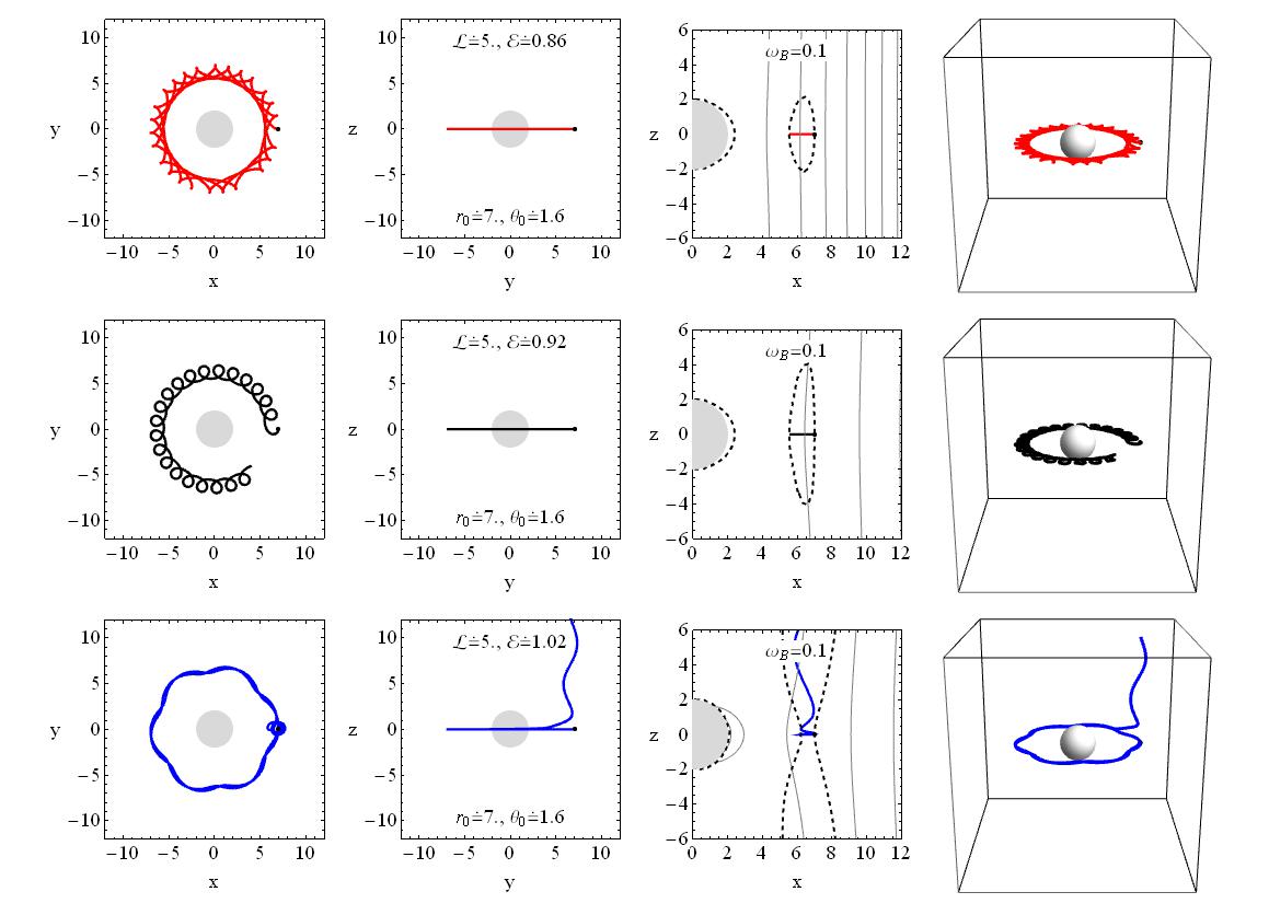

Trajectories of positive and negative charged particles for absolute values of the magnetic coupling parameter are shown in Fig. 10. All plots in this figure are taken at the value of the conformal parameter and trajectories of the charged particles in red lines on first and fourth rows correspond to the values of the conformal parameters , black and blue lines correspond to the conformal parameter and , respectively for the fixed value of the specific angular momentum . One can see from the figures that the specific energy of the charged particles increases with increasing of the conformal parameter . Moreover, the orbits of charged particles started at equatorial plane become unstable and the particle leaves the central object at higher values of . It can be explained by the magnetic field structure around the black hole in conformal gravity which is shown in the third column of the plots in grey lines that becomes dipol like structure at the higher values of the parameter .
III.3 Conformal non-rotating black hole versus Schwarzschild black hole in a uniform magnetic field
In this subsection, we consider two different cases: the motion of a charged particle around a Schwarzschild black hole and a non-rotating black hole in conformal gravity, in a magnetic field, with the same ISCO radius for the charged particle.
Fig. 12 show that the impact of the conformal parameter and of the magnetic coupling parameter on the ISCO radius is the same.
Fig. 13 shows the relation between the conformal and magnetic coupling parameters and , for the same ISCO radius. One can see from this figure that a magnetic field can mimic conformal gravity for the values of the parameter and the other conformal parameter at , and , respectively.
IV Charged particle motion around Conformal rotating black holes immersed in a uniform magnetic field.
Since the spacetime of a rotating black hole in conformal gravity admits separation of variables on the equatorial plane () we will study the motion around the source described by the metric (1) using the Hamilton-Jacobi equation where the action can be decomposed in the form as Eq. (25). Finally we obtain the equation of motion in the following form (for ):
| (32) | |||||
| (33) | |||||
| (34) |
where
| (35) | |||||
One may define the effective potential in the following form
| (36) |
Radial dependence of the effective potential is presented in Fig. 14, where graphs a. and b. are plotted in the case when the values of the angular momentum and energy of the particle are chosen to be equal to the values of a particle moving around the innermost circular orbit so, turning points of the lines on the graphs represent the ISCO radius; while in c. the lines correspond to the case when energy and angular momentum of the test particle are fixed for the various values of rotation parameter of a black hole.
a. b. c.
The stability of the equatorial orbits can be checked by plotting the trajectories of charged particles for given values of the external magnetic field and the conformal parameter as illustrated in Fig. 15 (the axis is assumed to be parallel to the symmetry axis and the origin coincides with the centre of the gravitating object). It is clearly seen from the second row of figures that for fixed values of the parameters mentioned the trajectory remains stable.
a.
 b.
b.
 c.
c.

The value of the ISCO radius can be obtained from the following standard conditions
| (37) | |||||
| (38) | |||||
| (39) |
with taking the form (35). The results of equations (37)-(39) are expressed in Fig. 16, panel a for a vanishing magnetic field and a non-vanishing spin parameter and panel b for a non-vanishing magnetic field and a vanishing spin parameter. We can clearly see from the figures that in the absence of an external magnetic field but non-vanishing spin parameter the ISCO radius first slightly increases for small values of the conformal parameter and then goes down for higher values of . In the case of a vanishing spin parameter but in the presence of an external magnetic field, it always monotonically decreases with the increase of the conformal parameter . In Tab. 1 and Tab. 2 numerical results in the presence of both rotation and magnetic parameters are presented. From the tables, one can see that for chosen values of the ISCO radius increases if one increases the conformal gravity parameter for a given interval of the latter one. The opposite scenario takes place for a given value of conformal parameter i.e. the increase of magnetic parameter decreases the ISCO radius. One should also mention that for the case of extreme rotation the ISCO radius becomes bigger compared to the case of pure Kerr metric where the ISCO becomes close to .
a. b.
| 0 | 0.001 | 0.002 | 0.005 | 0.01 | |
| 3.7312 | 3.7314 | 3.7316 | 3.7322 | 3.7331 | |
| 3.2897 | 3.2899 | 3.29 | 3.2904 | 3.2911 | |
| 2.8444 | 2.8445 | 2.8446 | 2.8449 | 2.8454 | |
| 2.4799 | 2.48 | 2.4801 | 2.4803 | 2.4807 | |
| 2.2192 | 2.2193 | 2.2194 | 2.2195 | 2.2197 |
| 0 | 0.001 | 0.002 | 0.005 | 0.01 | |
| 3.1458 | 3.1459 | 3.146 | 3.1462 | 3.1467 | |
| 3.1074 | 3.1075 | 3.1076 | 3.1078 | 3.1083 | |
| 3.0248 | 3.0249 | 3.025 | 3.0253 | 3.0257 | |
| 2.8316 | 2.83165 | 2.8317 | 2.832 | 2.8324 | |
| 2.2265 | 2.2267 | 2.2268 | 2.2273 | 2.2281 | |
| 1.4045 | 1.4049 | 1.4054 | 1.4067 | 1.4092 |
V Center-of-mass energy of charged particles collisions
In this section, we investigate the center-of-mass energy from collisions of two charged particles near rotating magnetized black holes in conformal gravity. The general expression for the center-of-mass energy for two particles coming from infinity with masses and and four-velocities and , respectively, can be found as the sum of their four-momenta Grib and Pavlov 2011a; Grib and Pavlov 2011b
| (40) |
Square of the center-of-mass energy can be defined in (40) and we have
| (41) |
after algebraic substitutions, we have the expression in a dimensionless form
| (42) |
Using the expression for the four velocities of the charged particles around magnetized rotating black holes in conformal gravity and considering the collision of the particles with equal mass and initial energy , one may get the expression for the center-of-mass energy in the following form
| (43) |
We analyze the center-of-mass energy of the collision of positive and positive (positive and negative) charged particles with the magnetic interaction parameter coming from infinity with initial energy and angular momentum .
The radial dependence of center-of-mass energy of collisions of positive-positive and positive-negative charged particles near a rotating black hole in an external magnetic field is shown in Figs. 17 and 18, for different values of the conformal and spin parameters. One can see from the figures that the center of mass energy decreases with the increase of the conformal parameter and spin parameter. Moreover, in the case of the collisions of positive-positive charged particles, the center of mass energy disappears due to dominated repulsive Coulomb forces. This implies that the collision does not occur at the point where the energy disappears. The distance where the center-of-mass energy disappears increases (decreases) increasing the conformal (spin) parameter.
VI Conclusion
In this work we have considered dynamics of charged particles and electromagnetic fields in the vicinity of rotating black holes in conformal gravity immersed in an external, asymptotically uniform magnetic field. The study of electromagnetic fields shows that the angular (radial) component of the magnetic field and the absolute value of the external magnetic field decrease (increases) with the increase of both parameters of conformal gravity, and , and the increase of the parameters of conformal gravity forces the external uniform magnetic field to have a dipole-like structure.
One may see from the studies of particle dynamics of charged particles around conformal non-rotating black holes in the presence of a magnetic field that the minimum circular orbits and ISCO radius decrease as with the increase of the conformal gravity and magnetic coupling parameters and in the case of rotating black holes the ISCO decreases faster. Moreover, it is shown that the particle orbits become unstable at higher values of both conformal parameter as a result of the fact that the magnetic field gets a dipole structure.
We have studied the effect of conformal gravity on the ISCO radius of charged particles around non-rotating black holes in the presence of an external magnetic field. We have shown that the conformal parameters can mimic the magnetic coupling parameters when (, ) at the values of conformal parameters (, ) while and with increasing of the value of the conformal parameter the mimic value of the coupling parameter increases.
The studies of center-of-mass energies of collisions of two charged particles show that the increase of both conformal and spin parameters causes a decrease in the center-of-mass energy.
Acknowledgments
This research is supported by the Uzbekistan Ministry for Innovative Development, Grants No. VA-FA-F-2-008 and No. MRB-AN-2019-29, the Innovation Program of the Shanghai Municipal Education Commission, Grant No. 2019-01-07-00-07-E00035, and the National Natural Science Foundation of China (NSFC), Grant No. 11973019. B.N. also acknowledges support from the China Scholarship Council (CSC), grant No. 2018DFH009013. This research is partially supported by an Erasmus+ exchange Grant between SU and NUUz. A.A. is supported by a postdoc fund through PIFI of the Chinese Academy of Sciences.
Appendix A Electromagnetic field components
| (44) | |||||
| (45) | |||||
| (46) | |||||
| (47) | |||||
where we used the following notations
and
| (48) | |||||
| (49) | |||||
| (50) | |||||
| (51) |
Here (hat) stands for orthonormal components of the electric and magnetic fields.
References
- Abbott et al. (2016) B. P. Abbott, R. Abbott, T. D. Abbott, M. R. Abernathy, F. Acernese, K. Ackley, C. Adams, T. Adams, P. Addesso, R. X. Adhikari, and et al., Physical Review Letters 116, 061102 (2016), arXiv:1602.03837 [gr-qc] .
- Akiyama et al. (2019a) K. Akiyama et al. (Event Horizon Telescope), Astrophys. J. 875, L1 (2019a).
- Akiyama et al. (2019b) K. Akiyama et al. (Event Horizon Telescope), Astrophys. J. 875, L6 (2019b).
- The LIGO Scientific Collaboration and the Virgo Collaboration (2016) The LIGO Scientific Collaboration and the Virgo Collaboration, Physical Review Letters 116, 241103 (2016), arXiv:1606.04855 [gr-qc] .
- Bardeen (1968) J. Bardeen, in Proceedings of GR5, edited by C. DeWitt and B. DeWitt, Tbilisi, USSR (Gordon and Breach, 1968) p. 174.
- Hayward (2006) S. A. Hayward, Physical Review Letters 96, 031103 (2006), gr-qc/0506126 .
- Ayón-Beato and García (1998) E. Ayón-Beato and A. García, Physical Review Letters 80, 5056 (1998), gr-qc/9911046 .
- Ayon-Beato (1999) E. Ayon-Beato, Physics Letters B 464, 25 (1999), hep-th/9911174 .
- Ayon-Beato and Garcia (1999) E. Ayon-Beato and A. Garcia, General Relativity and Gravitation 31, 629 (1999), gr-qc/9911084 .
- Fan and Wang (2016) Z.-Y. Fan and X. Wang, Phys. Rev. D 94, 124027 (2016), arXiv:1610.02636 [gr-qc] .
- Toshmatov et al. (2014) B. Toshmatov, B. Ahmedov, A. Abdujabbarov, and Z. Stuchlík, Phys. Rev. D. 89, 104017 (2014), arXiv:1404.6443 [gr-qc] .
- Englert et al. (1976) F. Englert, C. Truffin, and R. Gastmans, Nuclear Physics B 117, 407 (1976).
- Narlikar and Kembhavi (1977) J. V. Narlikar and A. K. Kembhavi, Nuovo Cimento Lettere 19, 517 (1977).
- Mannheim (2012) P. D. Mannheim, Foundations of Physics 42, 388 (2012), arXiv:1101.2186 [hep-th] .
- Bars et al. (2014) I. Bars, P. Steinhardt, and N. Turok, Phys. Rev. D 89, 043515 (2014), arXiv:1307.1848 [hep-th] .
- Bambi (2013) C. Bambi, Phys. Rev. D 87, 084039 (2013), arXiv:1303.0624 [gr-qc] .
- Bambi et al. (2017) C. Bambi, L. Modesto, and L. Rachwał, JCAP 5, 003 (2017), arXiv:1611.00865 [gr-qc] .
- Bambi et al. (2016) C. Bambi, D. Malafarina, and L. Modesto, Journal of High Energy Physics 2016, 147 (2016), arXiv:1603.09592 [gr-qc] .
- Hořava (2009a) P. Hořava, Phys. Rev. D 79, 084008 (2009a), arXiv:0901.3775 [hep-th] .
- Hořava (2009b) P. Hořava, Physical Review Letters 102, 161301 (2009b), arXiv:0902.3657 [hep-th] .
- Kehagias and Sfetsos (2009) A. Kehagias and K. Sfetsos, Physics Letters B 678, 123 (2009), arXiv:0905.0477 [hep-th] .
- Turimov et al. (2018) B. Turimov, B. Ahmedov, A. Abdujabbarov, and C. Bambi, Phys. Rev. D 97, 124005 (2018), arXiv:1805.00005 [gr-qc] .
- Zhou et al. (2018) M. Zhou, Z. Cao, A. Abdikamalov, D. Ayzenberg, C. Bambi, L. Modesto, and S. Nampalliwar, Phys. Rev. D 98, 024007 (2018), arXiv:1803.07849 [gr-qc] .
- Toshmatov et al. (2017a) B. Toshmatov, C. Bambi, B. Ahmedov, A. Abdujabbarov, and Z. Stuchlík, European Physical Journal C 77, 542 (2017a), arXiv:1702.06855 [gr-qc] .
- Toshmatov et al. (2017b) B. Toshmatov, C. Bambi, B. Ahmedov, Z. Stuchlík, and J. Schee, Phys. Rev. D 96, 064028 (2017b), arXiv:1705.03654 [gr-qc] .
- Haydarov et al. (2020) K. Haydarov, A. Abdujabbarov, J. Rayimbaev, and B. Ahmedov, Universe 6 (2020), 10.3390/universe6030044.
- Wald (1974) R. M. Wald, Phys. Rev. D. 10, 1680 (1974).
- Aliev et al. (1986) A. N. Aliev, D. V. Galtsov, and V. I. Petukhov, Astrophys. Space Sci. 124, 137 (1986).
- Aliev and Gal’tsov (1989) A. N. Aliev and D. V. Gal’tsov, Soviet Physics Uspekhi 32, 75 (1989).
- Aliev and Özdemir (2002) A. N. Aliev and N. Özdemir, Mon. Not. R. Astron. Soc. 336, 241 (2002), gr-qc/0208025 .
- Frolov and Krtouš (2011) V. P. Frolov and P. Krtouš, Phys. Rev. D 83, 024016 (2011), arXiv:1010.2266 [hep-th] .
- Frolov (2012) V. P. Frolov, Phys. Rev. D. 85, 024020 (2012), arXiv:1110.6274 [gr-qc] .
- Benavides-Gallego et al. (2019) C. A. Benavides-Gallego, A. Abdujabbarov, D. Malafarina, B. Ahmedov, and C. Bambi, Phys. Rev. D 99, 044012 (2019), arXiv:1812.04846 [gr-qc] .
- Shaymatov et al. (2018) S. Shaymatov, B. Ahmedov, Z. Stuchlík, and A. Abdujabbarov, International Journal of Modern Physics D 27, 1850088 (2018).
- Oteev et al. (2016) T. Oteev, A. Abdujabbarov, Z. Stuchlík, and B. Ahmedov, Astrophys. Space Sci. 361, 269 (2016).
- Toshmatov et al. (2015) B. Toshmatov, A. Abdujabbarov, B. Ahmedov, and Z. Stuchlík, Astrophys Space Sci 360, 19 (2015).
- Stuchlík et al. (2014) Z. Stuchlík, J. Schee, and A. Abdujabbarov, Phys. Rev. D 89, 104048 (2014).
- Abdujabbarov et al. (2014) A. Abdujabbarov, B. Ahmedov, O. Rahimov, and U. Salikhbaev, Physica Scripta 89, 084008 (2014).
- Abdujabbarov and Ahmedov (2010) A. Abdujabbarov and B. Ahmedov, Phys. Rev. D 81, 044022 (2010), arXiv:0905.2730 [gr-qc] .
- Abdujabbarov et al. (2011a) A. Abdujabbarov, B. Ahmedov, and A. Hakimov, Phys.Rev. D 83, 044053 (2011a), arXiv:1101.4741 [gr-qc] .
- Abdujabbarov et al. (2011b) A. A. Abdujabbarov, B. J. Ahmedov, S. R. Shaymatov, and A. S. Rakhmatov, Astrophys Space Sci 334, 237 (2011b), arXiv:1105.1910 [astro-ph.SR] .
- Abdujabbarov et al. (2008) A. A. Abdujabbarov, B. J. Ahmedov, and V. G. Kagramanova, General Relativity and Gravitation 40, 2515 (2008), arXiv:0802.4349 [gr-qc] .
- Karas et al. (2012) V. Karas, J. Kovar, O. Kopacek, Y. Kojima, P. Slany, and Z. Stuchlik, in American Astronomical Society Meeting Abstracts #220, American Astronomical Society Meeting Abstracts, Vol. 220 (2012) p. 430.07.
- Stuchlík and Kološ (2016) Z. Stuchlík and M. Kološ, European Physical Journal C 76, 32 (2016), arXiv:1511.02936 [gr-qc] .
- Kovář et al. (2010) J. Kovář, O. Kopáček, V. Karas, and Z. Stuchlík, Classical and Quantum Gravity 27, 135006 (2010), arXiv:1005.3270 [astro-ph.HE] .
- Kovář et al. (2014) J. Kovář, P. Slaný, C. Cremaschini, Z. Stuchlík, V. Karas, and A. Trova, Phys. Rev. D 90, 044029 (2014), arXiv:1409.0418 [gr-qc] .
- Kološ et al. (2017) M. Kološ, A. Tursunov, and Z. Stuchlík, Eur. Phys. J. C. 77, 860 (2017), arXiv:1707.02224 [astro-ph.HE] .
- Rayimbaev (2016) J. R. Rayimbaev, Astrophys Space Sc 361, 288 (2016).
- Rahimov et al. (2011) O. G. Rahimov, A. A. Abdujabbarov, and B. J. Ahmedov, Astrophysics and Space Science 335, 499 (2011), arXiv:1105.4543 [astro-ph.SR] .
- Rahimov (2011) O. G. Rahimov, Modern Physics Letters A 26, 399 (2011), arXiv:1012.1481 [gr-qc] .
- Haydarov et al. (2020) K. Haydarov, J. Rayimbaev, A. Abdujabbarov, S. Palvanov, and D. Begmatova, arXiv e-prints , arXiv:2004.14868 (2020), arXiv:arXiv:2004.14868 [gr-qc] .
- Rayimbaev et al. (2020) J. Rayimbaev, A. Abdujabbarov, B. Turimov, and F. Atamurotov, arXiv e-prints , arXiv:2004.10031 (2020), arXiv:2004.10031 [gr-qc] .
- Narzilloev et al. (2019) B. Narzilloev, A. Abdujabbarov, C. Bambi, and B. Ahmedov, Phys. Rev. D 99, 104009 (2019), arXiv:1902.03414 [gr-qc] .
- Penrose (1969) R. Penrose, Journal of Mathematical Physics 10, 38 (1969).
- Blandford and Znajek (1977) R. D. Blandford and R. L. Znajek, Mon. Not. Roy. Astron. Soc. 179, 433 (1977).
- Dhurandhar and Dadhich (1983) S. V. Dhurandhar and N. Dadhich, Bulletin of the Astronomical Society of India 11, 85 (1983).
- Dhurandhar and Dadhich (1984a) S. V. Dhurandhar and N. Dadhich, Phys. Rev. D 29, 2712 (1984a).
- Dhurandhar and Dadhich (1984b) S. V. Dhurandhar and N. Dadhich, Phys. Rev. D 30, 1625 (1984b).
- Wagh et al. (1985) S. M. Wagh, S. V. Dhurandhar, and N. Dadhich, Astrophys J. 290, 12 (1985).
- Bañados et al. (2009) M. Bañados, J. Silk, and S. M. West, Physical Review Letters 103, 111102 (2009).
- Grib and Pavlov (2011a) A. A. Grib and Y. V. Pavlov, Gravitation and Cosmology 17, 42 (2011a), arXiv:1010.2052 [gr-qc] .
- Grib and Pavlov (2011b) A. A. Grib and Y. V. Pavlov, Astroparticle Physics 34, 581 (2011b), arXiv:1001.0756 [gr-qc] .