Topological regularization with

information filtering networks

Tomaso Aste

Department of Computer Science, UCL, London, UK.

UCL Centre for Blockchain Technologies, UCL, London, UK.

Systemic Risk Centre, London School of Economics, London UK.

Keywords: Topological regularization; Information Filtering Networks; Complex Systems; Covariance selection; Sparse inverse covariance; Chow-Liu Trees; Sparse Expectation-Maximization; IFN regression

Abstract

A methodology to perform topological regularization via information filtering network is introduced. This methodology can be directly applied to covariance selection problem providing an instrument for sparse probabilistic modeling with both linear and non-linear multivariate probability distributions such as the elliptical and generalized hyperbolic families. It can also be directly implemented for $L_{0}$ -norm regularized multicollinear regression. In this paper, I describe in detail an application to sparse modeling with multivariate Student-t. A specific $L_{0}$ -norm regularized expectation-maximization likelihood maximization procedure is proposed for this sparse Student-t case. Examples with real data from stock prices log-returns and from artificially generated data demonstrate applicability, performances, and potentials of this methodology.

1 Introduction

Regularization is an important tool in machine learning to reduce the tendency of models to overfit the dataset on which they are trained and then underperform on new data. In data-driven modeling, regularization typically consists in adding a penalization term to the objective function in order to control for the complexity of the model with the aim of reducing overfitting. The idea was originally introduced by Tikhonov 1943 and since then it has permeated the field of inverse problems and machine learning. There are different possible regularizations depending on the form of the penalization. The original Tikhonov approach (also known as ridge regression) was introduced in the context of multicollinear regression and consisted in penalizing the sum-of-square loss function by adding the sum of square of the regression coefficients (the $L_{2}$ -norm) giving in this way preference to models with smaller coefficients. Other forms of penalization can of course be implemented and a particularly successful one uses of the $L_{1}$ -norm instead of the $L_{2}$ -norm and it was named ‘lasso’ by Tibshirani 1996. One of the consequences of the $L_{1}$ -norm penalization is to force certain coefficients to be set to zero producing therefore sparse models. Sparsity is extremely advantageous for interpretability because it reduces the number of variables involved in the model. When sparsity and interpretability are the objective, then one would aim to penalize the objective function directly with a $L_{0}$ -norm that introduces a cost for the number of coefficients in the model therefore directly penalizing denser models. An advantage of the $L_{0}$ -norm penalization is that the non-zero coefficients are not shrank in value allowing, in some cases, the use of local optimization methods. However, $L_{0}$ -norm regularization has been proven to be in general challenging. Indeed, exact optimization under $L_{0}$ -norm penalty is computationally intractable being non-differentiable and having a combinatorically large number of possible configurations to be explored.

In this paper I propose the use of information filtering networks (IFN) for $L_{0}$ -norm topological regularization. IFN are a class of networks originally introduced to extract and analyze the relevant ‘backbone’ structure of interrelations in complex systems comprising a large number of interacting elements (Tumminello et al. 2005). They have been shown to provide a meaningful characterization of the structure of many systems in different domains from finance (Tumminello et al. 2007; Aste et al. 2010; Pozzi et al. 2013; Musmeci et al. 2014; Musmeci et al. 2015; Procacci and Aste 2019), to psychology (Christensen et al. 2018; Christensen 2018) and biology (Song et al. 2008; Song et al. 2012). Recently Massara et al. 2017 have introduced a class of IFN, named Triangulated Maximally Filtered Graph (TMFG), that is chordal and therefore particularly suited for probabilistic inference modeling. TMFG networks are clique tree made with tetrahedra and they can be generated in a computationally efficient way. More recently (Massara and Aste 2018) the TMFG approach has been radically generalized to a vaster class of clique forests with cliques of arbitrary sizes. The algorithm was named Maximally Filtered Clique Forest (MFCF) and it uses a computationally efficient clique expansion algorithm that has the property of being topologically invariant ensuring that the construction preserves chordality. In Barfuss et al. 2016 a local-global procedure (LoGo) for probabilistic modeling was introduced using TMFG as Markov random fields. It was shown that in the multivariate normal case the inverse covariance is sparse and it has non-zero elements coinciding with the TMFG network edges. Such non-zero coefficients of the sparse inverse covariance can be computed from local inversions on the network structure. This methodology was proven to be extremely effective producing sparse models with larger likelihhod performances than lasso and with lower computational burden. Despite it was introduced for different purposes, the LoGo approach is a specific instance of topological $L_{0}$ -norm regularization.

The general problem that I am addressing in this paper can be formulated as a likelihood optimization under a topological constraint. In other words, the IFN is a Bayesian prior for the inference model and the posterior probability is optimized given that prior structure. This general problem is independent on the kind of prior inference network structure and on the kind of probability modeling. In this paper I will show that this problem can be solved for both multivariate normal and multivariate Student-t modeling given a clique-tree prior inference network structure generated with the MFCF method. I will also argue that this $L_{0}$ -norm regularization approach is applicable to the covariance selection problem and it can be therefore used for any modeling with multivariate elliptical distributions and multilinear regression problems. To the best of my knowledge the proof of topologically-constrained likelihood optimization for Student-t models is an original result that I obtain in this paper by extending the expectation-maximization (EM) procedure (Dempster et al. 1977; Bishop 2006) to this $L_{0}$ -norm regularized sparse model.

To demonstrate applicability, robustness and validity of this topological regularization methodology I perform a set of experiments using both synthetic and real data from financial equity prices. I generated sets of clique tree IFNs via the MFCF approach varying the maximum clique sizes to explore a range of different sparsities. The results show that there are optimal levels of sparsification for off-sample likelihood maximization.

The paper is organize as follows. In section 2 I describe the construction of information filtering networks. The topological regularization approach is presented in section . Examples of the application of this methodology to real and synthetic data are provided in Section 4. Conclusions and perspectives are provided in Section 5. Proof of theorems and methodological details are given in the appendixes.

2 Information filtering network learning

The structure of chordal IFN can be learned by using a clique expansion procedure as described in Massara and Aste 2018, where a clique forest is constructed starting from a seed structure and including vertices into the forest one by one accordingly with a given gain function. The resulting network is named MFCF. Such a clique forest network is made of a set of cliques $\mathcal{C}$ that are the ‘vertices’ in the clique-forest structure, the ‘edges’ of the clique-forest structure are instead a set $\mathcal{S}$ of separators that are cliques themselves with the property that by removing one of them the connected component becomes separated into two components. Clique forests are chordal graphs.

The MFCF network complexity can be constrained by limiting the minimum and maximum clique sizes. By increasing the clique sizes ones increases the number of edges in the network making it denser. The full network is retrieved when the minimum clique size equals the total number of vertices. Separators can be constrained to be unique between two cliques (multiplicity one) or to be utilizable more than once by more than two cliques (multiplicity larger than one). The simplest clique is the 2-clique that has two elements and it is an edge. MFCF networks with two cliques only are segments if separators have multiplicity one or they are maximum spanning threes when separators have arbitrary multiplicity. The TMFG is obtained when cliques have all size 4 (tetrahedra) and the separators can be used only once. The networks that I use in this paper have minimum clique size equal to 2 and a maximum clique sizes ranging between 2 to the total number of vertices.

The MFCF clique expansion algorithm requires a gain function that is used to decide the inclusion of a vertex into the clique tree in a recursive way. The choice of a convenient gain function is strictly related to the problem under investigation. The gain function that I use in this paper is the sum of the squares of the coefficients of the Kendall correlation matrix. This gain function is a good proxy for likelihood in a range of problems. This is a very simple gain function that lead to networks with all cliques with maximum size. Indeed, with this kind of additive gain the algorithm always gains by enlarging the clique, if allowed. I choose Kendall correlations because they describe dependency for a broader class of multivariate random variables than the Pearson’s correlations. They, are non-linear and have been proven to be effective in practical applications (Pozzi et al. 2013).

The IFN structure is learned before the maximum likelihood estimate of the model-parameters and it is passed to the optimization procedure as a Bayesian prior. This approach is analogous to the LoGo methodology introduced in Barfuss et al. 2016. However, here we apply it to non-normal models and this has important implications. Indeed, outside normal modeling the structure of the IFN graph does no longer represents conditional independence and the sparse probability distribution function no longer factorizes over the IFN clique and separator structure (see Lauritzen 1996 and Eq.12 in Appendix A for this factorization for the multivariate normal probability distribution function case).

3 Topological regularization with IFN

The problem is to find the model parameters that maximize likelihood for a given IFN. In this paper I address this issue for probabilistic modeling with densities belonging to the elliptical family and I report results for the multivariate normal and Student-t cases.

For the whole elliptical family the probability density function can be written as:

f(\mathbf{X}=\mathbf{x})=k_{p}\sqrt{|\mathbf{J}|}g(\mathbf{x},\boldsymbol{\mu},\mathbf{J}),

(1)

where $\boldsymbol{\mu}=\mathbb{E}(\mathbf{X})$ are the expected values of $\mathbf{X}$ and $\mathbf{J}$ is a positively defined matrix which coincides with the inverse covariance matrix when it is defined (Fang 2018).

The matrix $\mathbf{J}$ is the quantity I am sparsifying in this proposed $L_{0}$ -norm topological regularization. Specifically, only the diagonal $(\mathbf{J})_{i,i}$ and elements $(\mathbf{J})_{i,j}$ corresponding to edges in the IFN are allowed to be different from zero. Therefore, the problem becomes to compute the values of the non-zero elements of $\mathbf{J}$ that maximize likelihood. Hereafter, I report the solution for the multivariate normal and Student-t cases.

3.1 Sparse maximum likelihood solution for the multivariate normal

The log-likelihood for the multivariate normal distribution is

Definition 1 (Normal log-likelihood)

Given a set of observations $\mathbf{\hat{x}}(s)=(\hat{x}_{1}(s),...,\hat{x}_{p}(s))^{\mathsf{T}}$ with $s=1...q$ , the log-likelihood of the multivariate normal is

\ell(\boldsymbol{\mu},\mathbf{J})=\frac{q}{2}\log|\mathbf{J}|-\frac{1}{2}\sum_{s=1}^{q}d_{\mathbf{\hat{x}}(s)}^{2}-\frac{qp}{2}\log\pi.

(2)

where

Definition 2 (Mahalanobis distance)

The term

d_{\hat{\mathbf{x}}(s)}^{2}=(\mathbf{\hat{x}}(s)-\boldsymbol{\mu})^{\mathsf{T}}\mathbf{J}(\mathbf{\hat{x}}(s)-\boldsymbol{\mu}),

(3)

is the square of the Mahalanobis distance (Chandra et al. 1936).

Remark 3

The matrix $\mathbf{J}$ in Eqs.2 and 3 must be positively defined and sparse with non-zero elements only allowed on the diagonal and or in the off-diagonal positions coinciding with the edges of the associated IFN.

Now I must find the maximum likelihood solution of Eq.2 under the topological constraint that off-diagonal non-zero elements of $\mathbf{J}$ must coincide with the edges of the given IFN. The maximization process is almost identical to the full case but with the topological constraint enforced.

Theorem 4 (ML solution for $\boldsymbol{\mu}$ for the sparse multivariate normal problem)

If $\mathbf{J}$ is invertible, then the maximum likelihood solution for $\boldsymbol{\mu}$ is the sample mean:

\boldsymbol{\mu}^{*}=\frac{1}{q}\sum_{s=1}^{q}\mathbf{\hat{x}}(s)

(4)

Proof The proof is identical to the one for the full problem. The maximum of $\ell(\boldsymbol{\mu},\mathbf{J})$ in Eq.2 with respect to $\boldsymbol{\mu}$ is obtained from the root of

\frac{\partial}{\partial\boldsymbol{\mu}}\ell(\boldsymbol{\mu},\mathbf{J})=\frac{1}{2}\mathbf{J}\sum_{s=1}^{q}\mathbf{\hat{x}}(s)-\frac{q}{2}\mathbf{J}\boldsymbol{\mu}=0\;.

(5)

Which is indeed solved by $\boldsymbol{\mu}^{*}$ if $\mathbf{J}$ is invertible. $\square$

The proof that $\mathbf{J}$ is invertible is given in lemma 16 in Appendix B.

Theorem 5 (ML solution for $\mathbf{J}$ for the sparse multivariate normal problem)

Given a IFN structure made of clique and separators, the maximum likelihood solution for the sparse $\mathbf{J}$ is:

J^{*}_{i,j}=\sum_{c\in\mathcal{C}}\left(\hat{\boldsymbol{\Sigma}}_{c}^{-1}\right)_{i,j}-\sum_{s\in\mathcal{S}}\left(\hat{\boldsymbol{\Sigma}}_{s}^{-1}\right)_{i,j},

(6)

when $i,j$ belong to a clique of the IFN. Otherwise ${J^{*}}_{i,j}=0$ for all other couples of $i,j$ not belonging to cliques. Where $\hat{\boldsymbol{\Sigma}}_{c}$ and $\hat{\boldsymbol{\Sigma}}_{s}$ are the Person’s sample estimators of the covariances of the variables in the cliques and separators.
The proof of this theorem is provided in Appendix B.

Remark 6

The sparsification of $\mathbf{J}$ through Eq.6 provides a way to overcome the curse of dimensionality in the estimation of covariances from observations. Indeed, independently on the overall dimension of the system of variables $\mathbf{X}$ . When the sparse inverse covariance $\mathbf{J}$ is estimated from data, it is then sufficient to have a number of observations, $q$ , larger than the size of the largest clique, which is independent from the dimension, $p$ , of $\mathbf{X}$ . Therefore, through Eq.6 one can obtain well conditioned covariance matrices even when $q\ll p$ . Equation 6 transforms the global problem of estimating the whole matrix inverse into a set of local problems at clique and separator levels.

3.2 Sparse maximum likelihood solution for the multivariate Student-t

Definition 7 (Student-t log-likelihood)

Given a set of observations $\mathbf{\hat{x}}(s)=(\hat{x}_{1}(s),...,\hat{x}_{p}(s))^{\mathsf{T}}$ with $s=1...q$ , the log-likelihood of the multivariate Student-t is

\ell(\boldsymbol{\mu},\mathbf{J},\nu)=q\log\left(\frac{\Gamma\left(\frac{\nu+p}{2}\right)}{(\nu-2)^{p/2}\pi^{p/2}\Gamma(\frac{\nu}{2})}\right)+\frac{q}{2}\log|\mathbf{J}|-\frac{\nu+p}{2}\sum_{s=1}^{q}\log\left(1+\frac{1}{\nu-2}d^{2}_{\hat{\mathbf{x}}(s)}\right).

(7)

Where $d^{2}_{\hat{\mathbf{x}}(s)}$ is the square Mahalanobis distance as defined in definition 2; $\mathbf{J}$ is the inverse covariance and $\nu$ is the degrees of freedom that here we assume being always larger than 2. Indeed, for $\nu\leq 2$ the covariance is not defined.

In the non-sparse (full) case it is known that the likelihood of multivariate Student-t models can be maximized by means of a procedure known as expectation-maximization (EM) introduced by Dempster et al. 1977 (see also Bishop 2006 Chap.9).

I shall show hereafter that such a procedure can be applied also to the maximization the likelihood of the sparse Student-t model for any given chordal IFN structure.

Theorem 8 (ML solution for $\boldsymbol{\mu}$ for the sparse multivariate Student-t problem)

If $\mathbf{J}$ is invertible, then the maximum likelihood solution for $\boldsymbol{\mu}$ is a weighted mean:

\boldsymbol{\mu}^{*}=\frac{1}{\sum_{s=1}^{q}w_{s}^{*}}\sum_{s=1}^{q}w_{s}^{*}\mathbf{\hat{x}}(s),

(8)

with weights

w_{s}^{*}=\frac{\nu+p}{{\nu+\frac{\nu}{\nu-2}d^{*2}_{\hat{\mathbf{x}}(s)}}}.

(9)

Proof is provided in Appendix C.

The $d^{2}_{\hat{\mathbf{x}}(s)}$ is the Mahalanobis distance computed using the ML solution $\mathbf{J}^{*}$ (see Theorem 9). The $w_{s}^{*}$ are the asymptotic solutions for $t\to\infty$ of the recursive EM process.

The ML solution for the sparse $\mathbf{J}$ is also obtained with the EM approach.

Theorem 9 (ML solution for $\mathbf{J}$ for the sparse multivariate Student-t problem)

The maximum likelihood solution for $\mathbf{J}$ is:

J^{*}_{i,j}=\sum_{c\in\mathcal{C}}\left({\boldsymbol{\Sigma}}_{c}^{*-1}\right)_{i,j}-\sum_{s\in\mathcal{S}}\left({\boldsymbol{\Sigma}}_{s}^{*-1}\right)_{i,j},

(10)

when $i,j$ are an edge of a clique. Otherwise ${J^{*}}_{i,j}=0$ for all other couples of $i,j$ not belonging to cliques. Where ${\boldsymbol{\Sigma}}^{*}_{c}$ and ${\boldsymbol{\Sigma}}^{*}_{s}$ are the EM estimators of the covariances of the variables in the cliques and separators, which are given by the weighted sample averages:

{\boldsymbol{\Sigma}}^{*}_{i,j}=\!\frac{1}{q}{\sum_{s=1}^{q}w_{s}^{*}(\hat{x_{i}}(s)-\mu_{i}^{*})^{\top}(\hat{x_{j}}(s)-\mu_{j}^{*})}.

(11)

The proof of this theorem is provided in Appendix C.

The sparsity of $\mathbf{J}$ is not affecting the form of the EM solutions which have the same form also in the full case. However, in the sparse case only the elements belonging to cliques must be computed which reduces computational complexity from $\mathcal{O}(p^{2})$ to $\mathcal{O}(p)$ .

The parameter $\nu$ can also be computed through the EM procedure. However, I prefer to estimate it independently by estimating via a power law fit of the left and right tails of the probability distribution of all the univariate marginals of $\mathbf{X}$ . Indeed, all marginal Student-t distributions of $\mathbf{X}$ must behave as a power law on both left and right tails with tail-exponent $\nu$ .

4 Experiments

In order to test the novel topological regularization methodology introduced with this paper I computed and compared the likelihood of several models using three kind of data.

4.1 Data

I collected daily prices from $623$ stocks continuously traded on the US equity market between 01/02/1999 and 20/03/2020 for a total of 5515 trading days. For each stock ‘ $i$ ’ ( $=1,...,p$ ) I computed the log-returns, $\hat{x}_{i}(s)=\log Price_{i}(s)-\log Price_{i}(s-1)$ , ( $s=1,...,q)$ . Results are computed over 100 random re-sampled datasets generated by randomly picking with repetitions $p=100$ different return series among the 623 stocks. For each random choice of the $p=100$ return series I randomly sampled $2\times q$ returns without repetition using $q$ observations for the training set and $q$ observations for the test set. I performed two sets of experiments with $q=150$ and $q=600$ respectively. I also tested the procedure on synthetic datasets artificially generated from multivariate normal distributions and multivariate Student-t distributions. In these cases I used the empirical covariance and means from the real data as parameters to generate artificial datasets with properties consistent with the real data. The Student-t was generated with $\nu=2.2$ degrees of freedom. Analogously with the real data I generated 100 random datasets of $p=100$ multivariate variables. I used $q=600$ observations for the training set and also $q=600$ observations for the test set.

4.2 Model construction and parameter estimation

For each training dataset I generated MFCF networks with maximum clique sizes in the range from 2 to 100. For each maximum clique size I generate two different networks by using the Pearson correlation estimate and the Kendall correlation estimate. As MFCF gain function I chose the sum of the squares correlations, which is one of the simplest choices that produces cliques all of sizes equal to the maximum clique size. The MFCF networks I generate have separators that are used only once (multiplicity one). As degrees of freedom I empirically investigated the tails of the marginal distributions across the whole dataset retrieving a tail exponent $\nu=2.2$ as a good average estimator for the degrees of freedom. I verified that relative results are little sensitive to this parameter although the values the likelihood can change sensibly with $\nu$ . The covariances are retrieved by multiplying by the standard deviations the elements of the correlations matrices. Using these MFCF networks I then compute the maximum likelihood inverse sparse covariance estimates for multivariate normal modeling, as described in Eq.6, and for the multivariate Student-t modeling, as described in Eq.10.

4.3 Comparison with GLasso

In order to compare the results with a meaningful state-of-the-art sparse modeling approach, I computed $L_{1}$ -norm regularized sparse inverse covariance estimators by using a Quadratic Approximation for Sparse Inverse Covariance Estimation (QUIC) by Hsieh et al. 2014.¹¹ 1 Matlab implementation available at: http://www.cs.utexas.edu/ sustik/QUIC/. Different levels of sparsity were achieved by varying the regularization penalty, $\lambda$ , with values between $10^{-6}$ and $10^{-3}$ .

4.4 Results

I computed the mean log-likelihood $\ell$ for the range of MFCFs with different clique sizes and for both multivariate normal and multivariate Student-t models computed by using either the Pearson’s and the Kendall’s covariance estimators and the Expectation Maximization procedure (see 3.2). The largest mean log-likelihoods across the MFCF clique-sizes’ range and the value of the corresponding clique size are reported in Table 1 for all the models. The parameters are estimated on the training set and the results are instead reported for the test set. One can observe that for real data the sparse Student-t model constructed by using Kendall’s covariance and Expectation Maximization procedure gives the best results for both $q=150$ and $600$ with smaller clique size selected for the shorter dataset. The combination Student-t model, Kendall’s covariance and Expectation Maximization procedure is also best for the multivariate Student-t synthetic datasets. Conversely, for the multivariate Normal synthetic datasets the best results are achieved by the sparse Normal model construct using Peterson’s covariance.

Max average log-likelihood per observations

\ell/q

; and max clique size

Estimator	Real q=150		Real q=600		St-t. q=600		Nor. q=600
Nor.; Per.	350.9;	5	362.6;	10	344.0;	5	371.3;	30
Nor.; Ken.	360.4;	20	363.8;	100	360.6;	100	369.4;	100
St-t.; Per.	376.7;	6	383.3;	11	447.0;	7	363.3;	30
St-t.; Per. EM	383.9;	8	389.6;	20	459.6;	50	366.8;	30
St-t.; Ken.	381.0;	15	385.6;	50	454.7;	100	364.8;	100
St-t.; Ken. EM	384.8;	8	389.8;	15	460.0;	30	366.8;	30

Table 1: Summary of results for the maximum values in the test set for the mean likelihood

\ell/q

per observation and the corresponding max-clique-size in the MFCF network. Several modes are investigated: Normal likelihood (Nor., see Eq.2), Student-t likelihood (Nor., see Eq.7), Pearson covariance estimator (Per.), Kendall covariance estimator (Ken.), expectation maximization parameters estimation (EM, see Eqs.8, 10).

Refer to caption — Figure 1: Log-likelihood $\ell(\boldsymbol{\mu},\mathbf{J},\nu)/q$ (Eq.7) for Student-t models with sparse inverse covariance matrix $\mathbf{J}$ constructed by using the MFCF approach with IFN graphs with different levels of sparsity obtained by changing the maximum clique size from 2 to 100. The IFN have been constructed using the Kendall estimate of the correlation matrix. The x-axis reports $\left\lVert\mathbf{J}\right\rVert_{0}$ which is the number of edges in the IFN graph. Models have been optimized to maximize Student-t likelihood by using the EM procedure described in section 3.2. Parameters are estimated on two train sets of ‘real’ data (see text) with different lengths: $q=150$ and $q=600$ respectively (blue and magenta). Reported results are the log-likelihoods computed on the test set. The lines are the means and the bands around the lines are the 10% and 90% quantiles over 100 random re-sampling. The points are instead from Glasso models computed using QUIC Quadratic Approximation for Sparse Inverse Covariance Estimation implemented by Hsieh et al. 2014 using a range of regularization penalty between $10^{-6}$ to $10^{-3}$ .

Fig. 1 reports results for the Student-t log-likelihood (Eq.7) estimated using Kendall covariance and expectation maximization. The parameters are estimated on the training set and the results are instead reported for the test set. The log-likelihood is computed for a range of sparsity values obtained by varying the m,aximum clique size from 2 to 100 (complete graph network). The x-axis reports the number of edges in MFCF (i.e. the number of non-zero elements in the sparse inverse covariance $\left\lVert\mathbf{J}\right\rVert_{0}$ ). The tick lines are averages over 100 re-samplings and the bands are the $10\%$ and $90\%$ quantiles. Note that, the re-sampling picks randomly both the time series and the returns. Therefore the observed consistency and the relatively narrow quantile band are strong indications of statistical robustness of the results. Also note that the last points on the right of the two plots are the full models (max clique = 100) with the complete (non-sparse) inverse covariance matrix. As one can see, for small observation sets ( $q=150$ ) the sparse models largely over-perform the complete models. Whereas, for larger observation sets ( $q=600$ ) the difference is smaller.

In the figure, I also report for comparison results obtained by estimating sparse inverse covariance via $L_{1}$ -norm regularization using the QUIC package by Hsieh et al. 2014. One can see that for sparse modeling, up to $\left\lVert\mathbf{J}\right\rVert_{0}\sim 10\times p=1,000$ the MFCF approach is largely over-performing the QUIC results. For denser networks (i.e. $\left\lVert\mathbf{J}\right\rVert_{0}\sim 2,000$ ) the MFCF and QUIC approach deliver similar results. For instance, for $q=600$ , the QUIC approach with $\lambda=2\,10^{-5}$ retrieves 1,720 average number of edges and average $\ell/q=253.9$ with $[248.7,258.6]$ the 10% and 90% quantiles. By comparison, the MFCF for max clique equal to 20 has 1,710 edges and average likelihood $\ell/q=254.0$ with quantiles $[248.9,258.7]$ . Similar results are retrieved for other levels of sparsity with the QUIC results slightly improving performances over the MFCF when the model becomes denser.

Other results with different combination of models and with artificial data are reported in Appendix D. Specifically, I test normal modeling on the real datasets (Fig.2) and I test both normal and Student-t models on synthetic datasets produced with normal and Student-t distributions (Figs.3 and 4). Overall, I observe a very consistent picture across al experiments and the various combinations of model construction and data. It results that Student-t modeling is more appropriate for the real financial data resulting in larger likelihoods. Not surprisingly, it results that normal models works better on normal data and instead Student-t models have higher likelihoods on Student-t data. The construction with Kendall’s estimate of the covariance is producing better results for the real data and the Student-t synthetic data but not for the multivariate normal synthetic data where the Pearson’s estimate is better. The expectation-maximization optimization procedure used for the Student-t models makes the difference between Kendall’s and Pearson’s estimates small, but still quantifiable. Indeed, EM can ‘cure’ the parameters estimate and therefore it is little sensitive to the starting matrix, however the IFM networks from Kendall’s or Pearson’s estimates are not identical and this produces the difference. Consistently with what I reported for the real data with Student-t modeling (Fig.1), Glasso models underperform for all sparse networks and then achieve comparable performances to the IFM-LoGo models at higher levels of network density (above $\left\lVert\mathbf{J}\right\rVert_{0}\sim 2,000$ ) which correspond to rather dense networks with about 40% of edges present.

5 Conclusions and perspectives

In this paper I have introduced a methodology for topological $L_{0}$ -norm regularization with information filtering networks and I have applied it in detail for a case of penalized likelihood in Student-t sparse modeling. The regularization methodology consists in keeping different from zero only the parameters of the multivariate distribution that correspond to edges in the IFN. By using clique forests IFNs, one guarantees positive definiteness and decomposition into local parts of the inverse covariance matrix (Eqs.6 and 10). This is an important property associated with this kind of IFN and it applies to the vast class of models belonging to the elliptical family (Fang 2018) which includes the Student-t but also the normal, the Laplace and the multivariate stable distributions. It is actually more general than this, applying also to non symmetric multivariate distributions such as the generalized hyperbolic family. This $L_{0}$ -norm topological regularization methodology strongly improves model interpretability because IFN structures are known to meaningfully represent relevant interrelations in complex data structures with a vast literature reporting their successful applications to various domains from finance to biology.

I have shown that the expectation-maximization methodology commonly used to estimate the maximum likelihood coefficients in Student-t models can be used also for this $L_{0}$ -norm regularized sparse models with the advantage that in this case computation must be done only for the coefficients corresponding to IFN edges reducing computation complexity from $\mathcal{O}(p^{2})$ to $\mathcal{O}(p)$ .

Experiments on real datasets from equity prices and multivariate synthetic datasets demonstrate that the proposed methodology is directly applicable to a range of practically relevant problems. Results demonstrate that $L_{0}$ -norm topologically regularized models outperform the full models and reveal that smaller observation sets selects sparser IFN models. A comparison with $L_{1}$ -norm regularization by Glasso approach, shows that the proposed methodology largely outperforms Glasso for sparse models and tend to perform similarly for denser models. Furthermore, if must be noticed that the proposed IFN-LoGo approach is computationally more efficient and the sparse network has better interpretability.

The present paper reports exclusively on $L_{0}$ -norm regularization via IFN priors, however, the nature of this sparsification allows to combine straightforwardly $L_{1}$ and $L_{2}$ regularizations as well within this methodology. Indeed, Theorems 5 and 9 provide a formula for the maximum likelihood solution of the sparse inverse covariance matrix as sum of local inverse matrices associated with the clique and separator sets. On such local inversions, shrinkage and lasso regularization can be applied directly. This has the further advantage that both the inversions and the regularizations are on local-small dimensional matrices making the procedure computationally efficient and fully parallelizable.

Acknowledgmets

The author acknowledges discussions with several members of the Financial Computing and Analytics group at UCL. A special thank to Dr. Guido Massara for many critical inputs and to Killian Guillaume Paul Martin-Horgassan for discussions. Also, thanks for support from ESRC (ES/K002309/1), EPSRC (EP/P031730/1) and EC (H2020-ICT-2018-2 825215).

Appendix

Appendix A Decompositions for the multivariate normal case

Theorem 10 (Decomposition of the sparse multivariate normal distribution)

Given a sparse $\mathbf{J}$ inverse covariance with a chordal IFN structure where the non-zero entries corresponds to a set of cliques $\mathcal{C}$ and separators $\mathcal{S}$ in a clique-forest, the sparse multivariate normal probability density function, $\varphi(\mathbf{X=x}|\boldsymbol{\mu},\mathbf{\Sigma})$ , can be decomposed in terms of cliques and separators as follows:

\varphi(\mathbf{X=x}|\boldsymbol{\mu},\mathbf{\Sigma})=\frac{\prod_{c\in\mathcal{C}}\varphi(\mathbf{X_{c}=x_{c}}|\boldsymbol{\mu}_{c},\mathbf{\Sigma_{c}})}{\prod_{s\in\mathcal{S}}\varphi(\mathbf{X_{s}=x_{s}}|\boldsymbol{\mu}_{s},\mathbf{\Sigma_{s}})}\;.

(12)

Proof The proof is a straightforward consequence of the exponential form of the normal distribution and it is for instance provided in Lauritzen 1996. $\square$

Theorem 11 (Decomposition of conditionally independent multivariate normal variables)

Given a set of multivariate normal variables corresponding to a set of cliques $\mathcal{C}$ which are conditionally independent from each other when conditioned to their separators $\mathcal{S}$ in a clique-forest structure, then the multivariate normal probability density function can be decomposed in terms of cliques and separators as follows:

\varphi(\mathbf{X=x}|\boldsymbol{\mu},\mathbf{\Sigma})=\frac{\prod_{c\in\mathcal{C}}\varphi(\mathbf{X_{c}=x_{c}}|\boldsymbol{\mu}_{c},\mathbf{\Sigma_{c}})}{\prod_{s\in\mathcal{S}}\varphi(\mathbf{X_{s}=x_{s}}|\boldsymbol{\mu}_{s},\mathbf{\Sigma_{s}})}\;.

(12)

Proof The proof is a direct consequence of the Bayes formula and the proof is provided in Lauritzen 1996. $\square$

It is clear that the two formulas in theorems 10 and 11 are the same (indeed they have the same number 12), however they are consequences of two different facts that happen to coincide for the multivariate normal probability density function.

Remark 12

The conditional independence is an exclusive property of the sparse multivariate normal and it is not applicable for the Student-t case.

As a consequence of Eq.12 one has that the non-zero elements of the sparse covariance matrix $\mathbf{J}$ can be expressed as a simple sum of local inverse covariances.

Corollary 13 (Decomposition of the inverse covariance matrix)

The elemets of the inverse covariance are given by:

J_{i,j}=\sum_{c\in\mathcal{C}}\left({\boldsymbol{\Sigma}}_{c}^{-1}\right)_{i,j}-\sum_{s\in\mathcal{S}}\left({\boldsymbol{\Sigma}}_{s}^{-1}\right)_{i,j},

(13)

Proof This is a direct consequence of Eq.12 and the proof is provided in Lauritzen 1996. $\square$

There are other two useful consequences of the decomposition in Eq.12.

Corollary 14 (Decomposition of the determinant)

|\mathbf{J}|=\frac{\prod_{c\in\mathcal{C}}|\mathbf{J}_{c}|}{\prod_{s\in\mathcal{S}}|\mathbf{J}_{s}|}.

(14)

Proof This is a direct consequence of Eq.12 and the proof is provided in Lauritzen 1996. $\square$

Corollary 15 (Decomposition of the Mahalanobis distance)

d^{2}=\sum_{c\in\mathcal{C}}d^{2}_{c}-\sum_{s\in\mathcal{S}}d^{2}_{s}

(15)

with $d^{2}_{c}=(\mathbf{x}-\boldsymbol{\mu}_{c})^{\mathsf{T}}\mathbf{J}_{c}(\mathbf{x}-\boldsymbol{\mu}_{c})$ and $d^{2}_{s}=(\mathbf{x}-\boldsymbol{\mu}_{s})^{\mathsf{T}}\mathbf{J}_{s}(\mathbf{x}-\boldsymbol{\mu}_{s})$ .
Proof This is a direct consequence of Eq.12 and the proof is provided in Lauritzen 1996. $\square$

Appendix B Theorems and proofs for normal ML

Lemma 16 (Positive definitness)

The sparse inverse covariance $\mathbf{J}$ constructed from Eq.6 is positively defined if $\mathbf{\Sigma}_{c}$ and $\mathbf{\Sigma}_{s}$ are positively defined.
Proof A sum of positively defined matrices is positively defined. $\square$

Proof (Proof of Theorem 5)
I have to prove that the sparse inverse covariance matrix constructed using Eq.6 is the maximum likelihood solution for the sparse multivariate normal case for a give IFN sparsity structure.
I develop this proof into two steps.

First, I show that when $i,j$ is an edge of a clique of the IFN structure then the solution for the covariance coefficient must be the Person’s sample covariance estimator between variable $i$ and variable $j$ . This part proceed in the same way as for the full problem. In particular, the maximum of $\ell(\boldsymbol{\mu},\mathbf{J})$ with respect to $\mathbf{J}$ is obtained from the root of

\frac{\partial}{\partial J_{i,j}}\ell(\boldsymbol{\mu},\mathbf{J})=\left.\frac{q}{2}(\mathbf{J}^{-1})_{i,j}-\frac{1}{2}\sum_{s=1}^{q}({\hat{x}}_{i}(s)-\mu_{i})({\hat{x}}_{j}(s)-\mu_{j})\right|_{\mathbf{J}=\mathbf{J}^{*}}=0\;,

(16)

for $(i,j)\in c$ . This therefore implies that the elements $i,j$ in the maximum likelihood covariance must coincide with the Person’s sample covariance estimator, $(\hat{\boldsymbol{\Sigma}})_{i,j}$ , when the couple $i,j$ is an edge of a clique.

Second,I demonstrate that the sparsity structure of $\mathbf{J}$ over a chordal graph imposes that the inverse covariance must be in the form

J_{i,j}=\sum_{c\in\mathcal{C}}\left({\boldsymbol{\Sigma}}_{c}^{-1}\right)_{i,j}-\sum_{s\in\mathcal{S}}\left({\boldsymbol{\Sigma}}_{s}^{-1}\right)_{i,j},

(17)

where ${\boldsymbol{\Sigma}}_{s}$ and ${\boldsymbol{\Sigma}}_{s}$ are respectively the covariances of the distributions of the subsets of variables in the cliques and separators. This is a direct consequence of the decomposition property for the multivariate normal distribution (see Eq.12).

As a consequence, the ML sparse inverse covariance solution must have the form of Eq.17 with elements given by the sample covariances, and this is indeed Eq.6. $\square$

Appendix C ML solution for the Student-t distribution

Let me start from the definition of the multivariate Student-t probability density function.

Definition 17 (Multivariate Student-t distribution)

Given of a set of random variables $\mathbf{X}\in\mathbb{R}^{p\times 1}$ the multivariate Student-t probability density function has the following canonical general expression (Kotz and Nadarajah 2004):

t(\mathbf{X=x})=\sqrt{\frac{1}{|{\mathbf{\Omega}}|(\nu\pi)^{p}}}\frac{\Gamma\left(\frac{\nu+p}{2}\right)}{\Gamma(\frac{\nu}{2})}\left(1+\frac{({\mathbf{x}}-{\boldsymbol{\mu}})^{\mathsf{T}}\mathbf{\Omega}^{-1}({\mathbf{x}-{\boldsymbol{\mu}})}}{\nu}\right)^{\!\!\!-\frac{\nu+p}{2}}

(18)

where $\boldsymbol{\mu}\in\mathbb{R}^{p\times 1}$ is the vector of location parameters; $\mathbf{\Omega}\in\mathbb{R}^{p\times p}$ is a positively defined matrix called shape matrix; and $\nu>0$ is a scalar called degrees of freedom.

The covariance matrix is defined when $\nu>2$ and it is given by

\boldsymbol{\Sigma}=\frac{\nu}{\nu-2}\boldsymbol{\Omega}.

Assuming, $\nu>2$ , consistently with the previous notation for the normal case I re-write the expression for the Student-t distribution in terms of the inverse covariance matrix $\mathbf{J}$ .

t(\mathbf{X=x})=\sqrt{\frac{|\mathbf{J}|}{((\nu-2)\pi)^{p}}}\frac{\Gamma\left(\frac{\nu+p}{2}\right)}{\Gamma(\frac{\nu}{2})}\left(1+\frac{({\mathbf{x}}-{\boldsymbol{\mu}})^{\mathsf{T}}\mathbf{J}({\mathbf{x}-{\boldsymbol{\mu}})}}{\nu-2}\right)^{\!\!\!-\frac{\nu+p}{2}}

(19)

The EM construction makes use of the fact that the multivariate Student-t can be written as a normal mixture representation:

t(\mathbf{X}=\mathbf{x})=\int_{0}^{+\infty}h(z|\frac{\nu}{2},\frac{\nu}{2})\varphi(\mathbf{x}|\boldsymbol{\mu},\frac{\nu}{\nu-2}\mathbf{J}z)dz

(20)

Where

\varphi\left(\mathbf{x}|\boldsymbol{\mu},\frac{\nu}{\nu-2}\mathbf{J}z\right)=\sqrt{\frac{{z^{p}\nu^{p}|\mathbf{J}|}}{{(2\pi(\nu-2))^{p}}}}\exp{\left[-\frac{z}{2}\frac{\nu}{\nu-2}(\mathbf{x}-\boldsymbol{\mu})^{\top}\mathbf{J}(\mathbf{x}-\boldsymbol{\mu})\right]},

(21)

is the multivariate normal density function with $\boldsymbol{\mu}\in\mathbb{R}^{p\times 1}$ the location parameters and $\mathbf{J}z\in\mathbb{R}^{p\times p}$ is a rescaled covariance matrix. Instead $h(z|\frac{\nu}{2},\frac{\nu}{2})$ is the probability density function of a gamma distribution

h(z|\alpha,\beta)=\frac{\beta^{\alpha}}{\Gamma(\alpha)}z^{\alpha-1}e^{-\beta z}\;\;.

(22)

with both scale $\alpha$ and rate $\beta$ parameters equal to $\frac{\nu}{2}$ .

Let me then recap the expectation maximization (EM) approach step by step, explicitly taking into account the sparsity of $\mathbf{J}$ in our case. The EM approach proceeds into two main steps. The E-step, where and expectation function is defined; then an M-step, where it is maximized recursively.

Let me call

f(\mathbf{x},z|\boldsymbol{\mu},{\mathbf{J}},\nu)=h(z|\frac{\nu}{2},\frac{\nu}{2})\varphi(\mathbf{x}|\boldsymbol{\mu},\frac{\nu}{\nu-2}{\mathbf{J}}z).

(23)

•

E step.
I define the following expectation:

Q(\boldsymbol{\mu},{\mathbf{J}}|\boldsymbol{\mu}^{t},{\mathbf{J}}^{t})=\sum_{s=1}^{q}\int_{0}^{\infty}f(z|\hat{\mathbf{x}}(s),\boldsymbol{\mu}^{t},{\mathbf{J}}^{t},\nu)\log f({\hat{\mathbf{x}}(s),z}|\boldsymbol{\mu},{\mathbf{J}},\nu)dz.

(24)

•

M step. I now search for the maxima of the expectation by differentiating with respect the parameters and equalling to zero.

\frac{\partial}{\partial\boldsymbol{\mu}}Q(\boldsymbol{\mu},{\mathbf{J}}|\boldsymbol{\mu}^{t},{\mathbf{J}}^{t})=\left.\frac{\nu}{\nu-2}\sum_{s=1}^{q}\!\!\int_{0}^{\infty}\!\!zf(z|\hat{\mathbf{x}}(s),\boldsymbol{\mu}^{t},{\mathbf{J}}^{t},\nu)(\hat{\mathbf{x}}_{s}-\boldsymbol{\mu})^{\top}\mathbf{J}dz\right|_{\boldsymbol{\mu}=\boldsymbol{\mu}^{t+1}}\!\!\!\!\!\!\!=\!0

which, if $\mathbf{J}$ is positively defined, results in the solution

\boldsymbol{\mu}^{t+1}=\frac{\sum_{s=1}^{q}w_{s}^{t}\hat{\mathbf{x}}(s)}{\sum_{s=1}^{q}w_{s}^{t}},

(25)

with

w_{s}^{t}=\int_{0}^{\infty}zf(z|\hat{\mathbf{x}}(s),\boldsymbol{\mu}^{t},{\mathbf{J}}^{t},\nu)dz

(26)

which can be computed explicitly. Indeed, substituting Eq.21 and 22 one has

\displaystyle w_{s}^{t}\propto\int_{0}^{\infty}zg(z|\frac{\nu+p}{2},\frac{\nu+\frac{\nu}{\nu-2}d^{2}_{\hat{\mathbf{x}}(s)}}{2}dz.

that is the expected value for a gamma distribution with $\alpha=\frac{\nu+p}{2}$ and $\beta=\frac{\nu+\frac{\nu}{\nu-2}d^{2}_{\hat{\mathbf{x}}(s)}}{2}$ which is

w_{s}^{t}=\frac{\nu+p}{{\nu+\frac{\nu}{\nu-2}d^{2}_{\hat{\mathbf{x}}(s)}}}.

(27)

where the quantity

d^{2}_{\hat{\mathbf{x}}(s)}=(\mathbf{\hat{x}}(s)-\boldsymbol{\mu}^{t})^{\mathsf{T}}\mathbf{J}^{t}(\mathbf{\hat{x}}(s)-\boldsymbol{\mu}^{t}),

(28)

depends on the stage $t$ of the EM process and therefore $w_{s}^{t}$ must be computed recursively. Convergence is guaranteed (Theorem 2 in Dempster et al. 1977) although it can be slow.

In this paper the inverse covariance matrix $\mathbf{J}$ is sparse however the structure of this matrix has no relevance for the derivation of Eq.25.

For the derivation of $\mathbf{J}^{t+1}$ we also proceed following the same steps as for the unconstrained full case, with the only attention that the partial derivatives must be only over the non-zero elements with both $i,j$ belonging to a clique:

	$\displaystyle\frac{\partial}{\partial J_{i,j}}$	$\displaystyle Q(\boldsymbol{\mu},{\mathbf{J}}\|\boldsymbol{\mu}^{t},{\mathbf{J}}^{t})$		(29)
		$\displaystyle=\!\!\left.\frac{1}{2}\sum_{s=1}^{q}\!\int_{0}^{\infty}\!\!\!f(z\|\hat{\mathbf{x}}(s),\boldsymbol{\mu}^{t},{\mathbf{J}}^{t},\nu)\left(\!\!-(\mathbf{J}^{-1})_{i,j}\!+\!z\frac{\nu}{\nu-2}(\hat{x}_{i}(s)-\mu^{t}_{i})(\hat{x}_{j}(s)-\mu^{t}_{j})\right)\!dz\!\right\|_{\mathbf{J}=\mathbf{J}^{t+1}}\!\!\!\!\!\!\!\!\!\!=\!0$		(30)

resulting in the solution

((\mathbf{J}^{t+1})^{-1})_{i,j}\!=\left(\frac{\nu}{\nu-2}\right)\!\frac{1}{q}{\sum_{s=1}^{q}w_{s}^{t}(\hat{x_{i}}(s)-\mu_{i}^{t})^{\top}(\hat{x_{j}}(s)-\mu_{j}^{t})}.

(31)

In principle I could perform the EM approach to estimate $\nu$ and, again, sparsity plays no role. However, in this paper I prefer to estimate $\nu$ from the tails of the distribution instead of using the EM approach. Then the computation is reiterated until convergence to a stable set of coefficients.

Let me now proceed with the proofs of theorems 8 and 9 which are straightforward consequences of the previous derivation.

Proof of theorem 8 In order to prove Theorem 8, I must demonstrate that Eqs.8 and 9 are indeed the maximum likelihood solutions. However this is already derived in Eqs.25 and 27, providing that the recursion procedure is convergent, but this ie guaranteed by Theorem 2 in Dempster et al. 1977. $\square$

Proof of theorem 9 Again, in order to prove Theorem 9, I must demonstrate that Eqs.10 and 11 are the maximum likelihood solutions. However this is already derived in Eqs.31 and 27, providing that the recursion procedure is convergent, but this ie guaranteed by Theorem 2 in Dempster et al. 1977. $\square$

Appendix D Further comparison between models

Let me here report some extra results useful for comparison between the models.

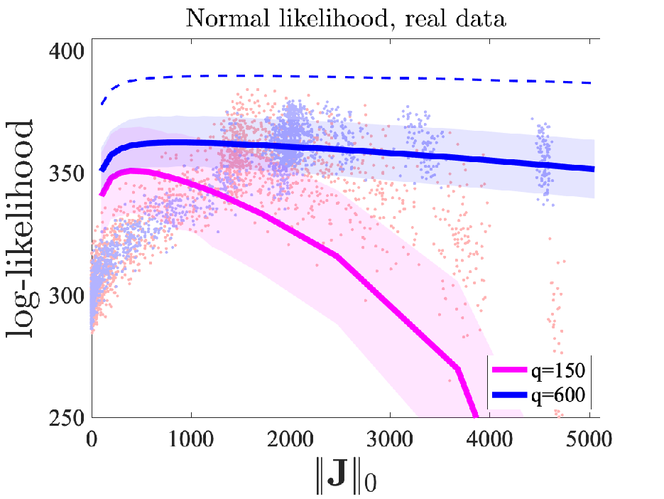
I first investigate the real data using the normal modeling instead of the Student-t. In Fig.2 I report the log-likelihoods for real data obtained from normal models (Eq.2) with IFN constructed using the Pearson estimate of the correlation matrix. The result for the Student-t is reported in this figure with the slashed line for comparison. We observe an overall behavior very similar to what reported for the Student-t approach (see Fig.1), however the values of the log-likelihoods are significantly lower. This indicates that real data from financial log-returns are better modeled with Student-t multivariate probability distributions. This is not a surprise since the literature abundantly reports the inadequacy of normal modeling for financial returns, yet this result is very clean and has a referential value.

I then repeated the experiments on synthetic data generated from multivariate normal and Student-t distributions. Results for normally distributed data are reported in Fig.3. Unsurprisingly, I observe that normal modeling with Pearson estimate of the covariance gives largest likelihoods on normal data. I also observe that the Student-t model with expectation maximization give good results similar to the normal models with Kendal estimate of the covariance. For the t model with expectation maximization optimization I obtain very small differences when the Pearson’s or Kendall’s estimates are used. Indeed the slashed and dotted lines appear overlapping, they are however not coinciding and the Pearson’s estimate give marginally better results.

Results for Student-t distributed data are reported in Fig4. Here, coherently, I observe that Student-t models largely outperform normal models. I also observe that contrary to the normal data case, here the Kendal’s estimates of the covariances is advantageous.

In all the cases I have studied Glasso is outperformed by IFN-LoGo sparse models up to a certain level of sparsity and then they become equivalent.

References

Aste et al. (2010) Tomaso Aste, W Shaw, and Tiziana Di Matteo. Correlation structure and dynamics in volatile markets. New Journal of Physics, 12(8):085009, 2010.
Barfuss et al. (2016) Wolfram Barfuss, Guido Previde Massara, Tiziana Di Matteo, and Tomaso Aste. Parsimonious modeling with information filtering networks. Physical Review E, 94(6):062306, 2016.
Bishop (2006) Christopher M Bishop. Pattern recognition and machine learning. springer, 2006.
Chandra et al. (1936) Mahalanobis Prasanta Chandra et al. On the generalised distance in statistics. In Proceedings of the National Institute of Sciences of India, volume 2, pages 49–55, 1936.
Christensen (2018) Alexander P Christensen. Networktoolbox: Methods and measures for brain, cognitive, and psychometric network analysis in r. The R Journal, 10(2):422–439, 2018.
Christensen et al. (2018) Alexander P Christensen, Yoed N Kenett, Tomaso Aste, Paul J Silvia, and Thomas R Kwapil. Network structure of the wisconsin schizotypy scales–short forms: Examining psychometric network filtering approaches. Behavior Research Methods, 50(6):2531–2550, 2018.
Dempster et al. (1977) Arthur P Dempster, Nan M Laird, and Donald B Rubin. Maximum likelihood from incomplete data via the em algorithm. Journal of the Royal Statistical Society: Series B (Methodological), 39(1):1–22, 1977.
Fang (2018) Kai Wang Fang. Symmetric multivariate and related distributions. CRC Press, 2018.
Hsieh et al. (2014) Cho-Jui Hsieh, Mátyás A Sustik, Inderjit S Dhillon, and Pradeep D Ravikumar. Quic: quadratic approximation for sparse inverse covariance estimation. Journal of Machine Learning Research, 15(1):2911–2947, 2014.
Kotz and Nadarajah (2004) Samuel Kotz and Saralees Nadarajah. Multivariate t-distributions and their applications. Cambridge University Press, 2004.
Lauritzen (1996) Steffen L. Lauritzen. Graphical Models. Oxford:Clarendon, 1996.
Massara and Aste (2018) Guido Previde Massara and Tomaso Aste. Learning clique forests. JMC, To be submitted, 2018.
Massara et al. (2017) Guido Previde Massara, T. Di Matteo, and Tomaso Aste. Network filtering for big data: Triangulated maximally filtered graph. Journal of Complex Networks, 5(2):161, 2017. doi: 10.1093/comnet/cnw015. URL + http://dx.doi.org/10.1093/comnet/cnw015.
Musmeci et al. (2015) N Musmeci, T Aste, and T Di Matteo. Relation between financial market structure and the real economy: Comparison between clustering methods. PLoS ONE, 10(3):e0116201, 2015.
Musmeci et al. (2014) Nicoló Musmeci, Tomaso Aste, and Tiziana Di Matteo. Risk diversification: a study of persistence with a filtered correlation-network approach. arXiv preprint arXiv:1410.5621, 2014.
Pozzi et al. (2013) Francesco Pozzi, Tiziana Di Matteo, and Tomaso Aste. Spread of risk across financial markets: better to invest in the peripheries. Scientific reports, 3:1665, 2013.
Procacci and Aste (2019) Pier Francesco Procacci and Tomaso Aste. Forecasting market states. Quantitative Finance, 19(9):1491–1498, 2019.
Song et al. (2008) Won-Min Song, Tomaso Aste, and Tiziana Di Matteo. Correlation-based biological networks. In Complex Systems II, volume 6802, page 680212. International Society for Optics and Photonics, 2008.
Song et al. (2012) Won-Min Song, Tiziana Di Matteo, and Tomaso Aste. Hierarchical information clustering by means of topologically embedded graphs. PloS one, 7(3):e31929, 2012.
Tibshirani (1996) Robert Tibshirani. Regression shrinkage and selection via the lasso. Journal of the Royal Statistical Society, Series B, 58(1):267–288, 1996.
Tikhonov (1943) Andrey Nikolayevich Tikhonov. On the stability of inverse problems. In Dokl. Akad. Nauk SSSR, volume 39, pages 195–198, 1943.
Tumminello et al. (2005) Michele Tumminello, Tomaso Aste, Tiziana Di Matteo, and Rosario N Mantegna. A tool for filtering information in complex systems. Proceedings of the National Academy of Sciences, 102(30):10421–10426, 2005.
Tumminello et al. (2007) Michele Tumminello, T Di Matteo, T Aste, and Rosario Nunzio Mantegna. Correlation based networks of equity returns sampled at different time horizons. The European Physical Journal B-Condensed Matter and Complex Systems, 55(2):209–217, 2007.