Epipolar Transformers

Yihui HeRui YanKaterina FragkiadakiCarnegie Mellon UniversityPittsburgh, PA 15213{he2@alumni,ruiyan@alumni,katef@cs}.cmu.eduShoou-I YuFacebook Reality LabsPittsburgh, PA 15213shoou-i.yu@fb.com Thanks: Equal contribution

Abstract

A common approach to localize 3D human joints in a synchronized and calibrated multi-view setup consists of two-steps: (1) apply a 2D detector separately on each view to localize joints in 2D, and (2) perform robust triangulation on 2D detections from each view to acquire the 3D joint locations. However, in step 1, the 2D detector is limited to solving challenging cases which could potentially be better resolved in 3D, such as occlusions and oblique viewing angles, purely in 2D without leveraging any 3D information. Therefore, we propose the differentiable “epipolar transformer”, which enables the 2D detector to leverage 3D-aware features to improve 2D pose estimation. The intuition is: given a 2D location $p$ in the current view, we would like to first find its corresponding point $p^{\prime}$ in a neighboring view, and then combine the features at $p^{\prime}$ with the features at $p$ , thus leading to a 3D-aware feature at $p$ . Inspired by stereo matching, the epipolar transformer leverages epipolar constraints and feature matching to approximate the features at $p^{\prime}$ . Experiments on InterHand and Human3.6M ionescu2013human3 show that our approach has consistent improvements over the baselines. Specifically, in the condition where no external data is used, our Human3.6M model trained with ResNet-50 backbone and image size 256 $\times$ 256 outperforms state-of-the-art by 4.23mm and achieves MPJPE 26.9 mm. Code is available¹¹ 1 github.com/yihui-he/epipolar-transformers.

1 Introduction

Refer to caption — Figure 1: Overview of the proposed epipolar transformer, which enables 2D detectors to leverage 3D-aware features for more accurate pose estimation. For a query vector (*e.g*., with length 256) on the intermediate deep feature maps of the reference view (H $\times$ W $\times$ 256), we extract K samples along the corresponding epipolar line in the source view. Dot-product and softmax are used to compute similarity between the query and sampled vectors, which in turn is used to compute the corresponding feature. The corresponding feature is then fused with the reference view feature to arrive at a 3D-aware feature for the reference view.

In order to estimate the 3D pose of a human body or hand, there are two common settings. The first setting is single-view 3D pose estimation zimmermann2017learning; zhang2019end; boukhayma20193d; ge20193d, where the algorithm directly estimates 3D pose from a single image. This is extremely challenging due to the ambiguity in depth when only one view is available. The second setting, which is the focus of our paper, is multi-view 3D pose estimation, where the algorithm can leverage multiple synchronized and geometrically calibrated views to resolve depth ambiguity. A common framework simon2017hand; jafarian2018monet to resolve depth ambiguity and accurately estimate the 3D position of joints follows a two-step process: (1) apply a 2D pose detector on each view separately to localize joints in 2D, and (2) perform robust triangulation based on camera calibration and 2D detections from each view to acquire the 3D position of joints. Robust triangulation is required as the prediction of the 2D pose detector could be incorrect or missing due to occlusions. One main disadvantage of this framework is that the detection in step 1 predicts keypoint positions independently from all other views. Thus, challenging cases that could potentially be better resolved in 3D, such as occlusions and viewing the scene from oblique angles, are all resolved by the detector in 2D without utilizing any 3D information. This could lead to inaccurate detections that are inconsistent in 3D, or the network might require more capacity and training data to resolve these challenging cases.

To this end, we propose the fully differentiable “epipolar transformer” module, which enables a 2D detector to gain access to 3D information in the intermediate layers of the 2D detector itself, and not only during the final robust triangulation phase. The epipolar transformer augments the intermediate features of a 2D detector for a given view (reference view) with features from neighboring views (source view), thus making the intermediate features 3D-aware as shown in Figure 1. To compute the 3D-aware intermediate feature at location $p$ in the reference view, we first find the point corresponding to $p$ in the source view: $p^{\prime}$ , and then fuse the feature at $p^{\prime}$ with the feature at $p$ to get a 3D-aware feature. However, we do not know where the correct $p^{\prime}$ is, so in order to approximate the feature at $p^{\prime}$ , we first leverage the epipolar line generated by $p$ in the source view to limit the potential locations of $p^{\prime}$ . Then, we compute the similarity between the feature at $p$ and the features sampled along the epipolar line. Finally, we perform a weighted sum over the features along the epipolar line as an approximation of the feature at $p^{\prime}$ . The weights used for the weighted sum are the feature similarity. In order to fuse the features at $p$ and $p^{\prime}$ , we propose multiple methods inspired by non-local networks wang2018non. Note that the aforementioned operation is done densely for all locations in an intermediate feature map, so the final output of our module is a set of 3D-aware intermediate features that have the same dimensions as the input feature map.

Since the epipolar transformer is fully differentiable and outputs features with the same dimensions as the input, it can be flexibly inserted into desired locations of a 2D pose detection network and trained end-to-end. The inputs to our network are geometrically calibrated and synchronized multi-view images, and the output of the network is 2D joint locations, which can then further be triangulated to compute 3D joint locations. Note that even though our network outputs 2D joint locations, our network has access to both 2D and 3D features, thus empowering it to leverage more information to achieve more accurate 2D predictions.

To evaluate the performance of our epipolar transformer, we have conducted experiments on Human3.6M ionescu2013human3 and InterHand. On Human3.6M ionescu2013human3, we achieve 26.9 mm mean per-joint position error when using the ResNet-50 backbone on input images of resolution 256 $\times$ 256 and trained without external data. This outperforms the state-of-the-art, Qiu et al. qiu2019cross from ICCV’19 by 4.23 mm. InterHand is an internal multi-view hand dataset where we also consistently outperform the baselines.

In sum, the strengths of our method are as follows.

1.

The epipolar transformer can easily be added into existing network architectures given it is fully differentiable and the output feature dimensions are the same as the input.
2.

The epipolar transformer contains minimal learnable parameters (parameter size is $C$ -by- $C$ , where $C$ is input feature channel size).
3.

The epipolar transformer is interpretable because one can analyze the feature similarity along the epipolar line to gauge whether the matching is successful.
4.

The network learned with the epipolar transformer could generalize to new multi-camera setups that are not included in the training data as long as if the intrinsics and extrinsics are provided.

2 Related Work

Multi-view 3D Human Pose Estimation:

There are many methods proposed for multi-view human pose estimation. Pavllo et al. pavllo20193d proposed estimating 3D human pose in video via dilated temporal convolutions over 2D keypoints. Rhodin et al. rhodin2018learning proposed to leverage multi-view constraints as weak supervision to enhance a monocular 3D human pose detector when labeled data is limited. Our method is most similar to Qiu et al. qiu2019cross and Iskakov et al. iskakov2019learnable, thus we provide a more detailed comparison in the following paragraphs.

Qiu et al. qiu2019cross proposed to fuse features from other views through learning a fixed attention weight for all pairs of pixels for each pair of views. The advantage of this method is that camera calibration is no longer required. However, the disadvantages are (1) more data from each view is needed to train this attention weight, (2) there are significantly more weights to learn when the number of views and the image resolution increases, and (3) during test time, if the multi-camera setup changes, then the attention learned during training time is no longer applicable. On the other hand, although the proposed epipolar transformer relies on camera calibration, it only adds minimal learnable parameters. This makes it significantly easier to train, and thus has less demand on the number of training images per view (Table 4). Furthermore, the network trained with the epipolar transformer can be applied to an unseen multi-camera setup without additional training as long as if the calibration parameters are provided.

Iskakov et al. iskakov2019learnable proposed to learn 3D pose directly via differentiable triangulation hartley2003multiple. One key difference between their learnable triangulation and ours is that Iskakov et al. iskakov2019learnable fuses features with 3D voxel feature maps, which is more computationally expensive and memory intensive than our method that fuses 3D-aware features in 2D feature maps (Table 3).

Multi-view Hand Pose Estimation:

Most 3D hand pose estimation works focus on either monocular RGB images or monocular depth images yuan2017bighand2; yuan2018rgb; xiang2019monocular; dibra2018monocular; zhang2019end; iqbal2018hand; wu2018handmap; zhou2018hbe; ge2018point; cai2018weakly; li2019point; yang2019disentangling; ye2018occlusion. In contrast, there are fewer works on multi-view 3D hand pose estimation, especially two-hand pose estimation due to the difficulty of obtaining multi-view hand data annotations. Simon et al. simon2017hand proposed to iteratively boost single image 2D hand keypoint detection performance using multi-view bootstrapping. Garcia et al. garcia2018first introduced a first-person two-hand action dataset with RGB-D and 3D hand pose annotations. Unfortunately, only the right hand is annotated. To showcase our epipolar transformer on the application of multi-view two-hand pose estimation, we use our internal InterHand dataset.

Epipolar Geometry in Deep Neural Networks:

Prasad et al. prasad2018epipolar applied epipolar constraints to depth regression with the essential matrix. Yang et al. yang2019learning proposed to use symmetric epipolar distance for data-adaptive interest points. MONET jafarian2018monet used epipolar divergence for multi-view semi-supervised keypoint detection. Different from the above methods, we leverage the epipolar geometry for deep feature fusion.

Attention Mechanism:

Vaswani et al. vaswani2017attention first proposed a transformer for sequence modeling based solely on attention mechanisms. Non-local networks wang2018non were introduced for capturing long-term dependencies in videos for video classification. Our approach is named epipolar attention, because we compute attention weights along the epipolar line based on feature similarity and use these weights to fuse features.

3 The Epipolar Transformer

Our epipolar transformer consists of two main components: the epipolar sampler and the feature fusion module. Given a point $p$ in the reference view, the epipolar sampler will sample features along the corresponding epipolar line in the source view. The feature fusion module will then take (1) all the features at the sampled locations in the source view and (2) the feature at $p$ in the reference view to produce a final 3D-aware feature. Note that this is done densely for all locations of an intermediate feature map from the reference view. We now provide the details to the two components.

3.1 The Epipolar Sampler

We first define the notations used to describe the epipolar sampler. Given two images captured at the same time but from different views, namely, reference view $\mathcal{I}$ and source view $\mathcal{I}^{\prime}$ , we denote their projection matrices as $M,\,M^{\prime}\in\mathbb{R}^{3\times 4}$ and camera centers as $C,\,C^{\prime}\in\mathbb{R}^{4}$ in homogeneous coordinates. As illustrated in Figure 1, assuming the camera centers do not overlap, the epipolar line $l$ corresponding to a given query pixel $p=(x,y,1)$ in $\mathcal{I}$ can be deterministically located on $\mathcal{I}^{\prime}$ as follows hartley2003multiple.

\displaystyle l=[M^{\prime}C]_{\times}M^{\prime}M^{+}p,

(1)

where $M^{+}$ is the pseudo-inverse of $M$ , and $[\cdot]_{\times}$ represents the skew symmetric matrix. $p$ ’s corresponding point in the source view: $p^{\prime}$ , should lie on the epipolar line: $l^{T}p^{\prime}=0$ .

Given the epipolar line $l$ of the source view, the epipolar sampler uniformly samples $K$ locations (64 in our experiments) along the visible portion of the epipolar line, i.e., the intersection of $\mathcal{I}^{\prime}$ and $l$ . The sampled locations form a set $\mathcal{P}^{\prime}$ with cardinality $K$ . The epipolar sampler samples sub-pixel locations (real value coordinates) via bilinear interpolation. For query points whose epipolar lines do not intersect with $\mathcal{I}^{\prime}$ at all, we simply skip them. Please also see supplementary materials for details on how to handle image transformations for the epipolar transformer.

3.2 Feature Fusion Module

Ideally, if we knew the ground-truth $p^{\prime}$ in the source view that corresponds to $p$ in the reference view, then all we need to do is sample the feature at $p^{\prime}$ in the source view: $F_{\textrm{src}}(p^{\prime})$ , and then combine it with the feature at $p$ in the reference view: $F_{\textrm{ref}}(p)$ . However, we do not know the ground-truth $p^{\prime}$ . Therefore, inspired by Transformer vaswani2017attention and non-local networks wang2018non, we approximate $F_{\textrm{src}}(p^{\prime})$ by a weighted sum of all the features along the epipolar line as follows:

\displaystyle\overline{F}_{\textrm{src}}(p)=\sum_{p^{\prime}\in\mathcal{P}^{\prime}}\text{sim}(p,p^{\prime})F_{\textrm{src}}(p^{\prime})

(2)

where the pairwise function $\text{sim}(\cdot,\cdot)$ computes the similarity score between two vectors. More specifically, it is the dot-product followed by a softmax function.

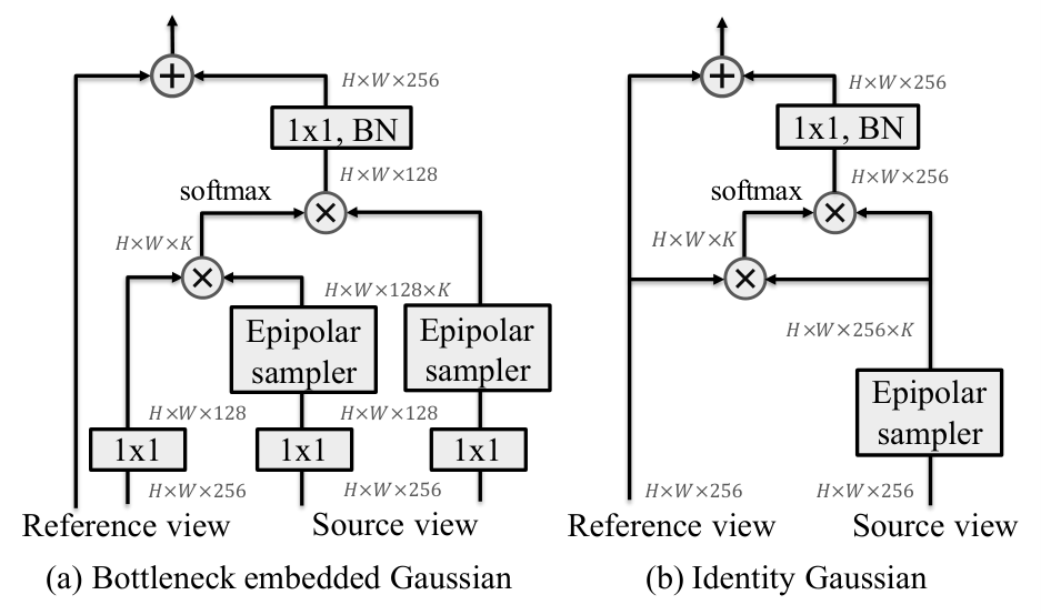
Once we have the feature from the source view: $\overline{F}_{\textrm{src}}(p)$ , we now need to fuse it with the feature in the reference view: $F_{\textrm{ref}}(p)$ . One straightforward way to fuse the features is motivated by the residual block resnet, where the feature from the source view goes through a transformation $W_{z}$ before being added to the features of the reference view as shown in Figure 2 (b) and the following equation:

\displaystyle F_{\textrm{fused}}(p)=F_{\textrm{ref}}(p)+W_{z}(\overline{F}_{\textrm{src}}(p))

(3)

The weights $W_{z}$ are $1\times 1$ convolutions in our experiments. We refer to this method as the Identity Gaussian architecture. Note that the output $F_{\textrm{fused}}$ is of the same shape as the input $F_{\textrm{ref}}$ , thus this property enables us to insert the epipolar transformer module into different stages of many existing networks.

We also explore the Bottleneck Embedded Gaussian architecture, which was popularized by non-local networks wang2018non, as the feature fusion module as shown in Figure 2 (a). Before the epipolar transformer, the features from the reference view and source view goes through an embedded Gaussian kernel, where the channel size is down-sampled by a factor of two, and the output is up-sampled back, so that the shape of the fused feature still matches the input’s shape.

4 Experiments

We have conducted our experiments on two large-scale pose estimation datasets with multi-view images and ground-truth 3D pose annotations: an internal hand dataset InterHand, and a publicly available human pose dataset Human3.6M ionescu2013human3.

InterHand dataset:

InterHand is an internal hand dataset that is captured in a synchronized multi-view studio with 34 color cameras and 46 monochrome cameras. Only the color cameras were used in our experiments. We captured 23 subjects doing various one and two handed poses. We then annotated the 3D location of the hand for 7.6K unique timestamps, which led to 257K annotated 2D hands when we projected the 3D annotations to all 34 2D views. 248K images were used for training, and 9K images were used for testing. For each hand, 21 keypoints were annotated, so there are 42 unique points for two hands.

Human3.6M ionescu2013human3:

Human3.6M ionescu2013human3 is one of the largest 3D human pose benchmarks captured with four cameras and has 3.6M 3D annotations available. The cameras are located at the corners of a rectangular room and therefore have larger baselines. This leads to a major difference compared to InterHand – the viewing angle difference between the cameras in Human3.6M ionescu2013human3 are significantly larger.

Evaluation metric:

During training, we use Mean Squared Error (MSE) between the predicted and ground truth heatmaps as the loss. A ground truth heatmap is generated by applying a 2D Gaussian centered on a joint. To estimate the accuracy of 3D pose prediction, we adopt the MPJPE (Mean Per Joint Position Error) metric. It is one of the most popular evaluation metrics, which is referred to as Protocol $\#1$ in martinez2017simple. It is calculated by the average of the L2 distance between the ground-truth and predictions of each joint.

4.1 Ablation study on InterHand Dataset

We have performed a series of ablation studies on the InterHand dataset to better understand the epipolar transformer, and at the same time to understand the effect of different design choices.

We trained a single-stage Hourglass network newell2016stacked with the epipolar transformer included. To predict the 3D joint positions, we run the 2D detector trained with the epipolar transformer on all the views, and then perform triangulation with RANSAC to get the final 3D joint locations. During prediction time, our 2D detector requires features from the source view, which is randomly selected from the pool of cameras that were used as the source view during training. We downsampled the images to resolution 512 $\times$ 336 for training and testing. Figure 3 visualizes some predictions from our model.

Feature fusion module design:

First, we compare the Bottleneck Embedded Gaussian ((Figure 2 (a)) popularized in the non-local networks wang2018non with Identity Gaussian (Figure 2 (b)). As shown in Table 3, Identity Gaussian performs slightly better. We hypothesize that, unlike video classification wang2018non, pose estimation needs accurate correspondences, so down-sampling in Bottleneck Embedded Gaussian could be detrimental to the performance.

Max or softmax?

We use softmax to obtain the weights along the epipolar line. Another option is to use max because our goal is to find a single “correct” point on the epipolar line. Shown in Table 3, max performs slightly worse than softmax. We hypothesize that it is because softmax produces gradients for all samples on the epipolar line, which helps training.

Architecture design MPJPE (mm) InterHand H3.6M Bottleneck Embedded Gaussian 4.99 35.7 Identity Gaussian + max 4.97 - Identity Gaussian + softmax 4.91 33.1 Table 1: Architecture design comparison for both InterHand and Human3.6M ionescu2013human3. Stage MPJPE (mm) early + late 5.03 early 4.96 late 4.91 Table 2: Epipolar transformer plugged into different stages of Hourglass networks newell2016stacked on InterHand dataset. Inference MPJPE (mm) baseline 5.46 single source view 4.91 multi source views 4.83 Table 3: Different number of neighboring source views for inference on InterHand.

Viewing angle:

We now study how the viewing angle difference of the selected neighboring camera affects the performance of the epipolar transformer. The intuition is that, if the source view has a viewing angle very similar to the reference view, the features from the two views may be too similar, thus not very informative for our fusion module. However, if the views are too far apart, the feature matching becomes harder. There is also a higher chance that a point is occluded in one of the views, which makes matching even harder. Therefore, we experiment with four viewing angle settings during training: 6^∘, 12^∘, 24^∘ and 42^∘. The source view is randomly selected from ten cameras whose viewing angles are closest to the chosen viewing angle. Figure 4 shows examples of the source views with different viewing angles from an example reference view. As also shown in Figure 4, the epipolar transformer is most effective around viewing angle difference 24^∘, which is the setting we use by default for other InterHand experiments.

Which stage to insert the epipolar transformer:

We perform experiments to test the ideal location for inserting the epipolar transformer into a network. We tested two settings: “late” means the epipolar transformer is inserted before the final prediction layer, and “early” means we insert the module before the Hourglass unit newell2016stacked. The exact locations are detailed in the supplementary materials. As shown in Table 3, there is no significant difference where we add the epipolar transformer. In the rest of this paper, we fuse at the late stage by default.

Effect of the number of views used during test time:

We explore how the number of views used during test time affects the final performance. Since there are many different combinations to sample reference and source views, we randomly sample views multiple times (up to 100 times when there are few cameras) and ensure that for each camera there is at least one neighboring camera with viewing angle difference near 24^∘. The baseline compared is a vanilla Hourglass network without using the epipolar transformer. As shown in Figure 5, the network trained with the epipolar transformer consistently outperforms the baseline. When very few views are used (e.g., two views), the relative improvement using the epipolar transformer is around 15%. This supports our argument: epipolar transformers enable the network to obtain better 2D keypoints using information from neighboring views, and the information is crucial when there are fewer views. Even with more views, the epipolar transformer is still able to improve upon the baseline by around 10%.

Figure 5: MPJPE by varying the number of views used for prediction on InterHand. The black lines indicate the standard deviation.

Inference with multiple source views:

The epipolar transformer we introduced is not limited to fusing features from two views. During testing, we can choose different neighboring views as the source view and select the prediction with the highest confidence (i.e., highest peak on the heatmap). As shown in Table 3, we run prediction with ten different neighboring views and select the prediction with the highest confidence for each individual joint. Testing with multi-views reduces the MPJPE error only by 0.1 mm, which is insignificant. The performance might be further improved when training with more than two views, like in MVSNet yao2018mvsnet.

Comparison with cross-view fusion qiu2019cross:

Qiu et al. qiu2019cross learns fixed global attention weights for each pair of views. A limitation of this method is it requires more images per view to learn the attention weights. On InterHand, cross-view fusion qiu2019cross performs even worse than the baseline detector as shown in Table 4. One likely reason is because there are only about 3K images per view on InterHand, instead of 312K images per view on Human3.6M ionescu2013human3. Besides, Human3.6M ionescu2013human3 only has four views, which makes it easier to learn the pairwise attention weights, but learning the weights for 34 views for InterHand is significantly harder.

MPJPE (mm)

InterHand

7k imgs/view

Human3.6M

312k imgs/view

cross-view fusion qiu2019cross

6.29

45.47

baseline

5.46

48.73

epipolar transformer

4.91

33.1

Table 4: Comparison with cross-view fusion qiu2019cross. The baseline is using Hourglass networks newell2016stacked for InterHand and Resnet-50 resnet for Human3.6M ionescu2013human3 without view fusion.

4.2 Human3.6M Dataset

We conducted experiments on the publicly available Human3.6M ionescu2013human3 dataset. We adopt the same training and testing sets as in qiu2019cross, where subjects 1, 5, 6, 7, 8 are used for training, and 9, 11 are for testing.

As there are only four views in Human3.6M ionescu2013human3, we choose a closest view as the source view. We adopt ResNet-50 with image resolution 256 $\times$ 256 proposed in simple baselines for human pose estimation xiao2018simple as our backbone network. We use the ImageNet imagenet pre-trained model pytorch for initialization. The networks are trained for 20 epochs with batch size 16 and Adam optimizer kingma2014adam. Learning rate decays were set at 10 and 15 epochs. Unless specified, we follow Qiu et al. qiu2019cross’s setting and do not do additional data augmentation for a fair comparison. We also follow Qiu et al. qiu2019cross for other hyper-parameters. Following qiu2019cross, as there are only four cameras in this dataset, direct linear transformation (DLT) is used for triangulation (Hartley & Zisserman hartley2003multiple, p.312), instead of RANSAC.

2D Pose Estimation:

Again following Qiu et al. qiu2019cross, the 2D pose estimation accuracy is measured by Joint Detection Rate (JDR), which measures the percentage of the successfully detected joints. A joint is detected if the distance between the estimated location and the ground truth is smaller than half of the head size andriluka20142d.

2D pose estimation results are shown in Table 5. As shown in Qiu et al. qiu2019cross, one way to compute a cross-view score for a specific reference view location is to do a sum or max of the heatmap prediction scores along its corresponding epipolar line in the source view, but this does not lead to good performance. So cross-view fusion qiu2019cross improved performance by fusing with learned global attention. In contrast, the epipolar transformer neither operates on heatmap prediction scores nor does a global fusion. It attends to the intermediate features locally along the epipolar line. Using the same backbone ResNet-50 with input image size 256 $\times$ 256, the model with epipolar transformer achieves 97.01% JDR, which outperforms 95.9% JDR from Qiu et al. qiu2019cross by 1%. The improvement suggests that fusing along the epipolar line is better than fusing globally. We further apply data augmentation which consists of random scales drawn from a truncated normal distribution $\text{TN}(1,0.25^{2},0.75,1.25)$ and random rotations from $\text{TN}(0^{\circ},(30^{\circ})^{2},-60^{\circ},60^{\circ})$ xiao2018simple. JDR is further improved to 98.25% JDR.

	Net	scale	shlder	elb	wri	hip	knee	ankle	root	belly	neck	nose	head	Avg
-	R152	320	88.50	88.94	85.72	90.37	94.04	90.11	-	-	-	-	-	-
sum over epipolar lineqiu2019cross	R152	320	91.36	91.23	89.63	96.19	94.14	90.38	-	-	-	-	-	-
max over epipolar lineqiu2019cross	R152	320	92.67	92.45	91.57	97.69	95.01	91.88	-	-	-	-	-	-
cross-view fusion qiu2019cross	R152	320	95.58	95.83	95.01	99.36	97.96	94.75	-	-	-	-	-	-
cross-view fusion qiu2019cross^⋆	R50	320	95.6	95.0	93.7	96.6	95.5	92.8	96.7	96.4	96.5	96.4	96.2	95.9
cross-view fusion qiu2019cross^⋆	R50	256	86.1	86.5	82.4	96.7	91.5	79.0	100.0	94.1	93.7	95.4	95.5	95.1
epipolar transformer	R50	256	96.44	94.16	92.16	98.95	97.26	96.62	99.89	99.86	99.68	99.78	99.63	97.01
epipolar transformer⁺	R50	256	97.71	97.34	94.85	99.77	98.32	97.55	99.99	99.99	99.76	99.74	99.54	98.25

Table 5: 2D pose estimation accuracy comparison on Human3.6M ionescu2013human3 where no external training data is used unless specified. The metric is joint detection rate, JDR (%).

+

: indicates using data augmentation. "-": We cite numbers from qiu2019cross and these entries were absent.

\star

: We trained the models using released code qiu2019cross. R50 and R152 are ResNet-50 and ResNet-152 resnet respectively. Scale is the input resolution of the network.

Visualization of feature-matching:

The main advantage of the epipolar transformer is that it is easily interpretable through visualizing the feature-matching similarity score along the epipolar line. We visualize the results of feature-matching along the epipolar line for color features, deep features learned without the epipolar transformer, and the features learned through the epipolar transformer. For the color features, we first convert the RGB image to the LAB color space. Then we discard the L-channel and only use the AB channel to be more invariant to light intensity. Figure 6 shows a challenging example where the joint-of-interest is totally occluded in both views. However, given that the features learned with the epipolar transformer have access to multi-view information in the 2D detector itself, the matching along the epipolar line finds the “semantically correct” position, i.e., still finds the occluded right wrist, which is the desired behavior for a pose detector. However, the features without the awareness of the multi-view information have the highest matching score at the “physically correct” location, which is still correct in terms of finding correspondences, but not as useful to reason about occlusions for occluded joints. More examples are shown in the supplementary material.

Effect of the number of views used during test time:

As shown in Figure 7, compared with cross-view qiu2019cross, the models with epipolar transformer still have better performance when there are fewer views. This shows that the epipolar transformer efficiently fuses features from other views.

Figure 7: MPJPE by varying the number of views on Human3.6M ionescu2013human3.

Comparison with state-of-the-art, no external datasets setting:

Table 6 shows the performance of several state-of-the-art methods when no external datasets are used. Our epipolar transformer outperforms the state-of-the-art by a large margin. Specifically, when using triangulation for estimating 3D human poses, epipolar transformer achieves 33.1 mm, which is $\sim$ 12 mm better than cross-view qiu2019cross while using the same backbone network (ResNet-50) and input size (256 $\times$ 256). Using the recursive pictorial structural model (RPSM qiu2019cross) for estimating 3D poses, our epipolar transformer achieves 26.9 mm, which is $\sim$ 14 mm better than the cross-view qiu2019cross equivalent. Furthermore, adding epipolar transformer on ResNet-50 input size 256 $\times$ 256 even surpasses the state-of-the-art result from cross-view qiu2019cross on ResNet-152 input size 320 $\times$ 320 by $\sim$ 4 mm, which is a 13% relative improvement. Our model with data augmentation achieves MPJPE 30.4 mm with triangulation, which is better than the state-of-the-art without even requiring RPSM. We believe one source of improvement comes from the fact that the epipolar transformer finds correspondences and fuses features dynamically based on feature similarity. This is more accurate than cross-view qiu2019cross, which uses a static attention map for all input images from a pair of views.

MPJPE (mm)	Dir	Disc	Eat	Greet	Phone	Photo	Pose	Purch	Sit	SitD	Smoke	Wait	WalkD	Walk	WalkT	Avg
Multi-View Martinez tome2018rethinking	46.5	48.6	54.0	51.5	67.5	70.7	48.5	49.1	69.8	79.4	57.8	53.1	56.7	42.2	45.4	57.0
Pavlakos et al. pavlakos2017harvesting	41.2	49.2	42.8	43.4	55.6	46.9	40.3	63.7	97.6	119.0	52.1	42.7	51.9	41.8	39.4	56.9
Tome et al. tome2018rethinking	43.3	49.6	42.0	48.8	51.1	64.3	40.3	43.3	66.0	95.2	50.2	52.2	51.1	43.9	45.3	52.8
Kadkhodamohammadi & Padoy kadkhodamohammadi2018generalizable	39.4	46.9	41.0	42.7	53.6	54.8	41.4	50.0	59.9	78.8	49.8	46.2	51.1	40.5	41.0	49.1
R50 256 $\times$ 256+triangulate	38.9	46.1	36.2	59.7	46.4	44.7	44.9	37.7	51.2	72.0	48.2	61.0	46.2	45.7	52.0	48.7
R50 256 $\times$ 256+crossview+triangulateqiu2019cross	-	-	-	-	-	-	-	-	-	-	-	-	-	-	-	45.5
R50 256 $\times$ 256+ours+triangulate	30.6	33.2	26.7	28.2	32.8	38.4	29.3	28.9	36.6	45.2	34.3	31.7	33.1	34.8	31.2	33.1
R50 256 $\times$ 256+ours+triangulate ⁺	29.0	30.6	27.4	26.4	31.0	31.8	26.4	28.7	34.2	42.6	32.4	29.3	27.0	29.3	25.9	30.4
R50 256 $\times$ 256+crossview+RPSM qiu2019cross	-	-	-	-	-	-	-	-	-	-	-	-	-	-	-	41.2
R50 256 $\times$ 256+ours+RPSM	25.7	27.7	23.7	24.8	26.9	31.4	24.9	26.5	28.8	31.7	28.2	26.4	23.6	28.3	23.5	26.9
R152 320 $\times$ 320+crossview+triangulateqiu2019cross	34.8	35.8	32.7	33.5	34.4	38.2	29.7	60.7	53.1	35.2	41.0	41.6	31.9	31.4	34.6	38.3
R152 320 $\times$ 320+crossview+RPSM	28.9	32.5	26.6	28.1	28.3	29.3	28.0	36.8	42.0	30.5	35.6	30.0	29.3	30.0	30.5	31.2

Table 6: Comparison with state-of-the-art methods on Human3.6M ionescu2013human3, where no additional training data is used unless specified. The metric is MPJPE (mm). "⁺": rotation and scaling augmentation. "-": models trained using released code qiu2019cross, where the per action MPJPE evaluation were not provided.

Comparison with state-of-the-art, with external datasets setting:

Table 3 shows the performance of several state-of-the-art methods when external datasets are used. Iskakov et al. iskakov2019learnable established a 22.8 mm MPJPE RANSAC baseline with extra data from MS-COCO coco and MPII andriluka20142d. They further proposed the learnable weighted triangulation (algebraic w/ conf) and volumetric triangulation NIPS2018_7755; moon2018v2v; Tung_2019_CVPR, which achieve 19.2 mm and 17.7 mm respectively. We fine-tune a MS-COCO+MPII pre-trained ResNet-152 384 $\times$ 384 released in iskakov2019learnable on Human3.6M ionescu2013human3 and achieve 19.0 mm, which is the best among methods using vanilla triangulation. Besides, the epipolar transformer contributes very little to the number of parameters and computation.

	complexity		pre-train		fine-tune		err.
	param	MAC	COCO	MPII	H36M	MPII
crossview+tri.	560M	212B			✓		38.3
crossview+RPSM	560M	212B			✓		31.2
crossview+tri.	560M	212B			✓	✓	27.9
crossview+RPSM	560M	212B			✓	✓	26.2
triangulate	69M	204B	✓	✓	✓	✓	22.8
algebraic	80M	210B	✓	✓	✓	✓	24.5
algebraic w/ conf	80M	210B	✓	✓	✓	✓	19.2
volumetric⁺	81M	360B	✓	✓	✓	✓	17.7
ours+tri.	69M	204B	✓	✓	✓		19.0

Table 7: Comparison with state-of-the-art methods using external datasets on Human3.6M ionescu2013human3. +: data augmentation (i.e., cube rotation iskakov2019learnable). "err.": the error metric is MPJPE (mm). "tri." stands for triangulation. Number of Parameters and MAC (multiply-add operations) are calculated using THOP³³ 3 github.com/Lyken17/pytorch-OpCounter.

4.3 Limitations

The biggest limitation of our method is the reliance on precise geometric camera calibration. Poor calibration will lead to inaccurate epipolar lines thus incorrect feature matching. Another limitation of our method is that the viewing angle of neighboring camera views should not be too large, otherwise there is a high likelihood a 3D point might be occluded in one of the views, which will make feature matching more difficult.

5 Conclusion

We proposed the epipolar transformer, which enables 2D pose detectors to leverage 3D-aware features through fusing features along the epipolar lines of neighboring views. Experiments not only show improvement over the baseline on Human3.6M ionescu2013human3 and InterHand, but also demonstrate that our method can improve multi-view pose estimation especially when there are few cameras. Qualitative analysis of feature matching along the epipolar line also show that the epipolar transformer can provide more accurate matches in difficult scenarios with occlusions. Finally, the epipolar transformer has very few learnable parameters and outputs features with the same dimension as the input, thus enabling it to be easily augmented to existing 2D pose estimation networks. For future work, we believe that the epipolar transformer can also benefit 3D vision tasks such as deep multi-view stereo yao2018mvsnet.

References

(1) Mykhaylo Andriluka, Leonid Pishchulin, Peter Gehler, and Bernt Schiele. 2d human pose estimation: New benchmark and state of the art analysis. In Proceedings of the IEEE Conference on Computer Vision and Pattern Recognition, 2014.
(2) Adnane Boukhayma, Rodrigo de Bem, and Philip HS Torr. 3d hand shape and pose from images in the wild. In Proceedings of the IEEE Conference on Computer Vision and Pattern Recognition, 2019.
(3) Yujun Cai, Liuhao Ge, Jianfei Cai, and Junsong Yuan. Weakly-supervised 3d hand pose estimation from monocular rgb images. In Proceedings of the European Conference on Computer Vision, 2018.
(4) Cristian Sminchisescu Catalin Ionescu, Fuxin Li. Latent structured models for human pose estimation. In Proceedings of the IEEE International Conference on Computer Vision, 2011.
(5) Ricson Cheng, Ziyan Wang, and Katerina Fragkiadaki. Geometry-aware recurrent neural networks for active visual recognition. In Advances in Neural Information Processing Systems. 2018.
(6) Jia Deng, Wei Dong, Richard Socher, Li-Jia Li, Kai Li, and Li Fei-Fei. Imagenet: A large-scale hierarchical image database. In Proceedings of the IEEE Conference on Computer Vision and Pattern Recognition, 2009.
(7) Endri Dibra, Silvan Melchior, Ali Balkis, Thomas Wolf, Cengiz Oztireli, and Markus Gross. Monocular rgb hand pose inference from unsupervised refinable nets. In Proceedings of the IEEE Conference on Computer Vision and Pattern Recognition Workshops, 2018.
(8) Guillermo Garcia-Hernando, Shanxin Yuan, Seungryul Baek, and Tae-Kyun Kim. First-person hand action benchmark with rgb-d videos and 3d hand pose annotations. In Proceedings of the IEEE Conference on Computer Vision and Pattern Recognition, 2018.
(9) Liuhao Ge, Zhou Ren, Yuncheng Li, Zehao Xue, Yingying Wang, Jianfei Cai, and Junsong Yuan. 3d hand shape and pose estimation from a single rgb image. In Proceedings of the IEEE Conference on Computer Vision and Pattern Recognition, 2019.
(10) Liuhao Ge, Zhou Ren, and Junsong Yuan. Point-to-point regression pointnet for 3d hand pose estimation. In Proceedings of the European Conference on Computer Vision, 2018.
(11) Richard Hartley and Andrew Zisserman. Multiple view geometry in computer vision. Cambridge university press, 2003.
(12) Kaiming He, Xiangyu Zhang, Shaoqing Ren, and Jian Sun. Deep residual learning for image recognition. In Proceedings of the IEEE Conference on Computer Vision and Pattern Recognition, 2016.
(13) Catalin Ionescu, Dragos Papava, Vlad Olaru, and Cristian Sminchisescu. Human3.6m: Large scale datasets and predictive methods for 3d human sensing in natural environments. IEEE transactions on pattern analysis and machine intelligence, 2013.
(14) Umar Iqbal, Pavlo Molchanov, Thomas Breuel Juergen Gall, and Jan Kautz. Hand pose estimation via latent 2.5d heatmap regression. In Proceedings of the European Conference on Computer Vision, 2018.
(15) Karim Iskakov, Egor Burkov, Victor Lempitsky, and Yury Malkov. Learnable triangulation of human pose. arXiv preprint arXiv:1905.05754, 2019.
(16) Yasamin Jafarian, Yuan Yao, and Hyun Soo Park. Monet: Multiview semi-supervised keypoint via epipolar divergence. arXiv preprint arXiv:1806.00104, 2018.
(17) Abdolrahim Kadkhodamohammadi and Nicolas Padoy. A generalizable approach for multi-view 3d human pose regression. arXiv preprint arXiv:1804.10462, 2018.
(18) Diederik P Kingma and Jimmy Ba. Adam: A method for stochastic optimization. arXiv preprint arXiv:1412.6980, 2014.
(19) Shile Li and Dongheui Lee. Point-to-pose voting based hand pose estimation using residual permutation equivariant layer. In Proceedings of the IEEE Conference on Computer Vision and Pattern Recognition, 2019.
(20) Tsung-Yi Lin, Michael Maire, Serge Belongie, James Hays, Pietro Perona, Deva Ramanan, Piotr Dollár, and C Lawrence Zitnick. Microsoft coco: Common objects in context. In Proceedings of the European Conference on Computer Vision, 2014.
(21) Julieta Martinez, Rayat Hossain, Javier Romero, and James J Little. A simple yet effective baseline for 3d human pose estimation. In Proceedings of the IEEE International Conference on Computer Vision, 2017.
(22) Gyeongsik Moon, Ju Yong Chang, and Kyoung Mu Lee. V2v-posenet: Voxel-to-voxel prediction network for accurate 3d hand and human pose estimation from a single depth map. In Proceedings of the IEEE Conference on Computer Vision and Pattern Recognition, 2018.
(23) Alejandro Newell, Kaiyu Yang, and Jia Deng. Stacked hourglass networks for human pose estimation. In Proceedings of the European Conference on Computer Vision, 2016.
(24) Adam Paszke, Sam Gross, Soumith Chintala, and Gregory Chanan. Pytorch, 2017.
(25) Georgios Pavlakos, Xiaowei Zhou, Konstantinos G Derpanis, and Kostas Daniilidis. Harvesting multiple views for marker-less 3d human pose annotations. In Proceedings of the IEEE Conference on Computer Vision and Pattern Recognition, 2017.
(26) Dario Pavllo, Christoph Feichtenhofer, David Grangier, and Michael Auli. 3d human pose estimation in video with temporal convolutions and semi-supervised training. In Proceedings of the IEEE Conference on Computer Vision and Pattern Recognition, 2019.
(27) Vignesh Prasad, Dipanjan Das, and Brojeshwar Bhowmick. Epipolar geometry based learning of multi-view depth and ego-motion from monocular sequences. arXiv preprint arXiv:1812.11922, 2018.
(28) Haibo Qiu, Chunyu Wang, Jingdong Wang, Naiyan Wang, and Wenjun Zeng. Cross view fusion for 3d human pose estimation. In Proceedings of the IEEE International Conference on Computer Vision, 2019.
(29) Helge Rhodin, Jörg Spörri, Isinsu Katircioglu, Victor Constantin, Frédéric Meyer, Erich Müller, Mathieu Salzmann, and Pascal Fua. Learning monocular 3d human pose estimation from multi-view images. In Proceedings of the IEEE Conference on Computer Vision and Pattern Recognition, 2018.
(30) Tomas Simon, Hanbyul Joo, Iain Matthews, and Yaser Sheikh. Hand keypoint detection in single images using multiview bootstrapping. In Proceedings of the IEEE Conference on Computer Vision and Pattern Recognition, 2017.
(31) Denis Tome, Matteo Toso, Lourdes Agapito, and Chris Russell. Rethinking pose in 3d: Multi-stage refinement and recovery for markerless motion capture. In 2018 International Conference on 3D Vision (3DV), 2018.
(32) Hsiao-Yu Fish Tung, Ricson Cheng, and Katerina Fragkiadaki. Learning spatial common sense with geometry-aware recurrent networks. In The IEEE Conference on Computer Vision and Pattern Recognition, 2019.
(33) Ashish Vaswani, Noam Shazeer, Niki Parmar, Jakob Uszkoreit, Llion Jones, Aidan N Gomez, Łukasz Kaiser, and Illia Polosukhin. Attention is all you need. In Advances in neural information processing systems, 2017.
(34) Xiaolong Wang, Ross Girshick, Abhinav Gupta, and Kaiming He. Non-local neural networks. In Proceedings of the IEEE Conference on Computer Vision and Pattern Recognition, 2018.
(35) Xiaokun Wu, Daniel Finnegan, Eamonn O’Neill, and Yong-Liang Yang. Handmap: robust hand pose estimation via intermediate dense guidance map supervision. In Proceedings of the European Conference on Computer Vision, 2018.
(36) Donglai Xiang, Hanbyul Joo, and Yaser Sheikh. Monocular total capture: Posing face, body, and hands in the wild. In Proceedings of the IEEE Conference on Computer Vision and Pattern Recognition, 2019.
(37) Bin Xiao, Haiping Wu, and Yichen Wei. Simple baselines for human pose estimation and tracking. In Proceedings of the European Conference on Computer Vision, 2018.
(38) Guandao Yang, Tomasz Malisiewicz, Serge Belongie, Erez Farhan, Sungsoo Ha, Yuewei Lin, Xiaojing Huang, Hanfei Yan, and Wei Xu. Learning data-adaptive interest points through epipolar adaptation. In Proceedings of the IEEE Conference on Computer Vision and Pattern Recognition Workshops, 2019.
(39) Linlin Yang and Angela Yao. Disentangling latent hands for image synthesis and pose estimation. In Proceedings of the IEEE Conference on Computer Vision and Pattern Recognition, 2019.
(40) Yao Yao, Zixin Luo, Shiwei Li, Tian Fang, and Long Quan. Mvsnet: Depth inference for unstructured multi-view stereo. In Proceedings of the European Conference on Computer Vision, 2018.
(41) Qi Ye and Tae-Kyun Kim. Occlusion-aware hand pose estimation using hierarchical mixture density network. In Proceedings of the European Conference on Computer Vision, 2018.
(42) Shanxin Yuan, Bjorn Stenger, and Tae-Kyun Kim. Rgb-based 3d hand pose estimation via privileged learning with depth images. arXiv preprint arXiv:1811.07376, 2018.
(43) Shanxin Yuan, Qi Ye, Bjorn Stenger, Siddhant Jain, and Tae-Kyun Kim. Bighand2. 2m benchmark: Hand pose dataset and state of the art analysis. In Proceedings of the IEEE Conference on Computer Vision and Pattern Recognition, 2017.
(44) Xiong Zhang, Qiang Li, Hong Mo, Wenbo Zhang, and Wen Zheng. End-to-end hand mesh recovery from a monocular rgb image. In Proceedings of the IEEE International Conference on Computer Vision, 2019.
(45) Yidan Zhou, Jian Lu, Kuo Du, Xiangbo Lin, Yi Sun, and Xiaohong Ma. Hbe: Hand branch ensemble network for real-time 3d hand pose estimation. In Proceedings of the European Conference on Computer Vision, 2018.
(46) Christian Zimmermann and Thomas Brox. Learning to estimate 3d hand pose from single rgb images. In Proceedings of the IEEE International Conference on Computer Vision, 2017.

Supplementary Materials: Epipolar Transformer for Multi-view Pose Estimation

Appendix A Dealing with Image Transformations

As the epipolar transformer relies on camera calibration, any spatial transformation applied on the image needs to be reflected in the calibration parameters.

Data augmentation:

Data augmentation like rotation, scaling and cropping can still be performed with the epipolar transformer. The projection matrix needs to be updated accordingly when the image is transformed with an affine transformation parameterized by $A\in\mathbb{R}^{2\times 2}$ and $b\in\mathbb{R}^{2}$ :

\displaystyle M:=\begin{bmatrix}A&b\\ \mathbf{0}^{T}&1\\ \end{bmatrix}M

(4)

Different scaling and cropping parameters can be applied separately to the reference view and source view.

Scaling of projection matrices:

We should pay special attention to scale the projection matrices for resizing or pooling images.

Suppose the input image is spatially down-sampled $s_{x}$ and $s_{y}$ times along the x-axis and y-axis, the projection matrix is updated as follows:

\displaystyle M:=\begin{bmatrix}1/s_{x}&0&(1-s_{x})/2s_{x}\\ 0&1/s_{y}&(1-s_{y})/2s_{y}\\ 0&0&1\\ \end{bmatrix}M

(5)

The coordinates are aligned with the center of pixels rather than the top-left corners, which is important for extracting features at precise locations in the epipolar transformer.

Appendix B 2D Prediction Visualization in Video

In skeletons $\_$ 1min.mp4, we visualize 2D predicted skeletons on Human3.6M ionescu2013human3 testing set. All methods are with ResNet-50 resnet and image size 256 $\times$ 256, corresponding to the following three entries in Table 6 respecitively:

1.

R50 256 $\times$ 256 + triangulate
2.

R50 256 $\times$ 256 + crossviewqiu2019cross + triangulate
3.

R50 256 $\times$ 256 + ours + triangulate

In twohand $\_$ 30.mp4, we visualize 2D predicted hands on InterHand testing set. The video consists of the visualizations of the ground truth, the 5.46 mm baseline and 4.91 mm model with epipolar transformer in Table 3.

Appendix C Stages to Add Epipolar Transformer

In our experiments, we compared the performance between adding epipolar transformer in the early stage and adding in the late stage (see Table 3, paragraph Which stage to insert the epipolar transformer). Figure 8 illustrates the precise places of inserting the epipolar transformer for the “early” and “late” settings in an one-stage Hourglass network newell2016stacked on InterHand and ResNet-50 resnet simple baseline xiao2018simple on Human3.6M ionescu2013human3 respectively.

Appendix D Epipolar Transformer Visualization on Human3.6M ionescu2013human3

We show the visualizations of feature matching similarity for images from Human3.6M ionescu2013human3 in Figure 9, Figure 10, and Figure 11. In Figure 9, we show a visualization of the matching results of an easy case in Human3.6M ionescu2013human3. Note that in this case, our prediction aligns well with the ground truth. Using the features from the baseline, that is, deep features extracted without using the epipolar transformer, the matched point denoted by the yellow dot is also accurate. However, for more difficult cases in Figure 10 and Figure 11, the deep features learned with the epipolar transformer can perform more accurate matching.

Appendix E Epipolar Transformer Visualization on InterHand

We show visualization of feature matching similarity for images from InterHand. As shown in Figure 12, the color features have multiple peaks in similarity due to the different fingers having similar colors. On the other hand, for most cases deep features trained through the epipolar transformer are able to discriminate the correct finger from all the other similar looking fingers.