Coherent States and Generalized Hermite Polynomials for Fractional statistics - interpolating from fermions to bosons

In an earlier paperSatish1, we analyzed the Hilbert space derived from the “commutator”

in the case where $\theta=\frac{2\pi M}{N}$ where $M,N$ are co-prime non-zero natural numbers and where we also define $z=e^{i\theta}$. This algebra was inspired by the properties of anyons and was intended to interpolate between fermionic and bosonic statistics. In particular, we had considered the general case where the vacuum state had a non-zero eigenvalue. When the vacuum state has a zero eigenvalue, however, we are naturally led to the study of variables $\xi$, such that $\xi^{N}=0$. Such variables, which may be referred to as generalized Grassmann variables have been the subject of much study in the past Biedenharn; MacFarlane; Chaichian, of which the most complete and relevant is Chaichian. The difference is that since our focus is on the full range of fractional statistics between fermions and bosons in 2+1 dimensions, we study a full calculus starting with integration rules to a physically reasonable construction of the path integral for the free energy.

In addition to the generalization of the Grassmann variables mentioned above, there is also a rather simple geometrical picture that emerges from the arithmetic for the operators in the algebra Hallnas. Akin to the fuzzy solid representations used for the angular momentum algebra, we prove that the relevant geometrical picture here is a pancake that goes from a sphere (for $N=2$) to a plane (for $N\rightarrow\infty$).

We are going to, in this paper, analyze several properties of the Hilbert space, in the special and physically interesting case where the vacuum state has zero eigenvalue for the operators $\beta\alpha$, as well as $\alpha^{\dagger}\alpha$. Hence, in the notation of Satish1, we set $\lambda_{0}=0$.

For general integer $N$, we deduce the following properties.

1. 1.

   States are labeled by their eigenvalues under $\beta\alpha$, i.e.,

   	$\displaystyle\beta\alpha\ket{\lambda_m}=\lambda_{m}\ket{\lambda_m}$
   	$\displaystyle Eigenvalues:\>\lambda_{0}\equiv\lambda_{N}=0,\lambda_{1}=1,\lambda_{2}=1+z,\lambda_{3}=1+z+z^{2},\>...\>,$
   	$\displaystyle\lambda_{N-1}=1+z+z^{2}+...+z^{N-2},\>and\>\>\lambda_{N}=1+z+z^{2}+...+z^{N-1}=0$
   	$\displaystyle Eigenstates:\>\ket{\lambda_0}\equiv\ket{0},\ket{\lambda_1},\ket{\lambda_2},...\ket{\lambda_{N-1}},\>\>\>\>\>\>\>\>$
   	$\displaystyle\ket{\lambda_{N}}\equiv\ket{\lambda_0}\equiv\ket{0}\>\>\>\>\>\>\>\>$
   	$\displaystyle\innerproduct{\lambda_m}{\lambda_n}=\delta_{nm}\>\>\>\>\>\>\>\>\>\>\>\>$		(2)

   The eigenvectors can be constructed to be orthogonal, since these are also the eigenvectors of the usual number operator $\alpha^{\dagger}\alpha$.

   We propose to call these states “overons”, since they represent one of the two ways to flip anyons (“over” and “under”). The complex conjugate states would be then called “underons”. In Appendix 1, we study possible dynamical system analogs that might result from such excitations.

2. 2.

   The actions of the operators are

   	$\displaystyle\alpha\ket{0}\equiv\alpha\ket{\lambda_{N}}\equiv\alpha\ket{\lambda_0}=0$
   	$\displaystyle\alpha\ket{\lambda_m}=\sqrt{\lambda_{m}}\ket{\lambda_{m-1}}\>\>\>\>\>\>m>0$
   	$\displaystyle\beta\ket{\lambda_{m-1}}=\sqrt{\lambda_{m}}\ket{\lambda_m}$		(3)

3. 3.

   A consistent identification is $\beta=\alpha^{T},\>\alpha=\beta^{T}$, i.e., the commutator is $\alpha\alpha^{T}-z\alpha^{T}\alpha=1$..

4. 4.

   When we take the complex conjugate of the basic commutator, we get, by an entirely similar procedure to the above, that the eigenstates of $a^{\dagger}a^{*}$ are $\ket{\lambda_m^*}$. The chain of reasoning is

   	$\displaystyle\alpha\alpha^{T}-z\alpha^{T}\alpha=1$
   	$\displaystyle\alpha^{*}\alpha^{\dagger}-z^{-1}\alpha^{\dagger}\alpha^{*}=1$
   	$\displaystyle(\alpha^{T}\alpha)\ket{\lambda_m}=\lambda_{m}\ket{\lambda_m}$
   	$\displaystyle\alpha^{\dagger}\alpha^{*}\ket{\lambda^*_m}=\lambda_{m}^{*}\ket{\lambda_m^*}$		(4)

   Taking the complex conjugate of the third equation above, we get $\left(\ket{\lambda_m}\right)^{*}=\ket{\lambda_m^*}$. This leads to the equations

   	$\displaystyle\alpha\ket{\lambda_m}=\sqrt{\lambda_{m}}\ket{\lambda_{m-1}}$
   	$\displaystyle\alpha^{*}\ket{\lambda_m^*}=\sqrt{\lambda_{m}^{*}}\ket{\lambda_{m-1}^*}$		(5)

   Continuing, we can now write $\ket{\lambda_m^*}$ as a linear combination of the $\ket{\lambda_m}$. In fact, it is easy to see, from the geometry of the eigenvectors on the complex plane in Fig. 3, that

   $\displaystyle\ket{\lambda_m^*}=z^{-(m-1)}\ket{\lambda_m}$

   (6)

   Using this,

   	$\displaystyle\alpha\ket{\lambda_m^*}=z^{-(m-1)}\sqrt{\lambda_{m}}\ket{\lambda_m}=\sqrt{\lambda_{m}}\ket{\lambda_m^*}\>\>\>\>\>\>\>\>\>\>\>\>\>\>$
   	$\displaystyle\alpha^{\dagger}\ket{\lambda_m}=(\alpha^{T})^{*}\ket{\lambda_m}=\left(\alpha^{T}\ket{\lambda_m^*}\right)^{*}=\left(z^{-(m-1)}\alpha^{T}\ket{\lambda_m}\right)^{*}=z^{m-1}\sqrt{\lambda_{m+1}^{*}}\ket{\lambda_{m+1}^*}$
   	$\displaystyle=z^{-1}\sqrt{\lambda_{m+1}^{*}}\ket{\lambda_{m+1}}\>\>\>\>\>\>\>\>\>\>\>\>\>\>\>\>\>\>\>\>\>\>\>\>\>\>\>\>\>$		(7)

   Using this, and defining $\bra{\lambda_m}$ as the usual hermitian conjugate transpose of $\ket{\lambda_m}$,

   	$\displaystyle\alpha\alpha^{\dagger}\ket{\lambda_m}=|\lambda_{m+1}|\ket{\lambda_m}\>\>\>\>\>\>\>$
   	$\displaystyle\alpha^{\dagger}\alpha\ket{\lambda_m}=|\lambda_{m}|\ket{\lambda_m}$
   	$\displaystyle\rightarrow\>\>\bra{\lambda_m}\alpha\alpha^{\dagger}-\alpha^{\dagger}\alpha\ket{\lambda_m}=|\lambda_{m+1}|-|\lambda_{m}|$		(8)

   The traditional “number” operator $\alpha^{\dagger}\alpha$ is diagonal in the same basis that $\alpha^{T}\alpha$ is. Since $\alpha^{\dagger}\alpha$ is a hermitian operator, it is consistent that the $\ket{\lambda_m}$ is an orthonormal basis Banks.

5. 5.

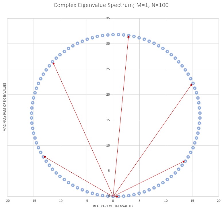
   The eigenvalue spectrum of $\beta\alpha\equiv\alpha^{T}\alpha$ (magnitude as well as complex vectors) is as below and in reference Satish1 and is plotted in Fig. 1. Note that we have $\theta=\frac{2\pi M}{N}$ and we have used $M=1$ for the graphs in Fig. 1.

   	$\displaystyle\lambda_{0}=0\>\>\>\>\>\>\>\>\>\>\>\>\>\>\>\>\>\>\>\>\>\>\>\>\>\>\>\>$
   	$\displaystyle\lambda_{m}=z^{0}+z^{1}+...+z^{m-1}=\frac{1-e^{im\theta}}{1-e^{i\theta}}=e^{i\frac{(m-1)\theta}{2}}\frac{\sin{\frac{m\theta}{2}}}{\sin{\frac{\theta}{2}}}$		(9)

   

   

6. 6.

   The matrices $\alpha$ and $\beta=\alpha^{T}$ are displayed explicitly below, for $\theta=\frac{2\pi M}{N}$. They are $N\times N$ matrices, since the eigenstates are $N$-dimensional vectors. The eigenvectors are as below

   $\displaystyle\ket{\lambda_0}=\left(\begin{array}[]{c}{\bf 1}\\ 0\\ 0\\ 0\\ .\\ .\\ .\\ 0\\ 0\end{array}\right)\>\>\>,\>\>\ket{\lambda_1}=\left(\begin{array}[]{c}0\\ {\bf 1}\\ 0\\ 0\\ .\\ .\\ .\\ 0\\ 0\end{array}\right)\>\>\>,\>\>\ket{\lambda_2}=\left(\begin{array}[]{c}0\\ 0\\ {\bf 1}\\ 0\\ .\\ .\\ .\\ 0\\ 0\end{array}\right)\>\>\>...\>\>\ket{\lambda_{N-1}}=\left(\begin{array}[]{c}0\\ 0\\ 0\\ 0\\ .\\ .\\ .\\ 0\\ {\bf 1}\end{array}\right)\>\>\>\>\>\>\>\>\>\>\>\>\>\>\>\>\>\>\>\>\>\>\>\>\>\>\>\>\>\>$

   while the operators are

   	$\displaystyle\alpha=\left(\begin{array}[]{cccccccc}{\bf 0}&\>\>\>1&\>\>\>0&\>\>\>0&\>\>\>0&...&\>\>\>0&0\\ 0&\>\>\>{\bf 0}&\>\>\>\sqrt{1+z}&\>\>\>0&\>\>\>0&...&\>\>\>0&0\\ 0&\>\>\>0&\>\>\>{\bf 0}&\>\>\>\sqrt{1+z+z^{2}}&\>\>\>0&...&\>\>\>0&0\\ 0&\>\>\>0&\>\>\>0&\>\>\>{\bf 0}&\>\>\>\sqrt{1+z+z^{2}+z^{3}}&...&\>\>\>0&0\\ .\\ .\\ .\\ 0&\>\>\>0&\>\>\>0&\>\>\>0&\>\>\>0&...&\>\>\>{\bf 0}&\sqrt{1+z+z^{2}+...+z^{N-1}}\\ 0&\>\>\>0&\>\>\>0&\>\>\>0&\>\>\>0&...&\>\>\>0&{\bf 0}\end{array}\right)$
   	$\displaystyle\beta=\alpha^{T}=\left(\begin{array}[]{cccccccc}{\bf 0}&\>\>\>0&\>\>\>0&\>\>\>0&\>\>\>0&...&\>\>\>0&0\\ 1&\>\>\>{\bf 0}&\>\>\>0&\>\>\>0&\>\>\>0&...&\>\>\>0&0\\ 0&\>\>\>\sqrt{1+z}&\>\>\>{\bf 0}&\>\>\>0&\>\>\>0&...&\>\>\>0&0\\ 0&\>\>\>0&\>\>\>\sqrt{1+z+z^{2}}&\>\>\>{\bf 0}&\>\>\>0&...&\>\>\>0&0\\ 0&\>\>\>0&\>\>\>0&\>\>\>\sqrt{1+z+z^{2}+z^{3}}&\>\>\>{\bf 0}&...&\>\>\>0&0\\ .\\ .\\ .\\ 0&\>\>\>0&\>\>\>0&\>\>\>0&\>\>\>0&...&\sqrt{1+z+z^{2}+...+z^{N-1}}&{\bf 0}\end{array}\right)$

   while the commutator is

   	$\displaystyle\alpha\alpha^{T}-\alpha^{T}\alpha=\alpha\beta-\beta\alpha=\left(\begin{array}[]{cccccccc}{\bf 1}&\>\>\>0&\>\>\>0&\>\>\>0&\>\>\>0&...&0\\ 0&\>\>\>{\bf z}&\>\>\>0&\>\>\>0&\>\>\>0&...&\>\>\>0&0\\ 0&\>\>\>0&\>\>\>{\bf z^{2}}&\>\>\>0&\>\>\>0&...&\>\>\>0&0\\ 0&\>\>\>0&\>\>\>0&\>\>\>{\bf z^{3}}&\>\>\>0&...&\>\>\>0&0\\ 0&\>\>\>0&\>\>\>0&\>\>\>0&\>\>\>{\bf z^{4}}&...&\>\>\>0&0\\ .\\ .\\ .\\ 0&\>\>\>0&\>\>\>0&\>\>\>0&\>\>\>0&...&{\bf z^{N-2}}&\>\>\>0\\ 0&\>\>\>0&\>\>\>0&\>\>\>0&\>\>\>0&...&\>\>\>0&{\bf z^{N-1}}\end{array}\right)\>\>\>\>\>\>\>\>\>\>\>\>$
   	$\displaystyle=diag\left[1,z,z^{2},z^{3},...,z^{N-1}\right]\>\>\>\>\>\>\>\>\>\>\>\>\>\>\>\>\>\>\>\>\>\>\>\>\>\>\>\>\>\>\>\>\>\>\>\>\>\>\>\>\>\>\>\>\>\>\>\>\>\>\>\>\>\>\>\>\>\>\>\>\>\>\>\>\>\>\>\>\>\>\>\>$		(78)

   and

   	$\displaystyle\alpha\alpha^{\dagger}-\alpha^{\dagger}\alpha=diag\left[1-0,|\lambda_{2}|-|\lambda_{1}|,|\lambda_{3}|-|\lambda_{2}|,...,|\lambda_{N}|-|\lambda_{N-1}|\right]$
   	$\displaystyle=diag[1,\frac{\sin\frac{2\theta}{2}-\sin\frac{\theta}{2}}{\sin\frac{\theta}{2}},\frac{\sin\frac{3\theta}{2}-\sin\frac{2\theta}{2}}{\sin\frac{\theta}{2}},\frac{\sin\frac{4\theta}{2}-\sin\frac{3\theta}{2}}{\sin\frac{\theta}{2}},...,\frac{-\sin\frac{(N-1)\theta}{2}}{\sin\frac{\theta}{2}}]\>\>\>\>\>\>\>\>\>\>\>\>\>\>\>\>\>\>$		(79)

   and

   	$\displaystyle\alpha\alpha^{\dagger}-{\mathcal{C}}\alpha^{\dagger}\alpha=1$
   	$\displaystyle{\mathcal{C}}=diag[\frac{|\lambda_{1}|-1}{|\lambda_{0}|},\frac{|\lambda_{2}|-1}{|\lambda_{1}|},\frac{|\lambda_{3}|-1}{|\lambda_{2}|},...,\frac{|\lambda_{N}|-1}{|\lambda_{N-1}|}]$		(80)

   The top-left component $\frac{|\lambda_{1}|-1}{|\lambda_{0}|}$ of $\mathcal{C}$ is not determined by the above commutator since $\alpha^{\dagger}\alpha=0$ for the state $\ket{\lambda_0}$. However, we can determine it by taking the limit of the expressions for $\lambda_{0}\rightarrow 0$ as in Satish1; it becomes $\cos\theta$, which is $-1$ for the fermion limit and $+1$ for the bosonic limit. Hence $\mathcal{C}$ is $-\cal I$ (the identity matrix) for fermions and $+\cal I$ for bosons.

7. 7.

   When we compute scattering amplitude matrix elements for different particles, we will have to re-order the annihilation and creation operators, then will be left with a product of terms like $\alpha^{m}\beta^{m}$, i.e.,

   	$\displaystyle\alpha\beta=(1+z\>\beta\alpha)$
   	$\displaystyle\alpha^{2}\beta^{2}=(1+z)+(z+2z+z^{3})\beta\alpha+z^{4}\beta^{2}\alpha^{2}\>$
   	$\displaystyle...$

   When we compute expectation values in the vacuum state (i.e., $\bra{0}\alpha^{m}\beta^{m}\ket{0}$), only the constant terms will be left and they are, for the first few powers

   	$\displaystyle m=1\>\>\>\rightarrow\>\>\>1$
   	$\displaystyle m=2\>\>\>\rightarrow\>\>\>1+z$
   	$\displaystyle m=3\>\>\>\rightarrow\>\>\>1+2z+2z^{2}+z^{3}$
   	$\displaystyle m=4\>\>\>\rightarrow\>\>\>1+3z+5z^{2}+6z^{3}+5z^{4}+3z^{5}+z^{6}$
   	$\displaystyle m=5\>\>\>\rightarrow\>\>\>1+4z+9z^{2}+15z^{3}+20z^{4}+22z^{5}+20z^{6}+15z^{7}+9z^{8}+4z^{9}+z^{10}$
   	$\displaystyle m=6\>\>\>\rightarrow(1,5,14,29,49,71,90,101,101,90,71,49,29,14,5,1)\>\>\>\>\>\>\>\>\>\>\>\>\>\>\>$		(81)

   where we have represented the polynomial by just its coefficients (the Mahonian numbers Mahon) in the last case. As can be checked quickly, these are the polynomials $\lambda_{1},\lambda_{2}\times\lambda_{1},\lambda_{3}\times\lambda_{2}\times\lambda_{1}$ etc.

The most general geometrical construction is

and observe that

we obtain the equation

This equation can be re-phrased as an invariant of the group that underlies the algebra. The algebra can be written most simply with the creation/annihilation operators as

In Equation (17), the two limits $\theta\rightarrow 0$ and $\theta\rightarrow\pi$ are consistent on both sides of the equation. Additionally, ${\cal L}$ and ${\cal M}$ are the matrices as defined in Equation (23) and $S_{D}$ is the real, diagonal matrix

which is the finite-difference Laplacian of a diagonal matrix with absolute values of the eigenvalues along the diagonal. In this notation, from Equation (17), $Z=D_{m}(|\lambda|)$, so that the commutator in that equation can be written in the interesting form

Incidentally, for $N=3$, this is consistent with the previous paper’sSatish1 Equation (25) at the points resolved within the fuzzy ellipsoid ($Z=J_{z}=0,\pm\frac{1}{2}$). In this case,

satisfies both the Equations (25) and following in the previous paper Satish1, i.e.,

We have already noted the equivalence for $N=2$.

The surface described by the above equation is pancake-shaped aligned along the z-axes, as in Fig. 2.

For large $N$, we can write the solutions to the above equation (in terms of the polar radius coordinate $\rho$) as

which yields concentric circular strips on the plane $z=\frac{1}{2}$, where each state has radius $\propto\sqrt{m+\frac{1}{2}}$. This is the usual picture for Landau levels; here this is a geometrical representation of the usual bosonic levels.

To show how a spherical object for $N=2$ transforms into the flat plane in the $N\rightarrow\infty$ limit, we can compute the surface area of the pancake. The area integral is computed (define $a=\sin\frac{\theta}{4}$) as

Clearly, this diverges as $a\rightarrow 0$, which corresponds to $N\rightarrow\infty$, since $\theta=\frac{2\pi}{N}$.

We plot the area as a function of $a$ in Fig. 3. Indeed, the pancake like closed surface turns into the infinite plane as $N\rightarrow\infty$.

For a general $N$-type algebra, we can write down an eigenstate for $\alpha$ as

The above expansion is identical to the usual formula for boson coherent states in the limit $N\rightarrow\infty$, as well as for fermion coherent states at $N=2$ (the usual Grassmann variables). We also define the “bra” vector as the adjoint vector, where $\xi^{\dagger}$ is the adjoint of $\xi$ and is independent of $\xi$, i.e.,

That they are eigenvectors may be checked by applying $\alpha$ to the state and using Equation (3), we postulate that $\xi$ and $\alpha$ commute. Additionally, we posit that $\xi^{N}=0$ and the transposition relations (the matrix ${\cal C}_{0}$ is as defined in Equation (12))

What sort of object is $\xi$? The two relations above make sense only if $\xi$ were itself an $N\times N$ matrix, for consistency, we assume is a direct product of a “generalized Grassmann matrix” and a unit $N\times N$ matrix in the states’ eigenbasis, hence, commutes with all other complex number matrices in the same eigenbasis. Hence $\xi^{T}$ and $\xi^{\dagger}$ are all reasonable objects to define. The above statements and equations are also consistent with the statement that a term like $\xi^{\dagger}\xi$ is “real”. This is true, since $\cal C$ is a real matrix. In addition, since $\xi\sim\alpha$, it is consistent to require the equations below (in line with Equation (4)),

The description of this algebra is similar to the treatment in reference Chaichian, however, the difference here is that these variables are directly coherent state variables, as in the usual definition Murayama1.

Some auxiliary results are written below. Again, note that all these products are scalars times the unit matrix.

Note that in the $N\rightarrow\infty$ limit, when $z\rightarrow 1$, $\innerproduct{\xi}{\xi}=e^{\xi^{\dagger}\xi}$, which is appropriate for bosonic coherent states. Taking the limit in the opposite direction, the behavior is appropriate for fermions, when $N=2$ the algebra automatically yields $\innerproduct{\xi}{\xi}=e^{\xi^{\dagger}\xi}=e^{-\xi\xi^{\dagger}}$.

We can now write down, from the expansion in Equation (28), a series expansion for $\frac{1}{\innerproduct{\xi}{\xi}}$, which also terminates at the term $(\xi^{\dagger})^{N-1}\xi^{N-1}$, since higher powers are $0$.

The following integrals are postulated, in order to match the boundary cases for bosonic variables as well as for fermionic $(N=2)$ Grassmanns. We set

which is consistent with

While the first (moment) variety of integral can be checked for the limiting fermion and boson cases, the second variety of integrals (without the normalization) cannot be properly defined in the bosonic cases since it isn’t convergent. The first method can be treated as a regularized integral.

The one-variable version of these integrals can be defined, in consistency with the above equations, as

It is possible to define an identity operator, so that (using Equation (29)),

The trace of an operator $A$ that commutes with and can be taken through $\xi$ is

where we have used the regularized integrals from Equation (29).

The action integral is, for a “Hamiltonian” $\frac{\mathcal{H}}{k_{B}T}\equiv\frac{\epsilon}{k_{B}T}\alpha^{\dagger}\alpha={\mathcal{K}}\epsilon\alpha^{\dagger}\alpha$,

The bracketed term can be “split” into sub-integrals using the identity operator from Equation (40). We define $\xi_{N}={\cal C}_{0}^{-1}\xi_{0}$ and $\delta\tau=\frac{{\mathcal{K}}}{N}$.

References

• (1) Ramakrishna, Satish Algebra for Fractional Statistics - interpolating from fermions to bosons arxiv:2005.02172, submitted to Nucl. Phys. B
• (2) Ramakrishna, Satish A generalized q-commutator and other diversions Paper in preparation
• (3) Chaichian, M., Demichev, A. P. Path Integrals with Generalized Grassmann Variables arxiv:9504016
• (4) MacMahon, P.A. Combinatory Analysis, Vol. 1 and 2, Cambridge Univ.Press, Cambridge, 1915, reprinted by Chelsea, New York (1955).
• (5) Fivel, Daniel I. Interpolation between Fermi and Bose Statistics Using Generalized Commutators Phy. Rev. Lett. 65, 3361 (1990)
• (6) Iida, Shinji, Kuratsuji, Hiroshi Quantum Algebra near q=1 and a Deformed Symplectic Structure Phy. Rev. Lett. 69, 1833 (1992)
• (7) Greenberg, Oscar W. Interactions of particles having small violations of statistics Physica A 180, 419-427 (1992)
• (8) Leinaas, J. M., Myrheim, J, Nuovo Cimento B 37 (1977) 1.
• (9) Rao, Sumathi Anyons: a primer, arxiv.org/abs/hep-th/9209066
• (10) Khare, Avinash Fractional Statistics And Quantum Theory, World Scientific, 2n​d​e​d.2^{nd}\>ed. 2005.
• (11) Boschi-Filho, H. , Farina, C. , de Souza Dutra, A. , The Partition Function for an Anyon-Like Oscillator, arxiv.org/abs/hep-th/9410098
• (12) Lorek A., Ruffing A., Wess J., A q-deformation of the Harmonic Oscillator Zeitschrift fur Physik C Particles and Fields, June 1997, Volume 74, Issue 2, pp. 369-377 also arxiv:hep-th/960516v1 22 May 1996
• (13) Sang, Chung Won New q-Deformed Fermionic Oscillator Algebra and Thermodynamics, J. Adv. Physics Vol. 4, pp. 1-4, 2015
• (14) MacFarlane A. J., On q-analogues of the quantum harmonic oscillator and the quantum group S​U​(2)qSU(2)_{q} J. Phys. A.: Math. Gen 22 4581
• (15) Biedenharn L. C., The quantum group SUq(2) and a q-analogue of the boson operators J. Phys. A.: Math. Gen 22 L873
• (16) Murayama, H. Unpublished Lecture Notes “Statistical Mechanics of Bosons” http://hitoshi.berkeley.edu/221B/bosons.pdf
• (17) Murayama, H. Unpublished Lecture Notes “Statistical Mechanics of Fermions” http://hitoshi.berkeley.edu/221B/fermions.pdf
• (18) Lavagno A., Narayana Swamy P. Generalized thermodynamics of q-deformed bosons and fermions arxiv:cond-mat/0111112v1 7 Nov 2000
• (19) Banks, T. Quantum Mechanics: An Introduction Taylor & Francis (2018)
• (20) Griffiths, David J. Introduction to Quantum Mechanics Prentics Hall (1994)
• (21) Laughlin R. B., Anomalous Quantum Hall Effect: An incompressible Quantum Fluid with Fractionally Charged Excitations Phys. Rev. Lett. 50, 18 (1983)
• (22) Hallnas, Martin The fuzzy sphere, a noncommutative geometry http://courses.theophys.kth.se/SI2350/fuzzy.pdf
• (23) Oliveira, E. C de, Machado, J. A. T. A Review of Definitions for Fractional Derivatives and Integral Vol. 2014 doi.org/10.1155/2014/238459