Deep convolutional generative adversarial networks for traffic data imputation encoding time series as imagesJournal: Transportation Research Part C: Emerging Technologies
Abstract
Sufficient high-quality traffic data are a crucial component of various Intelligent Transportation System (ITS) applications and research related to congestion prediction, speed prediction, incident detection, and other traffic operation tasks. Nonetheless, missing traffic data are a common issue in sensor data which is inevitable due to several reasons, such as malfunctioning, poor maintenance or calibration, and intermittent communications. Such missing data issues often make data analysis and decision-making complicated and challenging. In this study, we have developed a generative adversarial network (GAN) based traffic sensor data imputation framework (TSDIGAN) to efficiently reconstruct the missing data by generating realistic synthetic data. In recent years, GANs have shown impressive success in image data generation. However, generating traffic data by taking advantage of GAN based modeling is a challenging task, since traffic data have strong time dependency. To address this problem, we propose a novel time-dependent encoding method called the Gramian Angular Summation Field (GASF) that converts the problem of traffic time-series data generation into that of image generation. We have evaluated and tested our proposed model using the benchmark dataset provided by Caltrans Performance Management Systems (PeMS). This study shows that the proposed model can significantly improve the traffic data imputation accuracy in terms of Mean Absolute Error (MAE) and Root Mean Squared Error (RMSE) compared to state-of-the-art models on the benchmark dataset. Further, the model achieves reasonably high accuracy in imputation tasks even under a very high missing data rate ( 50%), which shows the robustness and efficiency of the proposed model.
Keywords:
Traffic data imputation , generative adversarial networks , realistic data generation , time-dependent encoding , deep convolutional neural networks1 Introduction
Dissemination of accurate traffic data is an essential requirement for supporting advanced traffic management system operations. Different types of sensors, such as loop detectors, radar sensors, and video detectors, are installed in freeways and arterials for traffic data collection purposes. The data collected from these sensors can be used to detect traffic congestion or incidents [Chakraborty et al. 2018a, Chakraborty et al. 2018b, Chakraborty et al. 2019], provide travel time information to road users [Lu et al. 2017, Gan et al. 2017], and support decision making at the traffic operation and planning levels [Shi and Abdel-Aty 2015, Ma et al. 2017]. However, missing data are quite common in traffic sensor data due to issues such as malfunctioning, poor maintenance or calibration, and intermittent communications [Lee and Coifman 2011]. According to the California Performance Measurement System (PeMS), only 67% of the sensors in District 7 of southern California (Los Angeles) were found to be working as expected in December 2018 [Armanious 2019]. While data from sensors with a high percentage of missing data can be discarded from further usage, an alternate approach is to impute the missing records, so that these sensors’ data can still be used for subsequent analysis. This is particularly important for traffic-related studies that require traffic records to be complete, such as traffic flow analysis methods. Therefore, it is important to develop an effective traffic data imputation method which can handle missing traffic records even at a high percentage of missing data.
Traditionally, traffic data imputation has been done using prediction or interpolation methods that use historical traffic data or traffic data from adjacent sensors or time points to impute missing records [Nihan 1997, Ghosh et al. 2007, Allison 2001, Chang et al. 2012]. However, these methods often fail to explicitly capture the spatio-temporal variations, which can lead to unreliable performance. Another class of imputation techniques relies on statistical learning models such as Markov chains or principal component analysis to learn the schema of the traffic data matrix [Lv et al. 2014, Ni and Leonard 2005, Qu et al. 2009]. However, these methods require the assumptions on the probability distribution of traffic data, which makes them difficult to apply in real-world scenarios. Also, these methods do not work well when handling large proportions of missing data, which is a common issue in real-world too. With the recent advancements in deep learning techniques and their success in image recognition and imputation tasks, traffic data imputation problem has been tackled using these new techniques that treat the data imputation problem as a corrupted data denoising problem [Duan et al. 2016, Ku et al. 2016, Asadi and Regan 2019]. However, modeling the strong time dependency of the time-series data is one of the major challenges in the application of these imputation techniques. To address this issue, we propose a novel Gramian Angular Summation Field (GASF) encoding method in this study to embed the traffic data for our model input, precisely preserving its time dependency. We then train a deep convolutional generative adversarial network (DCGAN) to generate realistic synthetic data for missing data imputation.
In recent years, deep learning based Generative Adversarial Networks (GANs) have been successful in generating impressively realistic synthetic data by modeling the real data distributions [Goodfellow et al. 2014, Goodfellow et al. 2016]. Further, by taking advantage of convolutional neural networks (CNNs), DCGANs [Radford et al. 2015] have shown remarkable ability in generating high quality synthetic image data for many applications such as image-to-image translation [Isola et al. 2017], audio generation [Donahue et al. 2018], and image super-resolution [Ledig et al. 2017]. Such impressive performance in modeling the original data distribution has made DCGANs a strong candidate for data imputations [Yeh et al. 2017, Lee et al. 2019].
In this study, we have developed a traffic data imputation framework based on generative adversarial network (TSDIGAN) to efficiently resolve the missing data problem. Our proposed model treats the data imputation problem as a synthetic data generation problem. The novel GASF encoding method used in this study helps to embed the strong temporal dependency of the time-series data, thereby translating the time-series imputation problem to an image imputation problem. We evaluate our proposed model using the benchmark PeMS dataset [PeMS 2014] and compare its performance with other baseline statistical and deep learning models. We also investigate the capability of our proposed model for large-scale applications by clustering sensors into homogeneous groups and learning imputation models for each cluster of sensors. Thus, the major contributions of our study are as follows:
- 1.
Our proposed model takes advantage of deep learning based generative models, enabling users to treat the data imputation problem as a data generation problem. Such a generative framework can impute the missing data using the best-fitting generated realistic looking data, such that it is adaptive and robust in imputing the missing records, even at a high percentage of missing data.
- 2.
Our novel traffic time-series data-encoding technique using GASF method preserves the time dependency of traffic data without losing the underlying temporal dependency information. This proposed encoding method helps the model to learn the point-wise temporal relations between time-series traffic data.
- 3.
Our proposed model achieved reasonably high accuracy in imputation task for missing data ratios ranging from 5% to 90%, making it robust and reliable under challenging high missing data percentages. Additionally, training the proposed model using year-long traffic data takes less than 8 minutes, making it efficient and scalable for large-scale implementation. Therefore, we also evaluated our proposed model across extensive sensor groups of California District 5, showing the feasibility for large-scale practical applications. The proposed model has been found to improve the imputation accuracies in terms of Mean Absolute Error (MAE) and Root Mean Squared Error (RMSE) compared to the state-of-the-art benchmark imputation models, while achieving comparable results in terms of Mean Relative Error (MRE).
The rest of this paper is organized as follows. Section 2 provides a brief description of related work regarding traffic missing data imputations, followed by the details of our methodology in Section 3. Section 4 provides a detailed description of the data used in this study, results obtained using our proposed model compared to the baseline models. Finally, Section 5 summarizes the contributions of our study and its implications for future research.
2 Literature Review
Since several ITS applications require high-quality traffic data, a significant amount of studies have been done in the past on missing traffic data imputation. As summarized by Li et al. 2014, traffic data imputation methods can be broadly divided into three categories: prediction methods, interpolation methods, and statistical learning methods. Some recent studies have also applied deep learning-based methods like stacked denoising autoencoders (DSAE) to estimate missing traffic data.
Prediction based models such as the Autoregressive Integrated Moving Average (ARIMA) model [Nihan 1997, Park et al. 1998], support vector regression (SVR) [Castro-Neto et al. 2009], and Bayesian networks (BNs) [Ghosh et al. 2007] use the historical observations to predict the future data points. These prediction-based models assume that the future data points follow the typical trace as the historical data. Prediction based methods can usually estimate data points effectively over the short-term and for samples whose missing data ratio is low. However, their performance drops significantly for long-term imputation problems. Further, these methods only use observations from the history before the missing data points, while any valuable information available after the missing data points is not utilized.
Interpolation based models, another popular method for missing data imputation, include temporal neighboring model or historical model [Yin et al. 2012, Smith et al. 2003, Allison 2001] and k-NN model [Al-Deek et al. 2004]. The basic idea of the historical model is to impute missing data points using the average historical value reported by the same sensor for the same time periods. Therefore, historical models assume that the daily traffic flow has strong consistency. However, they do not use the information of the inherent daily variation to improve the imputation performance. In contrast, the k-NN method utilizes the average historical value for a given day of the week from the same sensor or neighboring sensors to impute missing data, instead of considering the overall average. However, these interpolation-based models often fail to explicitly capture the spatial-temporal variations, which can lead to unreliable imputation results.
Statistical based models such as probabilistic principal component analysis (PPCA) [Qu et al. 2009] and Markov Chain Monte Carlo (MCMC) methods [Ni and Leonard 2005] have been proposed to overcome the limitations mentioned above and improve imputation accuracy based on statistical modeling. These statistical methods assume a probability distribution model for the traffic data and impute the missing data using the observed data with optimized parameters. However, these models do not work well when the proportion of missing data are significantly high, especially for the case when an entire day of traffic data is missing [Anandkumar et al. 2014, Tan et al. 2013], a situation fairly common in real-world scenarios.
In recent years, deep learning based models using denoising stacked autoencoders (DSAE) have been studied to overcome the shortcomings of the traditional data imputation models [Duan et al. 2016, Ku et al. 2016]. Such models have been found to be successful in obtaining reliable performance by converting the data imputation problem into a data cleaning/denoising problem. Typically, DSAE models extract the useful inherent correlations from the original data, recovering them from the high-level features with noise reduction. The basic idea of DSAE models is to train a “recovery tool" using both the raw data and imputed missing data. Therefore, a well-trained model will recover missing data with more reliable estimations compared to the conventional methods described above. However, such feature extraction compresses data into lower dimensions, which limits the variability of the model and makes model outcomes less interpretable.
Besides this, recurrent neural network (RNN) based GAN has also been used for time series data imputation. For instance, conditional Long Short-Term Memory (LSTM) based GAN has been used for medical data generation [Esteban et al. 2017] and traffic data prediction [Lv et al. 2018]. On the other hand, Gated Recurrent Unit (GRU) based GAN has been used for multivariate time series generation [Luo et al. 2018]. Similarly, Asadi and Regan 2019 adopted convolution recurrent autoencoder using bidirectional-LSTM layer as the encoder layer for spatial-temporal missing data imputation. However, training such RNN networks generally take significantly longer time, particularly when handling the long time sequence (200) [Li et al. 2019]. Recently, Chen et al. 2019 proposed parallel data based GAN model, which used the real data and synthetically generated data simultaneously for traffic data imputation to achieve state-of-the-art results. However, using the original daily traffic time series data as the latent space limits the generative ability of GAN based model thereby requiring each sensor to have its own generative model. This leads to training and managing a large number of models thereby making it difficult for large-scale application.
In this study, we propose a traffic data imputation framework based on generative adversarial network (TSDIGAN) encoding the time series into images. This enables us to treat the data imputation problem as image generation problem, thereby utilizing the significant developments in DCGAN based image generation problems. We also compare our proposed model performance with the most recent state-of-the-art traffic data imputation based on GAN, proposed by Chen et al. 2019 to show the efficacy of our proposed model.
3 Methodology
In this section, we provide the step by step details of our proposed TSDIGAN framework. We first explain the notation used in this study and then introduce the Gramian Angular Summation Field (GASF) time-series encoding and the basic concepts of GAN. The details of the proposed TSDIGAN model framework is then discussed, followed by the large-scale implementation technique.
3.1 Notation
We first describe the abstract mathematical expressions used in this study. These notations will be used throughout the paper by default. Let us assume that the traffic flow time-series data for a given sensor on a given day is denoted by , where is the observation of . For 5-minute interval traffic flow data used in this study, is given by . The combined daily time-series data for each sensor can then be represented as , where represents the total number of days involved. Finally, we use a binary corrupted mask as an indicator variable to flag whether the data for is present or missing. This leads to Equation 1.
| (1) |
can be divided into two subsets: (1) fully observed datasets, which do not have missing data points in any samples, denoted as , and (2) corrupted datasets, which contain missing data points in each samples, denoted as . For each sample, we flag whether the data points are missing or not using the corrupted mask which can also be divided into two subset matrices: (for fully observed datasets) and (for corrupted datasets). Next, we describe the first task in our proposed TSDIGAN framework: converting time-series traffic data to GASF encoding, which enables treatment of the time-series imputation problem as an image imputation problem.
3.2 Gramian Angular Summation Field
Encoding time-series data as images have been widely used for time-series classification, audio data recognition, and similar other tasks. One of the popular approaches to tackle this problem is the spectrogram based method. For example, Cummins et al. 2017, Zhao et al. 2018 converted the speech/sound time series data into spectrogram using Short-time Fourier Transform (STFT) for recognition of emotional speech and locate image regions which produce sounds. Also, Lefebvre et al. 2017 estimated traffic flow by converting the spectrum features of the acoustic sensors signal data using Mel Frequency Cepstral Coefficients (MFCCs). However, such spectrogram based methods require careful parameter selection for precise inverse operation, and the imputation task of typical daily traffic volume data is unlikely to benefit from it [Wang and Oates 2015]. Another approach to encode the time series to images is to combine the spatial-temporal information as a 2D matrix. For instance, Zhuang et al. 2018, Kim et al. 2018 merged the ordered road segments/stations and time-series traffic data to form a 2D matrix that can be used by CNN to extract the spatial-temporal information. However, obtaining well-ordered sensor information in a complex, large-scale network is difficult and time-consuming. Further, the model needs to be retrained completely even when a single sensor is added or removed to the network.
To alleviate these issues, in this study, we adopted the Gramian Angular Summation Field (GASF), which has been demonstrated to improve CNN features extraction [Wang and Oates 2015, Wang et al. 2017]. The GASF has the following advantages. First, it helps to preserve and enhance the temporal correlations by considering the trigonometric sum between each time instance point. Second, the character of bijection provides directly and precisely inverse operation without the need for any specific parameter selection.
We rescaled the given preprocessed traffic flow time-series data to such that we can represent the data in polar coordination system. Therefore, for daily traffic time-series data , the volume data and time stamp are encoded as angular cosine and radius () respectively, given by the following equation:
| (2) |
where, is a constant regularization factor.
After transforming the traffic time-series data by using the above equation, the temporal correlation between each point can be identified by the GASF matrix denoted as :
| (3) |
The main diagonal of contains the original angular/value information. As mentioned above, the rescaled time-series data belongs to the set so that the mapping between and its corresponding angular cosine value is bijective. These characteristics allow us to precisely recover (inverse transform) the traffic time-series data from the GASF matrix using the following equation:
| (4) |
Here, we replace the suspect 0 value with 1 to avoid the zero division error and apply log transformation to avoid skewed distribution. Then, we rescale and transform the preprocessed 1-D daily traffic flow data into image-like GASF matrix using Equations 2 and 3. The image-like matrix embedding with temporal dependencies helps convolutional neural networks (CNNs) to effectively extract the required features [LeCun et al. 1998]. We used this image-like GASF matrix as the input of our proposed GAN model. Finally, the daily traffic flow data can be recovered from the GASF matrix using Equation 4.
3.3 Generative Adversarial Networks
Generative adversarial nets (GAN) were introduced as an effective tool for data augmentation and data generation. The basic GAN architecture is shown in Figure 1, which consists of two parts: a generator and a discriminator [Goodfellow et al. 2014]. The generator takes a random vector as input, sampled from a noise distribution , to output a corresponding synthetic data sample . The discriminator takes a real sample from the original dataset and the synthetic sample as inputs to estimate the probability that the generated and real sample comes from the same distribution. In our case, the original dataset and the real sample is given by and respectively, which are obtained from GASF encoding. Both and usually consist of multi-layer perceptions (MLPs).

The discriminator and generator compete with each other like a two-player minimax game, where both the discriminator and the generator are trained simultaneously. During the training, the generator tries to fool the discriminator, while the discriminator tries to distinguish the real samples from the synthetic samples by solving the value function formulated as:
| (5) |
After alternative training of both the discriminator and generator, the distribution of synthetic samples produced by the generator converges with the distribution of the original real data . In other words, the generator produces such realistic synthetic samples that the discriminator can no longer distinguish them from the original data samples.
3.4 TSDIGAN Architecture
In this subsection, we introduce the framework of our proposed model in details. The architecture of our proposed discriminator and generator is shown in Figure 2.

In the discriminator module, we used strided convolution (expressed as “Conv Stride: 2” in Figure 2a). In contrast, for the generator module, we used fractional-strided convolutions (expressed as “Deconv Stride: 2” in Figure 2b). We then applied Batch Normalization (BatchNorm) layers to stabilize the learning process and prevent model collapse. BatchNorm was used for all layers, except the input layer of the discriminator and the output layer of the generator to avoid sample oscillation. We used LeakyReLU as the activation function for all layers to provide non-linearity, except in the output layers of both the discriminator and generator, where we used the sigmoid and tanh functions as the activation functions to produce the scalar and synthetic data respectively. Moreover, the latent random vector was sampled from the normal distribution.
To help the CNN model learn more effectively, we repeated the first and last traffic flow data points at the head and tail of the three times instead of doing the “zero-padding". Therefore, the dimensions of the input traffic data vector transformed to 294 = , with the GASF matrix dimensions being . This same padding value was removed after training. Additionally, we applied a Gaussian filter on the to reduce the inherent noise and improve the quality of the GAN-generated synthetic data [Susmelj et al. 2017]. The initial learning rate was set to 0.0002 along with the Adam optimizer. GANs are however known to suffer from mode collapse issues frequently, when the training model often sticks to only few modes of the true distribution ignoring the other modes [Radford et al. 2015]. To prevent the potential mode collapse in this study, we randomly assigned the training label from 0.8 to 1.1 and 0.0 to 0.3 for positive and negative labels respectively. Also, we randomly flipped 10% of the training labels in each mini-batch [Salimans et al. 2016]. These strategies helped to prevent the discriminator/generator from trapping into state of extremely high confidence and stabilize the training process during our experiments.
3.4.1 Maximum Mean Discrepancy
After training our TSDIGAN model, the generator can generate synthetic daily traffic flow dataset that looks “close" to the real data sampled from the original fully observed dataset . During the training phase, the generator generates the same number of samples as used for training. Therefore, in this case is obviously equal to . In general, a well-trained GAN can implicitly learn the distribution of the original fully observed dataset . Visual inspection of synthetic traffic flow data is one recommended means of determining if a TSDIGAN model is well-trained, which is also considered as the intuitive way to inspect GANs based models [Borji 2019].
In addition, we utilized the maximum mean discrepancy (MMD) method as the quantifiable tool to measure the similarity between the two distributions and [Gretton et al. 2007] using the following equation:
| (6) |
Here, represent the kernel function, and we used the radial basis function (RBF) kernel for MMD score calculation as described in Esteban et al. 2017. We recommend interested readers refer to Esteban et al. 2017 for more details. Figure 3 shows the sample MMD score trace over 60 training epochs. Therefore, training of the proposed TSDIGAN was verified not only through visual inspection of its synthetic traffic flow data, but also by observing stable convergence of the score.

3.5 TSDIGAN Imputation Model
After training our TSDIGAN using the fully observed dataset as described in Section 3.4, we used our trained model for missing traffic data imputation. In this subsection, we introduce the imputation (or inpainting) framework shown in Figure 4. The basic idea of our imputation framework is similar to GAN based image inpainting [Yeh et al. 2017, Yu et al. 2018] in that we searched the most representative from as the input for the generator to use in generating a realistic synthetic data for each specific .

From the basic concept of the GAN, we know that the generator learns the distribution from original fully observed dataset , and generate the synthetic dataset without any missing points from the learned distributions. We could thus use the synthetic data sample to fill in the missing points in via the corrupted mask vector . However, for the given incomplete data vector , which should we use to generate the most reasonable data? The question above can be described as searching for the “closest" from to generate missing values constituting the best “overlay" synthetic traffic flow data , based on the observed part of the given data vector . To accomplish this goal and inspired by Yeh et al. 2017, Luo et al. 2018, we designed the masked reconstruction loss denoted as . For any given , the masked reconstruction loss can be formulated as:
| (7) |
It should be noted that by multiplying the masked missing vector , only the observed part of is used for calculating the masked reconstruction loss, and the represents element-wise multiplication. Thus, the “closest" latent vector can be represented as:
| (8) |
Finally, we used the synthetic traffic flow data generated from the “closest" to fill in the missing part of . We summarize this imputation module step by step as shown in Algorithm 1.
3.6 Large-Scale Implementation
Deep learning models are promising for the traffic data imputation task; however, their practical applications on large-scale statewide level requires further investigation. In this subsection, we investigate the capability of our proposed TSDIGAN model for large-scale real world application. Typically, traffic sensors over extensive wide coverage involves a wide variation of traffic data characteristics. Grouping all the sensors together in a single cluster can make the model training significantly harder due to multiple modes present in the data generated from the distinct variations in traffic data generated across the different sensors. Further, this can lead to model instability and mode collapse, thereby making the training process significantly difficult and lead to poor model performance. On the other hand, training a model individually for each sensor leads to a significantly larger number of models training and maintenance/updates, making it difficult to large-scale application. For example, in the recent state-of-the-art traffic data imputation study by Chen et al. (2019) using parallel data based GAN model, a total of 294 models across the 147 districtwide sensors were developed for weekday and non weekdays. In this study, we chose a middle ground where we group the sensors based on their inherent traffic data characteristics such that models generated for each cluster can be focused towards the cluster-specific traffic variation characteristics. More specifically, we use k-means clustering [MacQueen et al. 1967, Berkhin 2006] to group the sensors based on their daily traffic flow patterns because of it’s simplified approach and computation efficiency.
Let us assume, we have sensors in the traffic sensor networks. As mentioned in Section 3.1, the fully observed data provided by a given sensor is denoted as . Therefore, the traffic flow values for each sensor over a given set of days () can be denoted as a matrix with the dimensions . At each time instance , we extracted the features of this matrix by taking the quantiles value along the , and augmenting them into one long feature vector with the shape as:
| (9) |
We represent long feature vectors for all the sensors with , and used the k-mean and elbow method [Kodinariya and Makwana 2013] to divide the sensors into different groups. This sensor clustering procedure is summarized in Algorithm 2. We then trained our proposed TSDIGAN model for each group separately. This enabled us to simply identify which group any sensor belonged to, and use its corresponding trained model to produce appropriate synthetic data for imputation.
Input: Feature vectors for all the sensors
Output: Sensor groups
4 Results
In this section, we evaluate our proposed model using traffic flow data obtained from the Caltrans Performance Management System (PeMS) [PeMS 2014]. We first evaluate the imputation performance for a single sample sensor followed by large-scale districtwide sensors. Then, we show the efficiency of our proposed model by comparing it with other benchmark baseline models, namely support vector regression (SVR), history average (HA), denoising stacked autoencoder (DSAE), and GAN based parallel data model [Chen et al. 2019].
4.1 Data Description
The Caltrans PeMS dataset used in this study, is one the most popular open source dataset for transportation research, consisting of more than 15,000 vehicle detector stations (VDSs) or sensors covering over the entire state of California. In this study, we used the 5-minute traffic flow data provided by the PeMS data warehouse for the year 2013 from District 5: Central Coast. There were 147 VDSs in this district, each of which had 363 days’ worth of traffic flow data vectors, while no data was present for the remaining two days of the year. Hence, each individual VDS had 104,544 () traffic records. We divided the weekday data vectors and non-weekday data vectors following the work proposed by Duan et al. 2016 and Chen et al. 2019. This resulted in 245 days labeled as weekdays and 118 days labeled as non-weekdays for each individual VDS. It should be noted that our dataset is exactly the same dataset used in the Duan et al. 2016 and Chen et al. 2019 study for DSAE model and GAN based parallel data model respectively. This enabled us to directly compare the performance of our model with these benchmark models.
4.2 Evaluation Criteria
In order to evaluate the performance of our TSDIGAN model, we utilized three criteria: mean absolute error (MAE), root mean square error (RMSE), and mean relative error (MRE), given by the following equations:
| (10) |
| (11) |
| (12) |
where, is the observed traffic flow data (groundtruth), while is the imputed traffic flow data obtained using the proposed model. is the total number of daily traffic flow vectors used for testing, is the dimension of each traffic flow vector (equal to 288), and is the corrupted mask mentioned in Section 3.1.
To fairly evaluate our model’s performance throughout the next steps of our study, we randomly corrupted the observed data with various random missing rates (MR), and distributed the missing data points equally for each test sample. The random missing rate (MR) can be defined as:
| (13) |
For the convenience of evaluation and comparison in the following sections, we used a single default ratio of 4:1 to split the training and test samples for each individual sensor. Therefore, 245 weekdays were split into 196 days for training and 49 days for testing, while the remaining 118 non-weekday patterns were split into 94 days for training and 24 days for testing. And for each MR, we repeated the experiments 25 times and took the average to ensure unbiased and reliable results. Next, we describe our model performance on a single sample sensor.
4.3 Single VDS Performance
As mentioned in Section 3, we trained our proposed model using fully observed training samples. Figure 5 shows the training process of the proposed model across different epochs along with the real observed data. The generator tends to learn to create realistic-looking GASF matrix images step by step. After 50 epochs, the generator was able to produce synthetic GASF images that are similar to the real samples, as shown in the left-most sub-figure of Figure 5. We then used the imputation module described in Section 3.5 to impute our corrupted test samples from the optimal latent space. Here, we used the VDS 500010102 as our target VDS for demonstration, which is the same used in Duan et al. 2016. As mentioned in Section 4.1, we trained separate models for weekdays and non-weekdays. Therefore, we had 196/49 traffic flow data vectors for training/testing for weekdays, and 94/24 traffic flow data vectors for training/testing for non-weekdays. We then stacked our imputed result vectors from both weekdays and non-weekdays together to evaluate the overall accuracy using the criteria equations mentioned in Section 4.2. This setup was used by default for all later experiments.

We conducted experiments to test the efficiency and robustness of our proposed model for MRs ranging from 5% to 90%. The results obtained for the sample sensor is shown in Figure 6. was found to vary between 8.8 to 10.4 vehicles per 5 minutes (veh/5-mins), from 13.3 to 15.4 veh/5-mins, while ranged from 19.3% to 21.7%. As it can be seen from the figure, while the error trace increases with increase in , however, our proposed approach was able to perform reasonably well even in very high ( 50%). Even under as high as 80%, our proposed model was still able to obtain decent imputation results with an of less than 10.0 veh/5-mins and of less than 21.0%. This shows that the proposed model is robust to high missing data percentages too.
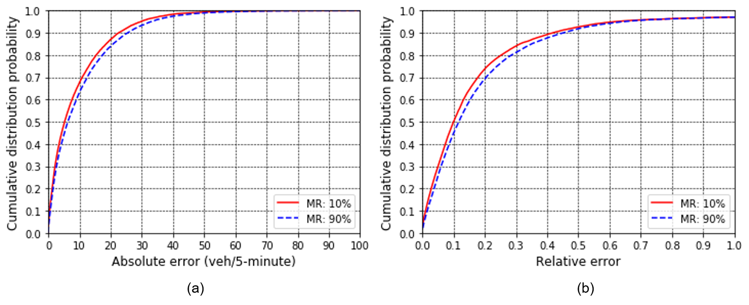
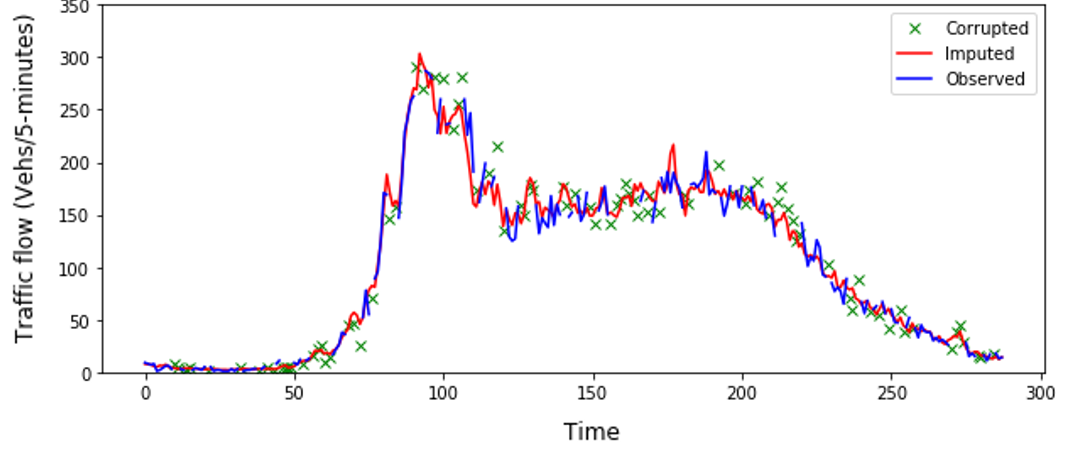
To extend this further, Figure 7 shows the absolute error () distribution and the relative error () distributions for 10% and 90% s. This can help to understand the and variation range within two extreme s (10% and 90%). It can be observed that about 60% of was less than 8 veh/5-mins at 10% , while it is less than 9 veh/5-mins at 90% . Similarly, there is about 60% of less than 13.5% at 10% , while it is less than 15.5% at 90% . By taking advantage of the generative model and temporal dependency correlation GASF matrix, our proposed model can produce robust and reliable imputation results even for large variation of s. A sample weekday and non-weekday imputation results is shown in Figure 8a and 8b, respectively. The figure shows the imputed data obtained using the proposed model along with the corresponding actual “observed" data and corrupted data too. It can be seen that the sample synthetic traffic flow data produced by our proposed model perform reliably well in successfully overlaying the observed part, with its “closest” estimation of the corrupted data points.


To illustrate the efficiency of our proposed model in learning the traffic data distribution, we plot the traffic flow histograms generated using the real data and the synthetic data obtained from the model for 20% , as shown in Figure 9a. Further, Figure 9b shows the empirical distributions of the deviation time series of the real data and the synthetically generated data, similar to Chen et al. 2012, Li et al. 2013. The deviations are calculated as difference between simple average intra-day trend from the original and imputed data. This helps to check if the imputed data preserve the important statistical features of the original dataset. As it can be seen from Figure 9(a) and (b), the synthetic data distributions closely follow the original data distributions, thereby verifying that the proposed imputation technique has been able to retain the original data features successfully. In the next section, we discuss the details of our proposed model performance in a large-scale implementation over the entire District 5 of California instead of a single sensor imputation.

4.4 Imputation Performance on a Large-Scale Network
In this subsection, we evaluate our proposed model using the entire 2013 data obtained from all VDSs of District 5 of California. As mentioned in Section 3.6, we first divided the 147 VDSs into different homogeneous groups based on their daily traffic flow patterns using the k-means and elbow method. As shown in Figure 10, we draw the sum of squared distances versus the possible number of clusters, and used the elbow method to determine the optimal number of clusters () [Kodinariya and Makwana 2013]. The optimal number of clusters were found to be 25 using the elbow point. However, the selection of the optimal groups can also be chosen based on the agency specific requirements.

To demonstrate the different daily patterns observed in the generated clusters, we plot the median daily traffic flow data of 5 sample clusters in Figure 11. The average daily traffic (ADT) for these 5 sample groups varied between 9,000 to 64,000 vehicles. It can be seen that there were both morning and evening peaks for groups 4 and 5, while groups 2 and 3 have either a morning peak or an evening peak. It can also be seen that group 1 had the lowest daily traffic flow. Therefore, the clusters generated having distinct traffic flow patterns help the model to learn those unique patterns and perform more efficiently in large-scale network.


In addition, to ensure fair and balanced results for each individual VDS, we selected 20% of the samples equally from each VDS for testing and used the remaining 80% for training. Figure 12 shows the performance of our proposed model for all VDS in a sample group 2 for MR ranging between 10% to 80%. It can be seen that for all VDSs ranging from 9.1 to 10.6 veh/5-mins, ranging from 12.9 to 15.3 veh/5-mins, and ranging from 17.1% to 23.6%. This shows that the proposed model scales efficiently for larger number of VDSs, in addition to the single VDS model described in Section 4.3.

Table 1 summarizes the overall performance of our proposed TSDIGAN model for the 5 sample clusters, whose daily pattern is shown in Figure 11. It can be seen that the model performed reasonably well even in high of 80%, showing the efficacy of the model. Further, although the and increased for clusters with higher , the showed decreasing trend with increase in , thereby showing it’s performance is robust for different ranges of too.
| Criteria | MAE (veh/5-min) | RMSE (veh/5-min) | MRE | ||||||||||
|---|---|---|---|---|---|---|---|---|---|---|---|---|---|
| Group | ADT | 20% | 50% | 80% | 20% | 50% | 80% | 20% | 50% | 80% | |||
| 1 | 9000 | 5.0 | 5.2 | 5.6 | 7.2 | 7.5 | 8.1 | 0.318 | 0.327 | 0.350 | |||
| 2 | 29000 | 9.5 | 9.7 | 10.4 | 13.8 | 14.0 | 15.0 | 0.191 | 0.200 | 0.216 | |||
| 3 | 30000 | 9.8 | 10.0 | 10.6 | 14.5 | 14.9 | 15.5 | 0.200 | 0.210 | 0.221 | |||
| 4 | 47000 | 13.9 | 14.1 | 15.2 | 19.8 | 20.4 | 21.7 | 0.119 | 0.124 | 0.133 | |||
| 5 | 64000 | 14.6 | 14.9 | 16.4 | 20.7 | 21.4 | 22.9 | 0.103 | 0.108 | 0.116 | |||
Figure 13 presents the imputation performance accuracies in terms of , , and for all 147 VDSs of the entire District 5 of California at 30% MR. For all VDSs, was found to vary between 7.61 to 31.55 veh/5-mins with the median and mean values of 12.64 and 13.16 veh/5-mins respectively. Similarly, varied between 10.91 to 52.9 veh/5-mins with the median and mean of 18.98 and 20.22 veh/5-mins respectively. Therefore, the proposed model performed reasonably well across large-scale sensor networks in terms of and . However, was found to vary between 12.4% to 469% with the median and mean values of 20.7% and 35.5%. Therefore, the performance for the proposed model was found to be highly skewed, with exceptionally high for VDS ID 126 and 127. On further investigation, it was observed that the input of raw training data of these sensors had more inherent noise and zero volume report which made learning of the sufficient representative “pattern" from such training data highly unstable. However, the median across all sensors were found to be only 20.7%, suggesting reasonable overall performance across the sensors. These results indicates that the efficiency of our proposed TSDIGAN framework across districtwide sensor networks, thereby showing it’s feasibility for large-scale practical implementations.

Additionally, efficiency of real-world implementation of the proposed model depends on the training and testing cost and time requirements. This is particularly important since training deep learning models is time-consuming and GANs in particular are well-known to suffer from vanishing gradients, mode collapse, and failure to convergence. Our proposed model was trained and tested using a single NVIDIA GTX 1080Ti GPU along with Intel(R) i7-8700 CPU, 32 GB RAM, and Windows 10 (64 bits) platform. All the frameworks used in this study were built using PyTorch 1.1 [Paszke et al. 2017]. Our proposed model took approximately 8 minutes training time for a single VDS and 14 hours for the entire districtwide 147 VDSs using one year of historical traffic flow data for 50 epochs. The average training time for each group of VDS obtained using clustering method is found to be around 30 minutes. To find the optimal latent space using the imputation module during the test phase, the time taken varies depending on the iterations. In our experiments, we performed 200 iterations which was found to take approximately 2 seconds for generating daily traffic data generation for a single VDS. Therefore, it takes approximately 5 minutes for districtwide daily traffic data imputation across 147 VDS. This shows that the proposed model can be successfully applied to large-scale real-world implementation scenarios with the desired regular offline model retrain/update. Next, we present the results on comparison of our proposed model with other benchmark data imputation models.
4.5 Model Comparison
In this section, we compare the performance of our proposed TSDIGAN model with other benchmark traffic data imputation models to find out the efficiency of our proposed model. The benchmark models used in this study for comparison are support vector regression (SVR), history average (HA), denoising stacked autoencoder (DSAE), and GAN based parallel data model [Chen et al. 2019]. It should be noted that the benchmark dataset used in our study was also used by Duan et al. 2016 for DSAE model and Chen et al. 2019 for GAN based parallel data model. This enabled us to directly compare the performance of our model with these benchmark models. The detailed default settings for model training and evaluation results for baseline models can be found in Chen et al. 2019. Figure 14 shows the average imputation performance accuracies across all VDS in terms of , , and for all comparison models. It can be seen that our proposed model outperformed all other benchmark models in terms of and . An overall improvement of 13.7 % and 16.3 % was observed by TSDIGAN model compared to the next best performing parallel data model. However, in terms of , the proposed TSDIGAN model performed poorly to other benchmark models, except SVR. This can be contributed due to a few sensors for which was found to be significantly higher, as shown in Figure 13 and described in Section 4.4. Further, while the benchmark models were trained individually for each sensor separately, we trained our models for each cluster or group of sensors which can be attributed to be one of the reason why our model performs poorly for sensors with significant noise or zero volume report compared to other sensors. It can be pointed out that while the mean for TSDIGAN across all sensors for 30% MR was found to be 35.5%, the median was only 20.7%. Also, the mean for 95% of sensors was found to vary between 24.0% - 26.1% in comparison to 35.5% - 39.4% variation, when all sensors are considered. This implies that the mean value shown in Figure 14 was significantly affected by performance on few outlying sensors, which led to its poor performance compared to other benchmark models. In future, more efficient clustering techniques can be used either to remove such sensors from performance analysis or separate models can be trained for such sensors, depending on user specific requirements. Overall, the proposed TSDIGAN model outperformed all benchmark models in terms of and , while performing reasonably well in terms of too for majority of sensors.

5 Conclusion
In this study, we propose a traffic sensor data imputation framework based on generative adversarial networks (TSDIGAN) that treats the missing data problem as a data generation problem. Our study demonstrates that the generative model based method can perform accurately and robustly to impute missing traffic data under widely varying missing rates. Our proposed model first embeds traffic time-series data into GASF matrix images preserving the temporal correlations. This enables training of a deep convolutional generative adversarial network that can generate realistic-looking synthetic data for missing data imputation. We have also shown our proposed model’s training process step by step, demonstrating how our model learns to generate its high-quality synthetic data. We have evaluated the performance of the proposed model using benchmark data from PeMS [PeMS 2014] and further investigated it’s capability for large-scale applications. We compared our proposed model performance with other benchmark models, including support vector regression (SVR), history average (HA), denoising stacked autoencoder (DSAE), and GAN-based parallel data model. Our results show that the proposed model can outperform the benchmark models in terms of and , while achieving comparable accuracies in terms of for majority of the sensors. Further, our proposed framework groups the sensors into clusters based on the similarity of their daily traffic patterns to learn the generative model which can be applied to the entire cluster. This can help to train fewer cluster-specific models instead of maintaining each sensor specific model, thereby handling the entire training, testing, and real-world application procedure more efficiently.
Our proposed framework can easily and cheaply generate a variety of realistic synthetic traffic data, which makes it a good choice when it is inconvenient or impossible to get sufficient real traffic data. In addition, the characteristics of our proposed framework offer the possibility of extended ITS applications like data analysis enhancement, anomaly detection, etc. In future, this can be integrated with external features such as weather, special events, and other factors that can impact traffic flow patterns to enable our model to provide more adaptive and accurate imputation performance to appropriately reflect different conditions. Further, in this study, we used k-means clustering to group the sensors based on their daily traffic patterns and develop models for each cluster. In future, this study can be extended to evaluate other efficient clustering techniques such as hierarchical clustering, density based clustering and even determining optimal variation of temporal and spatial traffic data characteristics which can be grouped and worked upon as a single cluster. Also, this can be extended to evaluate the suitability and effectiveness of such generative model based deep learning frameworks for traffic speed generation, prediction, and similar other ITS applications.
Acknowledgements
Our research results are based upon work supported by the Iowa DOT Office of Traffic Operations Support Grant. Any opinions, findings, and conclusions or recommendations expressed in this material is of the author(s) and do not necessarily reflect the views of the Iowa DOT Office of Traffic Operations.
References
- Al-Deek et al. [2004] Al-Deek, H.M., Venkata, C., Chandra, S.R., 2004. New algorithms for filtering and imputation of real-time and archived dual-loop detector data in i-4 data warehouse. Transportation research record 1867, 116–126.
- Allison [2001] Allison, P.D., 2001. Missing data. volume 136. Sage publications.
- Anandkumar et al. [2014] Anandkumar, A., Ge, R., Hsu, D., Kakade, S.M., Telgarsky, M., 2014. Tensor decompositions for learning latent variable models. The Journal of Machine Learning Research 15, 2773–2832.
- Armanious [2019] Armanious, A., 2019. District 07 Mobility Performance Report: 2018 Fourth Quarter. Technical Report. California Department of Transportation.
- Asadi and Regan [2019] Asadi, R., Regan, A., 2019. A convolution recurrent autoencoder for spatio-temporal missing data imputation. arXiv preprint arXiv:1904.12413 .
- Berkhin [2006] Berkhin, P., 2006. A survey of clustering data mining techniques, in: Grouping multidimensional data. Springer, pp. 25–71.
- Borji [2019] Borji, A., 2019. Pros and cons of gan evaluation measures. Computer Vision and Image Understanding 179, 41–65.
- Castro-Neto et al. [2009] Castro-Neto, M., Jeong, Y.S., Jeong, M.K., Han, L.D., 2009. Online-svr for short-term traffic flow prediction under typical and atypical traffic conditions. Expert systems with applications 36, 6164–6173.
- Chakraborty et al. [2018a] Chakraborty, P., Adu-Gyamfi, Y.O., Poddar, S., Ahsani, V., Sharma, A., Sarkar, S., 2018a. Traffic congestion detection from camera images using deep convolution neural networks. Transportation Research Record: Journal of the Transportation Research Board 2672, 222–231. doi:10.1177/0361198118777631.
- Chakraborty et al. [2019] Chakraborty, P., Hegde, C., Sharma, A., 2019. Data-driven parallelizable traffic incident detection using spatio-temporally denoised robust thresholds. Transportation research part C: emerging technologies 105, 81–99.
- Chakraborty et al. [2018b] Chakraborty, P., Sharma, A., Hegde, C., 2018b. Freeway traffic incident detection from cameras: A semi-supervised learning approach, in: 2018 21st International Conference on Intelligent Transportation Systems (ITSC), IEEE. pp. 1840–1845.
- Chang et al. [2012] Chang, G., Zhang, Y., Yao, D., 2012. Missing data imputation for traffic flow based on improved local least squares. Tsinghua Science and Technology 17, 304–309.
- Chen et al. [2012] Chen, C., Wang, Y., Li, L., Hu, J., Zhang, Z., 2012. The retrieval of intra-day trend and its influence on traffic prediction. Transportation research part C: emerging technologies 22, 103–118.
- Chen et al. [2019] Chen, Y., Lv, Y., Wang, F.Y., 2019. Traffic flow imputation using parallel data and generative adversarial networks. IEEE Transactions on Intelligent Transportation Systems .
- Cummins et al. [2017] Cummins, N., Amiriparian, S., Hagerer, G., Batliner, A., Steidl, S., Schuller, B.W., 2017. An image-based deep spectrum feature representation for the recognition of emotional speech, in: Proceedings of the 25th ACM international conference on Multimedia, pp. 478–484.
- Donahue et al. [2018] Donahue, C., McAuley, J., Puckette, M., 2018. Adversarial audio synthesis. arXiv preprint arXiv:1802.04208 .
- Duan et al. [2016] Duan, Y., Lv, Y., Liu, Y.L., Wang, F.Y., 2016. An efficient realization of deep learning for traffic data imputation. Transportation research part C: emerging technologies 72, 168–181.
- Esteban et al. [2017] Esteban, C., Hyland, S.L., Rätsch, G., 2017. Real-valued (medical) time series generation with recurrent conditional gans. arXiv preprint arXiv:1706.02633 .
- Gan et al. [2017] Gan, Q., Gomes, G., Bayen, A., 2017. Estimation of performance metrics at signalized intersections using loop detector data and probe travel times. IEEE Transactions on Intelligent Transportation Systems 18, 2939–2949.
- Ghosh et al. [2007] Ghosh, B., Basu, B., O’Mahony, M., 2007. Bayesian time-series model for short-term traffic flow forecasting. Journal of transportation engineering 133, 180–189.
- Goodfellow et al. [2016] Goodfellow, I., Bengio, Y., Courville, A., 2016. Deep learning. MIT press.
- Goodfellow et al. [2014] Goodfellow, I., Pouget-Abadie, J., Mirza, M., Xu, B., Warde-Farley, D., Ozair, S., Courville, A., Bengio, Y., 2014. Generative adversarial nets, in: Advances in neural information processing systems, pp. 2672–2680.
- Gretton et al. [2007] Gretton, A., Borgwardt, K., Rasch, M., Schölkopf, B., Smola, A.J., 2007. A kernel method for the two-sample-problem, in: Advances in neural information processing systems, pp. 513–520.
- Isola et al. [2017] Isola, P., Zhu, J.Y., Zhou, T., Efros, A.A., 2017. Image-to-image translation with conditional adversarial networks, in: Proceedings of the IEEE conference on computer vision and pattern recognition, pp. 1125–1134.
- Kim et al. [2018] Kim, Y., Wang, P., Zhu, Y., Mihaylova, L., 2018. A capsule network for traffic speed prediction in complex road networks, in: 2018 Sensor Data Fusion: Trends, Solutions, Applications (SDF), IEEE. pp. 1–6.
- Kodinariya and Makwana [2013] Kodinariya, T.M., Makwana, P.R., 2013. Review on determining number of cluster in k-means clustering. International Journal 1, 90–95.
- Ku et al. [2016] Ku, W.C., Jagadeesh, G.R., Prakash, A., Srikanthan, T., 2016. A clustering-based approach for data-driven imputation of missing traffic data, in: 2016 IEEE Forum on Integrated and Sustainable Transportation Systems (FISTS), IEEE. pp. 1–6.
- LeCun et al. [1998] LeCun, Y., Bottou, L., Bengio, Y., Haffner, P., et al., 1998. Gradient-based learning applied to document recognition. Proceedings of the IEEE 86, 2278–2324.
- Ledig et al. [2017] Ledig, C., Theis, L., Huszár, F., Caballero, J., Cunningham, A., Acosta, A., Aitken, A., Tejani, A., Totz, J., Wang, Z., et al., 2017. Photo-realistic single image super-resolution using a generative adversarial network, in: Proceedings of the IEEE conference on computer vision and pattern recognition, pp. 4681–4690.
- Lee et al. [2019] Lee, D., Kim, J., Moon, W.J., Ye, J.C., 2019. Collagan: Collaborative gan for missing image data imputation, in: Proceedings of the IEEE Conference on Computer Vision and Pattern Recognition, pp. 2487–2496.
- Lee and Coifman [2011] Lee, H., Coifman, B., 2011. Quantifying loop detector sensitivity and correcting detection problems on freeways. Journal of Transportation Engineering 138, 871–881.
- Lefebvre et al. [2017] Lefebvre, N., Chen, X., Beauseroy, P., Zhu, M., 2017. Traffic flow estimation using acoustic signal. Engineering Applications of Artificial Intelligence 64, 164–171.
- Li et al. [2019] Li, D., Chen, D., Jin, B., Shi, L., Goh, J., Ng, S.K., 2019. Mad-gan: Multivariate anomaly detection for time series data with generative adversarial networks, in: International Conference on Artificial Neural Networks, Springer. pp. 703–716.
- Li et al. [2013] Li, L., Li, Y., Li, Z., 2013. Efficient missing data imputing for traffic flow by considering temporal and spatial dependence. Transportation research part C: emerging technologies 34, 108–120.
- Li et al. [2014] Li, Y., Li, Z., Li, L., 2014. Missing traffic data: comparison of imputation methods. IET Intelligent Transport Systems 8, 51–57.
- Lu et al. [2017] Lu, L., Wang, J., He, Z., Chan, C.Y., 2017. Real-time estimation of freeway travel time with recurrent congestion based on sparse detector data. IET Intelligent Transport Systems 12, 2–11.
- Luo et al. [2018] Luo, Y., Cai, X., Zhang, Y., Xu, J., et al., 2018. Multivariate time series imputation with generative adversarial networks, in: Advances in Neural Information Processing Systems, pp. 1596–1607.
- Lv et al. [2018] Lv, Y., Chen, Y., Li, L., Wang, F.Y., 2018. Generative adversarial networks for parallel transportation systems. IEEE Intelligent Transportation Systems Magazine 10, 4–10.
- Lv et al. [2014] Lv, Y., Duan, Y., Kang, W., Li, Z., Wang, F.Y., 2014. Traffic flow prediction with big data: a deep learning approach. IEEE Transactions on Intelligent Transportation Systems 16, 865–873.
- Ma et al. [2017] Ma, D., Luo, X., Li, W., Jin, S., Guo, W., Wang, D., 2017. Traffic demand estimation for lane groups at signal-controlled intersections using travel times from video-imaging detectors. IET Intelligent Transport Systems 11, 222–229.
- MacQueen et al. [1967] MacQueen, J., et al., 1967. Some methods for classification and analysis of multivariate observations, in: Proceedings of the fifth Berkeley symposium on mathematical statistics and probability, Oakland, CA, USA. pp. 281–297.
- Ni and Leonard [2005] Ni, D., Leonard, J.D., 2005. Markov chain monte carlo multiple imputation using bayesian networks for incomplete intelligent transportation systems data. Transportation research record 1935, 57–67.
- Nihan [1997] Nihan, N.L., 1997. Aid to determining freeway metering rates and detecting loop errors. Journal of Transportation Engineering 123, 454–458.
- Park et al. [1998] Park, B., Messer, C.J., Urbanik, T., 1998. Short-term freeway traffic volume forecasting using radial basis function neural network. Transportation Research Record 1651, 39–47.
- Paszke et al. [2017] Paszke, A., Gross, S., Chintala, S., Chanan, G., Yang, E., DeVito, Z., Lin, Z., Desmaison, A., Antiga, L., Lerer, A., 2017. Automatic differentiation in pytorch, in: NIPS-W.
- PeMS [2014] PeMS, 2014. Pems. http://pems.dot.ca.gov/. Accessed June, 2014.
- Qu et al. [2009] Qu, L., Li, L., Zhang, Y., Hu, J., 2009. Ppca-based missing data imputation for traffic flow volume: A systematical approach. IEEE Transactions on intelligent transportation systems 10, 512–522.
- Radford et al. [2015] Radford, A., Metz, L., Chintala, S., 2015. Unsupervised representation learning with deep convolutional generative adversarial networks. arXiv preprint arXiv:1511.06434 .
- Salimans et al. [2016] Salimans, T., Goodfellow, I., Zaremba, W., Cheung, V., Radford, A., Chen, X., 2016. Improved techniques for training gans, in: Advances in neural information processing systems, pp. 2234–2242.
- Shi and Abdel-Aty [2015] Shi, Q., Abdel-Aty, M., 2015. Big data applications in real-time traffic operation and safety monitoring and improvement on urban expressways. Transportation Research Part C: Emerging Technologies 58, 380–394.
- Smith et al. [2003] Smith, B.L., Scherer, W.T., Conklin, J.H., 2003. Exploring imputation techniques for missing data in transportation management systems. Transportation Research Record 1836, 132–142.
- Susmelj et al. [2017] Susmelj, I., Agustsson, E., Timofte, R., 2017. Abc-gan: Adaptive blur and control for improved training stability of generative adversarial networks, in: International Conference on Machine Learning (ICML 2017) Workshop on Implicit Models.
- Tan et al. [2013] Tan, H., Feng, G., Feng, J., Wang, W., Zhang, Y.J., Li, F., 2013. A tensor-based method for missing traffic data completion. Transportation Research Part C: Emerging Technologies 28, 15–27.
- Wang and Oates [2015] Wang, Z., Oates, T., 2015. Encoding time series as images for visual inspection and classification using tiled convolutional neural networks, in: Workshops at the Twenty-Ninth AAAI Conference on Artificial Intelligence.
- Wang et al. [2017] Wang, Z., Yan, W., Oates, T., 2017. Time series classification from scratch with deep neural networks: A strong baseline, in: 2017 international joint conference on neural networks (IJCNN), IEEE. pp. 1578–1585.
- Yeh et al. [2017] Yeh, R.A., Chen, C., Yian Lim, T., Schwing, A.G., Hasegawa-Johnson, M., Do, M.N., 2017. Semantic image inpainting with deep generative models, in: Proceedings of the IEEE Conference on Computer Vision and Pattern Recognition, pp. 5485–5493.
- Yin et al. [2012] Yin, W., Murray-Tuite, P., Rakha, H., 2012. Imputing erroneous data of single-station loop detectors for nonincident conditions: Comparison between temporal and spatial methods. Journal of Intelligent Transportation Systems 16, 159–176.
- Yu et al. [2018] Yu, J., Lin, Z., Yang, J., Shen, X., Lu, X., Huang, T.S., 2018. Generative image inpainting with contextual attention, in: Proceedings of the IEEE Conference on Computer Vision and Pattern Recognition, pp. 5505–5514.
- Zhao et al. [2018] Zhao, H., Gan, C., Rouditchenko, A., Vondrick, C., McDermott, J., Torralba, A., 2018. The sound of pixels, in: Proceedings of the European Conference on Computer Vision (ECCV), pp. 570–586.
- Zhuang et al. [2018] Zhuang, Y., Ke, R., Wang, Y., 2018. Innovative method for traffic data imputation based on convolutional neural network. IET Intelligent Transport Systems 13, 605–613.