A Heuristic Based on Randomized Greedy Algorithms for the Clustered Shortest-Path Tree Problem
Abstract
Randomized Greedy Algorithms (RGAs) are interesting approaches to solve problems whose structures are not well understood as well as problems in combinatorial optimization which incorporate the random processes and the greedy algorithms. This paper introduces a new algorithm that combines the major features of RGAs and Shortest Path Tree Algorithm (SPTA) to deal with the Clustered Shortest-Path Tree Problem (CluSPT). In our algorithm, SPTA is used to determine the shortest path tree in each cluster while the combination between characteristics of the RGAs and search strategy of SPTA is used to constructed the edges connecting clusters. To evaluate the performance of the proposed algorithm, Euclidean benchmarks are selected. The experimental investigations show the strengths of the proposed algorithm in comparison with some existing algorithms. We also analyze the influence of the parameters on the performance of the algorithm.
Index Terms:
Randomized Greedy Algorithms, Clustered Shortest-Path Tree Problem, Random Optimization, Random Search Heuristics, Shortest Path Tree Algorithm.I Introduction
The incorporation of randomness in many algorithms can be crucial to solve various problems in the fields of computer sciences. For example, one of the most well-known algorithms in randomized search heuristics [1, 2] is Evolutionary Algorithm (EA) [3] which is successfully applied to deal with numerous type of problems. In EA [4, 5], the randomness appears in most of key components of the algorithms such as the process of population initialization, the crossover and mutation operators. Another remarkable algorithm is Ant Colony Optimization (ACO) [6] which currently also attracts a lot of attention in the scientific community to extend and apply to many hard optimization problems. In ACO, the randomness is used to construct ant solutions [6].
Recently, some variants of heuristic search algorithms are proposed such as Greedy Randomized Adaptive Search Procedure (GRASP) [7, 8], RGAs [9, 10, 11], etc. in which RGAs are notable approaches because of the fact that RGAs takes both advantages of the Greedy Algorithm (fast approach for finding a solution, and implementation in a very simple way [9]) and random search methods (simple implementation, easy computation; effective when constraints are involved or the gradient is burdensome [1]). RGAs randomizes the greedy step to prevent the algorithm from producing bad solutions. A major difference in comparison with deterministic greedy algorithm is that RGAs selects a solution component from a set of available components at each step according to the given probability distribution. Therefore, RGAs use an additional parameter () to compute the amount of greediness. RGAs has been proved to be effective when solving some problems [9, 10, 11].
Nowadays, the problem of communication network connection arises as an urgent demand. As a result, clustered tree problems such as the Clustered Steiner Tree problem, the Inter Cluster Tree Problem and the CluSPT also attract a lot of interests for their wide range of applications. In particular, the CluSPT has some applications such as: goods distribution, water supplies, and fiber optic cable network.
There have been some studies to deal with the CluSPT. Those studies are based on the Multifactorial Evolutionary Algorithm (MFEA) and focused on searching solutions of many problems simultaneously. Although those algorithms have been proven to be effective in some test cases, in the aspect of producing a good solution that approximates the global optimum within a small amount of time, the existing algorithms have revealed some restrictions.
As a consequence, we propose a random heuristic search for the CluSPT. The proposed algorithm is a combination between RGAs and SPTA. The main objective of the SPTA is to construct the shortest-path tree for each cluster while the objective of RGAs is to build the edges connecting the clusters. To select an edge to connect a visited cluster to an unvisited cluster, our algorithm, Heuristic Based on Randomized Greedy Algorithm (HBRGA), defines a reward of an edge based on the weight of the edge and the cost of the shortest-path tree of the unvisited cluster rooted at one end of the edge. Then, HBRGA selects an edge according to a probabilistic distribution formula which is computed based on the rewards of the edges. Extensive computational results are reported and discussed for various Euclidean benchmarks. The obtained results demonstrate the efficiency of our approach compared to some existing methods.
The major contributions of this work as following:
- •
Propose a mechanism for combining the RGAs with the SPTA to deal with the CluSPT.
- •
Suggest a strategy for evaluating rewards of edges.
- •
Introduce a random effect during the edge selection to construct temporary solution.
- •
Analyze the effects of parameters on the performance of the proposed algorithm.
- •
Experiment to evaluate the efficiency of the proposed algorithm.
II Notation and definitions
In this paper, we consider simple connected undirected graphs. For a graph , is the vertex set, is the edge set, and is the nonnegative edge length function of the graph. The weight of an edge (u, v) is denoted by .
For a graph , and denote the vertex and the edge sets, respectively. For a vertex subset , the sub-graph of induced by is denoted by . For a vertex set , a collection of subsets of is a partition of if the subsets are mutually disjoint and their union is exactly . A path of is simple if no vertex appears more than once on the path. In this paper we consider only simple paths.
is the set of all the clusters that have not been included in the current solution. At the beginning, contains all k clusters.
Root cluster is the cluster that has the source vertex.
Local root of a cluster is the first vertex on the path from the source vertex to a vertex in that cluster. Let be the local root of cluster .
The distance between the root cluster and another cluster is defined by the total cost of the shortest path from the source vertex to the local root of that cluster. Let be the distance from the root cluster to cluster , so we first initialize:
- •
,
- •
,
For each cluster , is the distance from the local root of cluster to a vertex .
For a given spanning tree of and , let denote the shortest path length between and on .
The CluSPT is defined as following:
| Input: | - A weighted undirected graph . |
|---|---|
| - Vertex set is partitioned into clusters . | |
| - A source vertex . | |
| Output: | - A spanning tree of . |
| - Sub-graph is a connected graph. | |
| Objective: | min |
III Related works
Randomized search heuristics are successfully applied to various types of problems, especially for the problems having not well-understood structure or problems in combinatorial optimization [3], such as EA for Traveling Salesman Problem (TSP) [12] and Capacitated Vehicle Routing Problem (CVRP) [13]; simulated annealing for CVRP [14]; GRASP for quadratic assignment problem [15], for Steiner problem [16] and for generalized minimum spanning tree problem [17]; RGAs for Covering Problems [9] and Maximum Matching Problem [10, 18]; etc. Each algorithm has its own advantages but in the aspect of looking for good approximations of optimal solutions within a small amount of time and easy to implement, the RGAs are one of the most suitable approaches.
The conception of RGAs is inspired from incorporating randomness into greedy algorithm. In RGAs, randomness is used in greedy selection steps [9] for improving the quality of solutions. RGAs proves to be effective in solving various types of problems.
Yuan Zhang et.al. [11] introduced a randomized greedy algorithm for dependency parsing. The main benefit of proposed algorithm is to tie to the number of local maxima in the search space. The authors point out that a randomized greedy method of inference surpasses the state-of-art performance in dependency parsing.
In [19], a randomized version of the greedy algorithm is presented to determine a large matching in a graph. The authors point out that on some classes of sparse graphs, RGAs performs significantly better than the worst-case and the ratio of the expected size of the randomized greedy matching to maximum size of matching is at least 0.7690. J. Aronson et.al. [18] considered the modified randomized greedy algorithm for finding a matching M in an arbitrary graph. The authors proved that the maximum matching within a factor of at leats . The authors also received stronger results for tree and sparse graphs. Mathhias Poloczek et.al. [10] invented the Constrast Analysis technique to analyze the lower bound of the modified randomized greedy algorithm (MRGA) [18] for the Maximum Matching Problem. The authors proved that the lower bound of approximation ratio of the MRGA is for any graph.
The network optimization problems have important roles in various applications in daily-life [20, 21], in which some problems have clustered structure [20]. Therefore, clustered problems are being received many interests in the scientific community. One of the newest clustered tree problem is the CluSPT which is formulated by M. D’Emidio et.al. [20]. Due to the fact that CluSPT is a NP-Hard problem [20], the meta-heuristic algorithms are often considered to look for the optimal solutions.
Recently, two algorithms based on the MFEA are proposed to find solutions for some input graph at a time. Those algorithms encode solutions of CluSPT by difference representations i.e. C-MFEA [22] uses the Cayley code while E-MFEA [23] uses edge-set to represent the solution. The major goal of C-MFEA is to determine CluSPT solution in short time while E-MFEA focuses on quality of solutions. The experimental results show that E-MFEA and C-MFEA outperform an existing algorithm.
Although some studies have been done to produce a good solution of CluSPT. However, in the aspect of finding a good solution within a small amount of time, the existing algorithms are not capable, so we have studied the combination of RGAs and SPTA then applied it for the CluSPT.
IV Proposed Algorithm
In this section, we introduce the mechanism of HBRGA and explain in detail how that algorithm works through an example.
IV-A Algorithmic skeleton of HBRGA
- 1.
Step 1: For the root cluster
- •
Step 1.1: Apply the Dijsktra’s algorithm from the source vertex to obtain the shortest-path tree of the root cluster.
- •
Step 1.2: Add the received tree in the root cluster to the solution and mark the root cluster as current cluster .
- •
Step 1.3: Exclude the root cluster from the set Q.
- •
- 2.
Step 2: For other clusters
The algorithm will add the remaining clusters one by one into the temporary solution/tree by applying the following steps:- •
Step 2.1: Finding a temporary edge connecting 2 clusters
For each cluster left in , find an edge that connects it and the current cluster by our proposed RGA. ( belongs to the current cluster, belongs to one remaining cluster ) - •
Step 2.2: Updating the distance between the root cluster and each cluster :
Let be the weight of the edge connecting 2 clusters in step 1. If , then and set . - •
Step 2.3:
- –
Find a cluster that has the minimum value of , and then add that cluster into the temporary solution/tree using the connecting edge in step 1.
- –
The spanning tree in cluster is created by applying the Dijsktra’s algorithm from the local root of obtained in step 2.
- –
Set as current cluster and exclude from the set .
- –
- •
Step 2.4: If is not empty, go to step 1. Otherwise, the algorithm stops.
- •
IV-B Algorithmic skeleton of proposed RGA
The proposed RGA is used to evaluate all clusters left in for updating the distance from each cluster to the root cluster.
For each remaining cluster in :
- •
Generate a random number that has the value between the number of vertices in Vi and the total number of vertices left in where is the cluster left in , is number of vertices in cluster ).
- •
Let be the set of all edges connecting the current cluster and a cluster . Define a function:
where is the total cost of the shortest paths from to other vertices in .
- •
The probability that an edge is chosen to connect the current cluster and a cluster is:
where is a parameter that determines the amount of greediness.
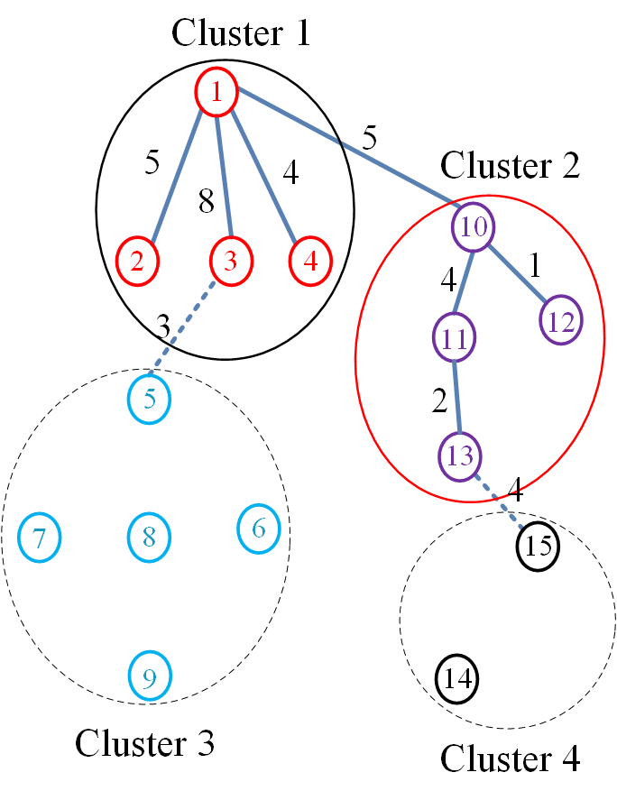
Figure 1 illustrates steps of the proposed algorithm in which Figure 1(a) presents input graph with source vertex as 1.
- •
Figure 1(b) illustrates the Step 1 and Step 2.1, in which the sub-graph of cluster 1 is obtained after finishing Step 1. In Step 2.1, HBRGA performs:
- –
Consider the edges connecting the current cluster (in red) which is cluster 1 and the remaining clusters (in dashed circle).
- –
There are 2 edges that connect cluster 1 and cluster 2 which are edge (1, 10) and edge (4, 11). Suppose HBRGA chooses the edge (1, 10) as a temporary edge to connect cluster 1 and cluster 2.
- –
Since there is only one edge that connect cluster 1 and cluster 3, the edge (3, 5) is chosen to be a temporary edge to connect those clusters.
- –
- •
Figure 1(c) illustrates the Step 2.3 when:
- –
Since the distance between cluster 1 and cluster 2 is 5 and between cluster 1 and cluster 3 is 8 + 3 = 11, cluster 2 is set as current cluster and the edge (1, 10) is added to the temporary solution.
- –
Add the shortest-path tree of cluster 2 by the Dijkstra’s algorithm with the start vertex as 10 to the temporary solution.
- –
- •
Figure 1(d) illustrates the Step 2.1 where cluster 2 is current cluster. Since the edge (13, 6) and edge (13, 15) connect cluster 2 and cluster 3, cluster 4 respectively, those edges are used to compute the distance from cluster 3 and cluster 4 to the root cluster.
- •
Figure 1(e) illustrates the Step 2.2 when:
- –
Update the distance from each unvisited cluster to root cluster (cluster 1)
- –
There are 2 edges connecting cluster 3 and the clusters that were added into the solution at previous steps (edge (3, 5) for cluster 1 and edge (6, 13) for cluster 2). Since the length of the shortest path from vertex 5 to source vertex 1 is 3 + 8 = 11 while the length of the shortest path from vertex 6 to source vertex 1 is 5 + 2 + 4 + 5 = 16, edge (3, 5) is kept to evaluate in next steps.
- –
- •
- •
- •
Figure 1(h) illustrates the complete solution for the CluSPT.




The Pseudocode of HBRGA is presented in Algorithm 1.
In Algorithm 1, method construct shortest path tree by using Dijkstra Algorithm with start vertex as . The method computes total cost of the shortest path from vertex to all vertices
V Computational results
V-A Problem instances
For assessment of the proposed algorithms’ performance, we created instances for the CluSPT from Clustered Traveling Salesman Problem (CluTSP) instances [24][25] by adding the information of the source vertex. The main reason for building CluSPT instances from CluTSP instances was that CluTSP instances had been generated with various algorithms to be suitable for clustered problems [25].
For evaluation of the proposed algorithms, small instances of CluTSP were selected for the building of instances for CluSPT.
All tested instances are available via [26].
V-B Experimental setup
We focused on the following criteria to assess the quality of the output of the algorithms.
| Criteria | |
|---|---|
| Average (Avg) | Average function value over all runs |
| Best-found (BF) | Best function value achieved over all runs |
To compare the effectiveness of the two algorithms, we evaluated the difference between the costs of the results obtained by the two algorithms A and B by the following formula:
where and denote the costs of the best solutions generated by A and B respectively.
To evaluate the performance of the MFEA in solving the CluSPT, we implemented two sets of experiments.
-
In the second set, various experiments were performed to analyze possible influencing factors.
Each problem instance was evaluated 30 times on Intel Core i7-3.60GHz, 16GB RAM computer using Windows 8 64-bit. The source codes were written in the Visual C# language.
V-C Experimental results
V-C1 Analysis of the parameter
Table I demonstrates the results of HBRGA with regards to different values of . These results indicate that, for complete graph, larger values of tend to give better results. In other words, the more greedy our algorithm becomes, the better results it would produce.
Hence, in this paper, we select the results when = 50 to compare our heuristic with some other existing algorithms.
V-C2 Comparison between the performance of existing algorithms and that of the proposed algorithm
In this section, the comparison between the results received by the HBRGA and those of 2 other existing algorithms (E-MFEA and C-MFEA) will be discussed. Table II, III and IV illustrate the results achieved by all 3 algorithms on instances of Type 1, Type 5 and Type 6 respectively. In those tables, the symbol ”-” indicates that the corresponding instances are not considered.
In general, the results obtained by HBRGA were considerably better in quality than those obtained by the C-MFEA and the E-MFEA in all test cases of the Type 1, Type 5 and Type 6.
As is observed in Table II, the proposed algorithm exceeded the E-MFEA on all instances in Type 1 with an average PI(HBRGA, E-MFEA) of 15.9%. In particluar, the highest PI(HBRGA, E-MFEA) was 39.2% on instance 10st70. Results obtained by the 2 algorithms on instances in Type 5 and Type 6 are presented in Table III, IV. The average PI(HBRGA, E-MFEA) was under one fifth on both types with the highest PI(HBRGA, E-MFEA) of Type 5 and Type 6 were 32.8% and 37.9% respectively.
In comparison with the C-MFEA, it is clear that the HBRGA outperformed it significantly on all test cases. The average PI(HBRGA, C-MFEA) obtained from each of the 3 types was above 40% with the greatest PI(HBRGA, C-MFEA) was 64.5% on instance 4pr76-2x2 in Type 6.
VI Conclusion
In this paper, we proposed a new heuristic based on the combination between RGA and SPTA to solve the CluSPT. To evaluate its effectiveness, the heuristic has been experimented on multiple types of Euclidean instances. The results have strongly proven the efficiency of our proposed heuristic. In the future, we will continue to analyze the results of the heuristic for many other types of graphs (Non-Euclidean, Sparse graph). Furthermore, we will add the shortest path tree cost factor into the formula evaluating the path from the root cluster to another cluster, in order to optimize the the cost of its spanning tree.
References
- [1] J. Li and R. R. Rhinehart, “Heuristic random optimization,” Computers & chemical engineering, vol. 22, no. 3, pp. 427–444, 1998.
- [2] M. D. Vose, “Random heuristic search,” Theoretical Computer Science, vol. 229, no. 1-2, pp. 103–142, 1999.
- [3] F. Neumann and I. Wegener, “Randomized local search, evolutionary algorithms, and the minimum spanning tree problem,” Theoretical Computer Science, vol. 378, no. 1, pp. 32–40, 2007.
- [4] E. E. Agoston, Introduction to Evolutionary Computing. Berlin, Springer-Verlag, 2003.
- [5] T. Back, Evolutionary algorithms in theory and practice: evolution strategies, evolutionary programming, genetic algorithms. Oxford university press, 1996.
- [6] M. Dorigo and T. Stützle, “Ant colony optimization: overview and recent advances,” in Handbook of metaheuristics. Springer, 2019, pp. 311–351.
- [7] A. E. Márquez and C. Expósito-Izquierdo, “An Overview of the Last Advances and Applications of Greedy Randomized Adaptive Search Procedure,” in Handbook of Research on Modeling, Analysis, and Application of Nature-Inspired Metaheuristic Algorithms. IGI Global, 2018, pp. 264–284.
- [8] M. G. Resende and C. C. Ribeiro, “GRASP: Greedy randomized adaptive search procedures,” in Search methodologies. Springer, 2014, pp. 287–312.
- [9] W. Gao, T. Friedrich, F. Neumann, and C. Hercher, “Randomized Greedy Algorithms for Covering Problems,” 2018.
- [10] M. Poloczek and M. Szegedy, “Randomized greedy algorithms for the maximum matching problem with new analysis,” in Foundations of Computer Science (FOCS), 2012 IEEE 53rd Annual Symposium on. IEEE, 2012, pp. 708–717.
- [11] Y. Zhang, T. Lei, R. Barzilay, and T. Jaakkola, “Greed is good if randomized: New inference for dependency parsing,” 2014.
- [12] Y. Nagata, “New EAX crossover for large TSP instances,” in Parallel Problem Solving from Nature-PPSN IX. Springer, 2006, pp. 372–381.
- [13] ——, “Edge Assembly Crossover for the Capacitated Vehicle Routing Problem,” in Evolutionary Computation in Combinatorial Optimization: 7th European Conference, EvoCOP 2007, Valencia, Spain, April 11-13, 2007. Proceedings, C. Cotta and J. Hemert, Eds. Berlin, Heidelberg: Springer Berlin Heidelberg, 2007, pp. 142–153. [Online]. Available: http://dx.doi.org/10.1007/978-3-540-71615-0_13
- [14] L. Wei, Z. Zhang, D. Zhang, and S. C. Leung, “A simulated annealing algorithm for the capacitated vehicle routing problem with two-dimensional loading constraints,” European Journal of Operational Research, vol. 265, no. 3, pp. 843–859, 2018.
- [15] G. R. Mateus, M. G. Resende, and R. M. Silva, “GRASP with path-relinking for the generalized quadratic assignment problem,” Journal of heuristics, vol. 17, no. 5, pp. 527–565, 2011.
- [16] C. C. Ribeiro, E. Uchoa, and R. F. Werneck, “A hybrid GRASP with perturbations for the Steiner problem in graphs,” INFORMS Journal on Computing, vol. 14, no. 3, pp. 228–246, 2002.
- [17] C. S. Ferreira, L. S. Ochi, V. Parada, and E. Uchoa, “A GRASP-based approach to the generalized minimum spanning tree problem,” Expert Systems with Applications, vol. 39, no. 3, pp. 3526–3536, 2012.
- [18] J. Aronson, M. Dyer, A. Frieze, and S. Suen, “Randomized greedy matching. II,” Random Structures & Algorithms, vol. 6, no. 1, pp. 55–73, 1995.
- [19] M. Dyer and A. Frieze, “Randomized greedy matching,” Random Structures & Algorithms, vol. 2, no. 1, pp. 29–45, 1991.
- [20] M. D’Emidio, L. Forlizzi, D. Frigioni, S. Leucci, and G. Proietti, “On the Clustered Shortest-Path Tree Problem.” in ICTCS, 2016, pp. 263–268.
- [21] C.-W. Lin and B. Y. Wu, “On the minimum routing cost clustered tree problem,” Journal of Combinatorial Optimization, pp. 1–16, 2016.
- [22] P. D. Thanh, D. A. Dung, T. N. Tien, and H. T. T. Binh, “An effective representation scheme in multifactorial evolutionary algorithm for solving cluster shortest-path tree problem,” in Evolutionary Computation (CEC), 2018 IEEE Congress on. IEEE, 2018, pp. 811–818.
- [23] H. T. T. Binh, P. D. Thanh, T. B. Trung, and L. P. Thao, “Effective multifactorial evolutionary algorithm for solving the cluster shortest path tree problem,” in Evolutionary Computation (CEC), 2018 IEEE Congress on. IEEE, 2018, pp. 819–826.
- [24] K. Helsgaun, “Solving the Clustered Traveling Salesman Problem Using the Lin-Kernighan-Helsgaun Algorithm,” Computer Science Research Report, no. 142, pp. 1–16, 2011.
- [25] M. Mestria, L. S. Ochi, and S. de Lima Martins, “GRASP with path relinking for the symmetric euclidean clustered traveling salesman problem,” Computers & Operations Research, vol. 40, no. 12, pp. 3218–3229, 2013.
- [26] P. D. Thanh, “CluSPT instances.” Mendeley Data v2, http://dx.doi.org/10.17632/b4gcgybvt6.2, 2018.
| Instances | = 1 | = 5 | = 10 | = 20 | = 30 | = 40 | = 50 | |||||||
|---|---|---|---|---|---|---|---|---|---|---|---|---|---|---|
| BF | Avg | BF | Avg | BF | Avg | BF | Avg | BF | Avg | BF | Avg | BF | Avg | |
| 10berlin52 | 45828.6 | 48866.6 | 44303.5 | 46428.2 | 44042.3 | 45325.5 | 43802.7 | 44500.4 | 43724.1 | 44214.5 | 43738.6 | 44002.0 | 43738.6 | 43971.0 |
| 10eil51 | 2009.8 | 2297.3 | 1733.9 | 1837.8 | 1713.3 | 1760.9 | 1713.2 | 1729.4 | 1713.2 | 1725.1 | 1713.2 | 1723.8 | 1713.2 | 1723.2 |
| 10eil76 | 2596.4 | 3562.5 | 2249.4 | 2426.2 | 2204.0 | 2254.1 | 2203.3 | 2217.7 | 2203.3 | 2210.1 | 2203.3 | 2209.1 | 2203.3 | 2208.4 |
| 10kroB100 | 160439.5 | 188533.8 | 148188.4 | 161012.6 | 145243.6 | 150565.0 | 141824.9 | 145118.9 | 140820.0 | 142994.3 | 140653.5 | 142257.6 | 140635.1 | 141951.4 |
| 10pr76 | 605003.0 | 674451.2 | 565285.7 | 592198.8 | 532573.4 | 555253.6 | 523893.3 | 534672.9 | 523249.0 | 529046.4 | 522572.2 | 527656.6 | 522572.2 | 525733.1 |
| 10rat99 | 9008.3 | 10210.9 | 7925.8 | 8466.1 | 7621.9 | 7888.7 | 7520.2 | 7653.7 | 7520.2 | 7603.2 | 7520.2 | 7576.8 | 7520.2 | 7562.1 |
| 10st70 | 3543.5 | 4335.9 | 3174.3 | 3467.3 | 3117.0 | 3219.3 | 3099.2 | 3151.2 | 3099.5 | 3139.2 | 3099.5 | 3132.6 | 3099.5 | 3131.7 |
| 15berlin52 | 28984.6 | 32028.9 | 26974.8 | 28433.5 | 26522.0 | 27214.6 | 26346.0 | 26662.9 | 26345.5 | 26543.2 | 26312.1 | 26458.3 | 26312.0 | 26437.7 |
| 15eil51 | 1492.4 | 1632.2 | 1355.7 | 1436.7 | 1312.3 | 1359.2 | 1309.9 | 1325.6 | 1306.8 | 1318.5 | 1306.7 | 1317.3 | 1306.7 | 1313.8 |
| 15eil76 | 3236.2 | 3503.8 | 2993.3 | 3137.4 | 2957.2 | 3011.0 | 2918.3 | 2955.9 | 2914.4 | 2933.6 | 2911.3 | 2925.3 | 2911.3 | 2921.8 |
| 15pr76 | 771109.3 | 816189.0 | 732956.0 | 755924.1 | 718439.4 | 730875.2 | 708266.2 | 716625.6 | 707937.9 | 712899.3 | 706060.3 | 710154.1 | 705017.3 | 708944.9 |
| 15st70 | 4504.0 | 4826.7 | 4294.8 | 4452.4 | 4208.0 | 4311.8 | 4152.5 | 4207.8 | 4134.7 | 4177.1 | 4130.9 | 4155.6 | 4129.9 | 4147.3 |
| 25eil101 | 4901.3 | 5081.4 | 4715.2 | 4775.5 | 4698.0 | 4721.7 | 4683.9 | 4694.1 | 4683.4 | 4688.9 | 4680.8 | 4687.5 | 4680.8 | 4686.1 |
| 25kroA100 | 161039.3 | 172263.7 | 151282.7 | 157622.0 | 149080.1 | 151413.1 | 147698.6 | 148699.5 | 147430.1 | 148123.1 | 147300.8 | 147901.0 | 147239.0 | 147716.8 |
| 25lin105 | 107095.9 | 114122.6 | 102464.3 | 105958.3 | 99662.0 | 101742.0 | 98523.0 | 99646.7 | 98372.8 | 98946.4 | 98222.0 | 98680.4 | 98087.5 | 98502.9 |
| 25rat99 | 7558.1 | 8076.6 | 7119.2 | 7256.1 | 6924.0 | 7035.6 | 6884.7 | 6927.9 | 6846.3 | 6888.3 | 6846.3 | 6875.6 | 6846.3 | 6867.8 |
| 50eil101 | 3918.5 | 4012.2 | 3839.5 | 3876.7 | 3830.1 | 3841.1 | 3828.1 | 3831.6 | 3827.3 | 3829.5 | 3827.3 | 3828.8 | 3827.3 | 3828.1 |
| 50kroA100 | 164224.3 | 167998.7 | 161519.8 | 163461.6 | 160527.9 | 161367.2 | 159947.6 | 160412.2 | 159835.0 | 160160.7 | 159815.2 | 160069.3 | 159815.2 | 160029.9 |
| 50kroB100 | 136086.6 | 138003.5 | 134193.1 | 135198.2 | 133587.6 | 134059.0 | 133264.4 | 133554.4 | 133247.7 | 133419.1 | 133181.9 | 133362.9 | 133135.4 | 133325.8 |
| 50lin105 | 146874.9 | 148362.1 | 146203.2 | 147101.1 | 146131.9 | 146531.3 | 145952.5 | 146187.5 | 145929.5 | 146046.2 | 145904.2 | 145985.5 | 145869.9 | 145951.8 |
| 50rat99 | 8238.0 | 8506.7 | 8056.1 | 8143.1 | 8031.7 | 8059.4 | 8011.6 | 8026.2 | 8008.7 | 8020.1 | 8010.7 | 8017.9 | 8010.6 | 8016.8 |
| 5berlin52 | 27294.5 | 34028.5 | 24331.1 | 27211.5 | 23114.1 | 24797.2 | 22746.4 | 23745.3 | 22746.4 | 23256.4 | 22746.4 | 23124.6 | 22746.4 | 23106.9 |
| 5eil51 | 2122.9 | 2753.7 | 1841.2 | 2039.1 | 1784.2 | 1871.2 | 1776.6 | 1826.8 | 1773.3 | 1804.0 | 1770.5 | 1792.0 | 1770.5 | 1792.3 |
| 5eil76 | 3048.4 | 3978.7 | 2711.5 | 3182.5 | 2637.3 | 2849.6 | 2630.9 | 2699.6 | 2630.9 | 2690.6 | 2630.9 | 2672.4 | 2630.8 | 2658.4 |
| 5pr76 | 769591.9 | 1012706.6 | 603094.7 | 686969.3 | 594661.7 | 631083.5 | 585155.6 | 605210.0 | 585008.0 | 595592.2 | 585008.0 | 591396.6 | 585008.0 | 589778.1 |
| 5st70 | 5315.9 | 6077.4 | 4584.4 | 5181.5 | 4596.0 | 4902.2 | 4542.6 | 4660.5 | 4530.2 | 4598.0 | 4525.1 | 4572.0 | 4520.1 | 4562.8 |
| Instances | E-MFEA | C-MFEA | HBRGA | ||||||
|---|---|---|---|---|---|---|---|---|---|
| BF | Avg | Time (s) | BF | Avg | Time (s) | BF | Avg | Time (s) | |
| 10berlin52 | 45684.5 | 47075.7 | 0.10 | - | - | - | 43738.6 | 43971.0 | 0.00 |
| 10eil51 | 1923.9 | 2020.3 | 0.10 | 3027.7 | 3513.3 | 0.05 | 1713.2 | 1723.2 | 0.00 |
| 10eil76 | 3089.3 | 3418.7 | 0.22 | 4263.1 | 5175.2 | 0.05 | 2203.3 | 2208.4 | 0.00 |
| 10kroB100 | 203481.4 | 221058.2 | 0.22 | 301982.8 | 363749.0 | 0.08 | 140635.1 | 141951.4 | 0.00 |
| 10pr76 | 656800.9 | 685310.3 | 0.22 | 914315.2 | 1159871.7 | 0.08 | 522572.2 | 525733.1 | 0.00 |
| 10rat99 | 10381.7 | 11015.9 | 0.22 | 13954.6 | 17406.1 | 0.07 | 7520.2 | 7562.1 | 0.00 |
| 10st70 | 5723.3 | 5833.4 | 0.17 | - | - | - | 3099.5 | 3131.7 | 0.00 |
| 15berlin52 | 29246.2 | 30279.9 | 0.17 | - | - | - | 26312.0 | 26437.7 | 0.00 |
| 15eil51 | 1753.5 | 1954.1 | 0.15 | - | - | - | 1306.7 | 1313.8 | 0.00 |
| 15eil76 | 3374.9 | 3452.4 | 0.15 | - | - | - | 2911.3 | 2921.8 | 0.00 |
| 15pr76 | 772012.8 | 796271.2 | 0.15 | - | - | - | 705017.3 | 708944.9 | 0.00 |
| 15st70 | 4921.2 | 5308.3 | 0.15 | - | - | - | 4129.9 | 4147.3 | 0.00 |
| 25eil101 | 5241.4 | 5384.7 | 0.27 | - | - | - | 4680.8 | 4686.1 | 0.00 |
| 25kroA100 | 165880.9 | 169702.2 | 0.27 | - | - | - | 147239.0 | 147716.8 | 0.00 |
| 25lin105 | 107677.9 | 110598.5 | 0.30 | - | - | - | 98087.5 | 98502.9 | 0.00 |
| 25rat99 | 9464.2 | 9690.5 | 0.30 | - | - | - | 6846.3 | 6867.8 | 0.00 |
| 50eil101 | 4239.2 | 4459.4 | 0.37 | - | - | - | 3827.3 | 3828.1 | 0.00 |
| 50kroA100 | 180990.7 | 199637.3 | 0.37 | - | - | - | 159815.2 | 160029.9 | 0.00 |
| 50kroB100 | 156209.3 | 170468.1 | 0.37 | - | - | - | 133135.4 | 133325.8 | 0.00 |
| 50lin105 | 153465.7 | 158775.5 | 0.37 | - | - | - | 145869.9 | 145951.8 | 0.00 |
| 50rat99 | 9747.3 | 11328.3 | 0.82 | - | - | - | 8010.6 | 8016.8 | 0.00 |
| 5berlin52 | 35387.5 | 37595.9 | 0.82 | 42296.7 | 48591.5 | 0.07 | 22746.4 | 23106.9 | 0.00 |
| 5eil51 | 2101.3 | 2367.0 | 0.18 | 2380.1 | 2691.7 | 0.05 | 1770.5 | 1792.3 | 0.00 |
| 5eil76 | 3450.1 | 3688.0 | 0.18 | 4962.0 | 5583.6 | 0.05 | 2630.8 | 2658.4 | 0.00 |
| 5pr76 | 709511.2 | 799642.4 | 0.23 | 1056191.9 | 1261431.3 | 0.05 | 585008.0 | 589778.1 | 0.00 |
| 5st70 | 5430.2 | 5693.8 | 0.23 | 6598.6 | 7550.2 | 0.05 | 4520.1 | 4562.8 | 0.00 |
| Instances | E-MFEA | C-MFEA | HBRGA | ||||||
|---|---|---|---|---|---|---|---|---|---|
| BF | Avg | Time (s) | BF | Avg | Time (s) | BF | Avg | Time (s) | |
| 10i120-46 | 122349.2 | 125510.1 | 0.32 | 156097.1 | 184275.7 | 0.10 | 94055.2 | 94596.7 | 0.00 |
| 10i30-17 | 14718.5 | 15740.9 | 0.32 | - | - | - | 13276.6 | 13289.2 | 0.00 |
| 10i45-18 | 27068.0 | 29306.5 | 0.12 | 37121.1 | 42932.6 | 0.10 | 23267.6 | 23344.8 | 0.00 |
| 10i60-21 | 42386.6 | 44667.3 | 0.12 | 53877.1 | 68825.7 | 0.05 | 33744.5 | 35002.0 | 0.00 |
| 10i65-21 | 47165.1 | 50815.3 | 0.15 | 66268.0 | 79374.5 | 0.05 | 37386.7 | 37677.0 | 0.00 |
| 10i70-21 | 48058.1 | 51889.0 | 0.15 | 61048.5 | 76907.1 | 0.08 | 38543.8 | 38855.0 | 0.00 |
| 10i75-22 | 74952.5 | 77605.4 | 0.25 | - | - | - | 65411.9 | 65783.1 | 0.00 |
| 10i90-33 | 66438.4 | 67881.2 | 0.25 | 81379.3 | 97534.6 | 0.08 | 52091.2 | 52617.6 | 0.00 |
| 5i120-46 | 92826.2 | 103713.6 | 0.47 | - | - | - | 61776.0 | 62393.2 | 0.00 |
| 5i30-17 | 15801.5 | 17664.7 | 0.47 | - | - | - | 14399.9 | 14399.9 | 0.00 |
| 5i45-18 | 19813.0 | 23639.3 | 0.12 | 24131.3 | 27649.3 | 0.05 | 14884.3 | 14893.0 | 0.00 |
| 5i60-21 | 36445.8 | 39060.5 | 0.12 | 48867.1 | 57579.8 | 0.05 | 28422.7 | 28584.2 | 0.00 |
| 5i65-21 | 38682.7 | 41488.6 | 0.15 | 51818.2 | 62189.7 | 0.07 | 31244.3 | 31684.7 | 0.00 |
| 5i70-21 | 50025.1 | 54839.7 | 0.15 | 69390.4 | 82771.9 | 0.07 | 35052.8 | 35384.4 | 0.00 |
| 5i75-22 | 41260.0 | 49758.6 | 0.27 | 66131.0 | 78693.8 | 0.08 | 34811.1 | 34993.8 | 0.00 |
| 5i90-33 | 69640.4 | 74725.8 | 0.27 | 91746.3 | 99266.9 | 0.08 | 52128.9 | 52916.0 | 0.00 |
| 7i30-17 | 24546.7 | 26344.9 | 0.10 | - | - | - | 20438.9 | 20450.0 | 0.00 |
| 7i45-18 | 32673.8 | 34086.1 | 0.10 | - | - | - | 20512.0 | 20973.8 | 0.00 |
| 7i60-21 | 45073.1 | 48395.9 | 0.15 | 55312.7 | 67556.5 | 0.05 | 36263.9 | 36339.5 | 0.00 |
| 7i65-21 | 47276.4 | 49872.8 | 0.15 | 58179.2 | 71715.7 | 0.05 | 34847.6 | 34881.9 | 0.00 |
| 7i70-21 | 54019.4 | 60450.6 | 13.47 | 57464.9 | 67043.4 | 1.10 | 39757.8 | 39970.3 | 0.00 |
| Instances | E-MFEA | C-MFEA | HBRGA | ||||||
|---|---|---|---|---|---|---|---|---|---|
| BF | Avg | Time (s) | BF | Avg | Time (s) | BF | Avg | Time (s) | |
| 10berlin52-2x5 | 34749.2 | 36828.8 | 1.60 | - | - | - | 27472.4 | 27723.2 | 0.00 |
| 12eil51-3x4 | 1922.4 | 2000.3 | 0.18 | 3115.8 | 3648.4 | 0.07 | 1699.1 | 1702.3 | 0.00 |
| 12eil76-3x4 | 3197.7 | 3330.0 | 0.18 | 5219.5 | 6381.5 | 0.07 | 2650.8 | 2653.2 | 0.00 |
| 12pr76-3x4 | 699229.9 | 723373.3 | 0.22 | - | - | - | 600597.6 | 603474.4 | 0.00 |
| 12st70-3x4 | 5113.1 | 5431.3 | 0.22 | 6976.2 | 8579.5 | 0.12 | 4128.1 | 4144.6 | 0.00 |
| 15pr76-3x5 | 560767.5 | 576792.5 | 0.23 | - | - | - | 526596.7 | 532896.8 | 0.00 |
| 16eil51-4x4 | 1459.1 | 1490.5 | 0.23 | - | - | - | 1302.4 | 1304.0 | 0.00 |
| 16eil76-4x4 | 3321.5 | 3453.1 | 0.38 | - | - | - | 2042.4 | 2053.8 | 0.00 |
| 16lin105-4x4 | 158387.1 | 162660.9 | 0.38 | - | - | - | 125052.2 | 125685.3 | 0.00 |
| 16st70-4x4 | 3410.2 | 3519.6 | 0.25 | - | - | - | 2939.3 | 2966.1 | 0.00 |
| 18pr76-3x6 | 735572.7 | 771984.5 | 0.25 | - | - | - | 642733.0 | 646399.1 | 0.00 |
| 20eil51-4x5 | 2583.1 | 2621.0 | 0.22 | - | - | - | 2284.2 | 2287.9 | 0.00 |
| 20eil76-4x5 | 2886.0 | 3038.8 | 0.22 | - | - | - | 2385.9 | 2392.6 | 0.00 |
| 20st70-4x5 | 4387.9 | 4582.7 | 0.38 | - | - | - | 2939.4 | 2945.7 | 0.00 |
| 25eil101-5x5 | 4314.2 | 4546.4 | 0.38 | - | - | - | 3609.1 | 3622.0 | 0.00 |
| 25eil51-5x5 | 1550.4 | 1640.2 | 0.22 | - | - | - | 1474.6 | 1476.2 | 0.00 |
| 25eil76-5x5 | 3523.0 | 3722.1 | 0.22 | - | - | - | 2193.1 | 2194.8 | 0.00 |
| 25rat99-5x5 | 12283.6 | 12635.4 | 0.45 | - | - | - | 11400.3 | 11418.9 | 0.00 |
| 28kroA100-4x7 | 161087.0 | 173691.0 | 0.45 | - | - | - | 134129.0 | 134532.3 | 0.00 |
| 2lin105-2x1 | 300290.7 | 319749.4 | 1.60 | 920629.6 | 1035690.4 | 0.12 | 152729.7 | 156396.6 | 0.00 |
| 30kroB100-5x6 | 216499.5 | 227926.8 | 0.62 | - | - | - | 198976.7 | 199205.7 | 0.00 |
| 35kroB100-5x5 | 166362.5 | 179525.2 | 0.92 | - | - | - | 129122.6 | 129832.3 | 0.00 |
| 36eil101-6x6 | 4752.6 | 5226.1 | 0.62 | - | - | - | 3850.7 | 3852.1 | 0.00 |
| 42rat99-6x7 | 9706.4 | 10068.5 | 0.92 | - | - | - | 8902.5 | 8906.0 | 0.00 |
| 4berlin52-2x2 | 37576.7 | 43289.4 | 0.25 | 58055.8 | 65276.7 | 0.05 | 23287.9 | 23395.9 | 0.00 |
| 4eil51-2x2 | 2691.4 | 2870.8 | 0.25 | 2866.8 | 3200.3 | 0.05 | 1898.5 | 1915.6 | 0.00 |
| 4eil76-2x2 | 4312.7 | 4800.2 | 0.53 | 5736.3 | 6451.4 | 0.08 | 2948.8 | 2974.6 | 0.00 |
| 4pr76-2x2 | 747062.3 | 821661.9 | 0.53 | 1227486.9 | 1437245.4 | 0.08 | 442693.0 | 445997.3 | 0.00 |
| 6berlin52-2x3 | 40772.6 | 43360.3 | 0.38 | - | - | - | 32130.8 | 32295.7 | 0.00 |
| 6pr76-2x3 | 747967.5 | 822531.1 | 0.38 | 1049553.9 | 1226278.5 | 0.07 | 648884.9 | 656228.6 | 0.00 |
| 6st70-2x3 | 4287.0 | 4631.6 | 0.32 | 5354.6 | 6458.5 | 0.07 | 3476.7 | 3503.5 | 0.00 |
| 8berlin52-2x4 | 35300.7 | 40698.9 | 0.32 | - | - | - | 26854.4 | 26969.8 | 0.00 |
| 9eil101-3x3 | 4397.4 | 4893.6 | 0.38 | 6491.1 | 8198.1 | 0.08 | 3135.4 | 3154.3 | 0.00 |
| 9eil51-3x3 | 2197.0 | 2293.3 | 0.38 | 2841.6 | 3382.1 | 0.08 | 1912.8 | 1921.3 | 0.00 |
| 9eil76-3x3 | 3761.3 | 3880.8 | 0.32 | 4945.0 | 5768.9 | 0.08 | 2938.4 | 2956.6 | 0.00 |
| 9pr76-3x3 | 738481.6 | 778897.8 | 0.32 | 1012732.3 | 1227532.7 | 0.08 | 554995.8 | 560230.3 | 0.00 |