CIV EMISSION LINE PROPERTIES AND UNCERTAINTIES IN BLACK HOLE MASS ESTIMATES of QUASARSNote: Version 4.1; Accepted for publication in ApJ
Abstract
Using a high luminosity ( erg s-1), high redshift () quasar sample of 19 quasars with optical and near-infrared spectroscopy, we investigate the reliability of the CIV-based black hole mass estimates (). The median logarithm of the CIV- and H-based ratios is 0.110 dex with the scatter of 0.647 dex. The CIV-to-H BH mass differences are significantly correlated with the CIV FWHMs, blueshifts and asymmetries. Corrections of the CIV FWHM using the blueshift and asymmetry reduce the scatter of the mass differences by 0.04-0.2 dex. Quasars in our sample accrete at the Eddington ratio and cover a considerable range of blueshifts, with 18/19 of the quasars showing CIV blueshifts (with the median value of 1126 km s-1) and 14/19 of the quasars showing CIV blueshifts larger than 500 km s-1. It suggests that not all quasars with high Eddington ratios show large blueshifts. The Baldwin effect between the CIV rest-frame equivalent width (REW) and the continuum luminosity at 1350 Å is not seen, likely due to the limited luminosity range of our sample. We find a lack of flux in the red wing of the composite spectrum with larger CIV blueshift, and detect a higher ratio of [OIII] quasars with REW Å in the subsample with lower CIV blueshift. It is more likely that they are caused by the combination of the Eddington ratio and the orientation effect.
Subject headings
black hole physics – galaxies:active – quasars:emission lines – quasars:generalI. INTRODUCTION
It is commonly accepted that black holes (BHs) reside in the center of massive galaxies, and the black hole mass () tightly correlates with properties of the host galaxy, i.e., the mass of the host galaxy spheroidal component and its velocity dispersion (Ferrarese & Merritt 2000; Gebhardt et al. 2000; Tremaine et al. 2002; Gültekin et al. 2009; Graham et al. 2011; Kormendy & Ho 2013). These scaling relations strongly suggest that BH growth is coupled with galaxy mass assembly history (Onken et al. 2004; Nelson et al. 2004; Kormendy & Ho 2013). To understand the growth history of BHs and the connection between the BH and the host galaxy, it is important to obtain reliable BH mass estimates.
Assuming the line-emitting clouds in the broad-line region (BLR) are virialized under the gravity of the central BH, the BH mass can be estimated with the BLR size and the virial velocity of the BLR clouds. The Full Width at Half Maximum (FWHM) or the dispersion of the broad emission line is commonly used to represent the virial velocity. Mainly for low redshift Active Galactic Nuclei (AGN), the reverberation mapping (RM) technique has been applied; the time lag of the variations between the broad emission line and the continuum luminosity is used to trace the typical BLR size (Peterson 1993; Peterson et al. 2004).
However, the RM technique requires long term observational campaigns, and is especially challenging at higher redshift (Kaspi et al. 2000; Kaspi et al. 2007; Peterson et al. 2004; Bentz et al. 2009; Denney et al. 2010; Du et al. 2014; Barth et al. 2015; Shen et al. 2015; Grier et al. 2017; Grier et al. 2019). A tight correlation between the BLR size () and the quasar continuum luminosity in optical bands has been revealed from the RM campaigns (Kaspi et al. 2000; Kaspi et al. 2005; Bentz et al. 2013). This relation provides an alternative inexpensive way to estimate the BLR size through single-epoch (SE) spectroscopy, further leading to the so-called SE virial BH mass estimates.
Under the virial assumption, BH masses for a large sample of AGNs can be calculated with the product of the BLR size and the virial velocity based on the SE spectroscopy via , with coefficients fairly well calibrated from 40 AGNs with H-based RM (Kaspi et al. 2000; Peterson et al. 2004). Typically, in the SE method the H broad emission line width and the continuum luminosity at 5100 Å are used (Greene & Ho 2005; Vestergaard & Peterson 2006; McGill et al. 2008; Shen et al. 2011; Shen & Liu 2012; Shen 2013; Zuo et al. 2015; Coatman et al. 2017; Schulze et al. 2018; Coffey et al. 2019; Marziani et al. 2019, e.g.,).
At redshift larger than 2, both the H line and the MgII line have moved out of the optical observing window. Such SE estimates have been extrapolated to the CIV emission line in the rest-frame ultraviolet wavelength (McLure & Jarvis 2002; Vestergaard 2002; Vestergaard & Peterson 2006; Vestergaard & Osmer 2009; Denney 2012; Park et al. 2013; Coatman et al. 2016; Coatman et al. 2017; Park et al. 2017; Sulentic et al. 2017; Marziani et al. 2019).
However, given the fact that before the SDSS RM Project (Shen et al. 2015, for a technical overview, see), the RM technique is mainly based on the H emission line for low redshift AGN sample, the CIV emission line lacks direct calibrations from large samples. The most recently obtained CIV Radius-Luminosity relation based on the SDSS RM Project has raised the number of sources from 15 to 67 (Grier et al. 2019). However, it is still controversial whether calibrations based on the overlap of the RM and the SE methods can reliably estimate the CIV-based BH masses for high redshift luminous quasars (Shen et al. 2008; Shen & Liu 2012; Park et al. 2013).
The CIV emission line is commonly known to show asymmetry and blueshift with respect to the low ionization lines (Gaskell 1982; Marziani et al. 1996; Sulentic et al. 2000; Shen et al. 2008; Richards et al. 2011; Denney 2012; Coatman et al. 2016; Coatman et al. 2017; Sulentic et al. 2017; Mejía-Restrepo et al. 2018; Vietri et al. 2018; Schulze et al. 2018; Ge et al. 2019; Marziani et al. 2019). These features suggest that compared with the MgII and H lines, the CIV line width is probably more affected by a non-virial velocity component due to disk winds of ejected materials (Konigl & Kartje 1994; Murray et al. 1995; Proga et al. 2000; Marziani et al. 2010; Richards et al. 2011).
It is therefore essential to consider the effects of these features on the estimates. One straightforward approach to test the reliability of the CIV-based BH mass estimates is the systematic comparison with the Balmer line for the same objects.
Using a sample of 16 lensed quasars, Greene et al. 2010 found no systematic biases in the BH mass estimates between the Balmer lines and the CIV line, although the scatter is large. Based on a sample of 12 quasars, Assef et al. 2011 found no systematic offsets between the CIV and Balmer line mass estimates, but they did see that the differences between BH mass estimates strongly correlate with the logarithm of the ratios of the UV and optical continuum luminosities.
Based on 60 luminous quasars, Shen & Liu 2012 found that the CIV line can be calibrated to yield consistent BH mass estimates with those based on the H line, but the scatter is substantially larger than MgII. They concluded that the line width of MgII correlates well with that of H from the SE spectroscopy, while the CIV line width is poorly correlated with the MgII or H line widths. Some other studies suggested that poor correlations between different line widths play more important roles than the continuum luminosities in the differences of virial BH mass estimates (Shen et al. 2008; Denney 2012; Trakhtenbrot & Netzer 2012; Park et al. 2013; Runnoe et al. 2013; Sulentic et al. 2017; Coatman et al. 2017; Park et al. 2017; Mejía-Restrepo et al. 2018; Marziani et al. 2019).
Based on a sample of high- luminous quasars with and erg s-1, Sulentic et al. 2017 confirmed that for high luminosity quasars with strong CIV outflows, the full CIV profile can not perform as a useful virial BH mass estimator for most quasars. By studying the CIV and Balmer lines of 230 luminous quasars with and erg s-1, Coatman et al. 2017 found that with the increase of the CIV line blueshifts, the scatter of the CIV-based BH mass estimates increases dramatically compared to the Balmer line-based BH masses, with 1 dex at the blueshift larger than 5000 km s-1 and dex at the blueshift around 3000 km s-1. With a sample of quasars with erg s-1 and , Marziani et al. 2019 proposed a scaling law for obtaining the CIV-based BH masses with the corrected FWHM of the CIV line. The correction to the CIV FWHM depends on the CIV blueshift and the UV luminosity, and is related to the quasar main sequence (MS).
Marziani et al. 2019 proposed to compare the CIV and H profiles along the quasar MS. In the ‘Eigenvector 1’ (EV1) parameter space, the FWHMs of the H broad component (BC) and the REW ratios of the FeII blend to the H BC () are not randomly distributed but instead define a quasar MS (Boroson & Green 1992; Sulentic et al. 2000; Marziani et al. 2001; Marziani et al. 2003; Sulentic et al. 2007; Shen & Ho 2014; Sulentic et al. 2017). Along with the FWHM of the H BC and , the CIV blueshift as one of the other EV1 parameter can be obtained from the rest-frame optical and UV spectra, allowing us to understand the relations with CIV blueshifts in the context of the EV1 plane.
In our previous work, we have presented near-infrared (NIR) observations of the H and MgII lines for 32 luminous quasars with erg s-1 (Zuo et al. 2015). Based on that sample, here we investigate the reliability of the CIV-based BH mass for high redshift luminous AGNs. Comparison work based on the sample would complement other studies which have proposed empirical corrections to the CIV-based BH masses (Assef et al. 2011; Denney 2012; Shen & Liu 2012; Park et al. 2013; Runnoe et al. 2013; Coatman et al. 2017; Sulentic et al. 2017; Schulze et al. 2018; Marziani et al. 2019).
The dependence of the CIV-based BH mass estimates on the CIV line blueshift and other physical properties will also be investigated here. Previous works reported the presence of large CIV blueshift in quasars with the H FWHM less than 4000 km/s (Bachev et al. 2004; Sulentic et al. 2007; Marziani et al. 2010), while our work would allow us to extend the detection of large CIV blueshift in quasars with large H FWHM values (Sulentic et al. 2017; Vietri et al. 2018). In addition, the origin of CIV blueshift is assessed using the correlations of blueshift with other quasar properties, such as the line width, REW, radio loudness and Eddington ratio () (Richards et al. 2002; Richards et al. 2011; Vietri et al. 2018; Sun et al. 2018; Marziani et al. 2019).
We describe our sample and spectral measurements in Section 2. The results are delivered in Section 3 and discussed in Section 4. We summarize our main results in Section 5. Throughout the paper, a flat CDM cosmology with , and is adopted.
II. Data
II.1. Quasar Sample
We selected our targets from the SDSS DR7 quasar catalog (Schneider et al. 2010; Shen et al. 2011) mainly by constraining the redshift and magnitude ranges. To ensure the MgII and H lines residing in NIR spectroscopy, redshifts were restricted between 3.2 and 3.8. Certain redshift ranges were also excluded to avoid the H or MgII lines accidentally falling in telluric absorption bands. Apparent Vega magnitudes in and bands were limited to brighter than 17 and 16 magnitudes, respectively.
With these criteria, we selected 32 targets from the main DR7 quasar catalog. Among the 32 targets, 30 were observed with the TripleSpec instrument mounted on the Hale 200 inch telescope, yielding a continuous spectral coverage of 0.95-2.46 m simultaneously at a resolution of 2700 (Herter et al. 2008). The remaining two objects were observed with the LUCI 1 NIR instrument (Hill et al. 2012) mounted on the Large Binocular Telescope (LBT). and bands spectra were obtained with a resolution of 8460 and 6687, respectively.
The basic data reduction includes flat field correction, background subtraction, wavelength calibration, one dimensional spectra extraction, telluric correction and absolute flux calibration (Cushing et al. 2004; Becker et al. 2009; Bian et al. 2010; Zuo et al. 2015). These reduced spectra were then de-reddened for Galactic extinction (Cardelli et al. 1989; Schlegel et al. 1998) and wavelength corrected to the rest frame. We used the H and [OIII] doublets to determine the systemic redshift for each object. The NIR spectra observations and other related details can be found in Zuo et al. 2015.
After excluding 6 broad absorption line quasars (BALs), there are 2 quasars with NIR spectra labeled as ‘poor’ and 3 quasars with NIR spectra labeled as ‘median’. Finally, 21 quasars with NIR spectra labeled as ‘good’ are left (Zuo et al. 2015). Among the 21 quasars, there are 20 quasars with full coverage of the H line, 20 quasars with full coverage of the MgII line and 19 quasars with full coverage of the H line and MgII line. All of them have good SDSS spectra with full coverage of the CIV line (signal-to-noise ratio per spectral resolution elements larger than 10). Thus, these 19 targets are adopted for the following analysis in this work.
The optical spectra are all collected from the SDSS DR14 database99 9 https://dr14.sdss.org/optical/spectrum/search. Table 1 lists the number of the SDSS spectroscopic observations for each quasar, the related information from Shen et al. 2011 (SDSS DR7) and the SDSS spectrum with the highest S/N per pixel obtained after the SDSS DR7 (SDSS DR7). For the 10 quasars with SDSS DR7 spectra, the mean S/N of the SDSS DR7 spectra and that of SDSS DR7 spectra are 25.3 and 32.5, respectively. Our analysis are based on the spectrum with the highest S/N for each quasar, i.e., the SDSS DR7 spectra for 9 quasars and the SDSS DR7 spectra for 10 quasars.
II.2. Spectral Measurements
The procedures employed to derive the properties of the emission lines in the NIR spectra (e.g. H, [OIII] and MgII) were described in detail in Zuo et al. 2015. The line properties and the continuum luminosities around these emission lines are taken directly from Zuo et al. 2015. Here we briefly review the procedure to measure the NIR spectra and present our new measurements from the optical spectra (particularly the CIV line) in detail.
For each emission line, we locally fit a pseudo-continuum to the continuum dominated wavelength range around the line. The pseudo-continuum consists of a power-law continuum and Fe II emissions. As mentioned in earlier studies, the contribution from Fe II around the CIV line is quite small (Shen et al. 2011; Trakhtenbrot & Netzer 2012). Considering the difficulty of constraining the Fe II features, including Fe II in the emission line fitting will introduce extra uncertainties. Therefore we decide not to include the Fe II features in the CIV line fitting. The power-law continuum fitting windows around the CIV line are generally selected to be [1445, 1465] Å and [1700, 1705] Å. To alleviate the effects of narrow absorption lines, during the pseudo-continuum fitting and subsequent emission-line fitting, we rejected data points that are 5 below the 20-pixel boxcar-smoothed spectrum.
After subtracting the pseudo-continuum, the emission lines were fitted with multiple Gaussians (Shen et al. 2011; Zuo et al. 2015; Shen et al. 2019, for more details, see). In the wavelength range from 4700 to 5100 Å, we fitted the line profiles with 5 Gaussians: 2 for the BC of the H line, 1 for the narrow component (NC) of the H line and 2 Gaussians for the [OIII] , doublets. Each Gaussian fitted to the H BC was generally constrained with the line center offset ( (Å))) less than 0.015 and the FWHM less than 35250 km s-1. Minor modifications of the fitting parameters were made if necessary. The NC of H and the [OIII] doublets were tied together with the same line center offsets ( (Å)) 0.005) from their theoretic values and the same FWHM. The upper FWHM limit of the NC was imposed as 1200 km/s (Shen et al. 2011). If needed, we introduced two additional Gaussians with the same FWHM for the extended wings of the [OIII] doublets, which were not tied to the NC of H (Vietri et al. 2018). Among the 19 quasars, the [OIII] doublets of 7 quasars (listed in bold in Table 2) were modeled with two pairs of Gaussians (Zuo et al. 2015).
In the wavelength range from 2700 to 2900 Å, the BC and NC of the MgII line were modeled with 2 Gaussians and 1 Gaussian, respectively. Each Gaussian fitted to the MgII BC was generally constrained with (Å))) less than 0.015 and the FWHM less than 35250 km s-1. The line center and the FWHM of the MgII NC were tied to that of the H NC.
The pseudo-continuum subtracted spectra at 1500 Å are also modeled with multiple Gaussians. Since the existence of a strong NC in the CIV line is still controversial, which may be difficult to disentangle in the spectra, first we use Model A to fit the region around the CIV line: 3 Gaussians for the BC of CIV, 1 for the BC of the HeII line and 1 for the BC of the OIII] line. Each Gaussian fitted to the CIV/HeII/OIII] BC is constrained with (Å))) less than 0.015/0.008/0.008 and the FWHM less than 35250/14100/14100 km s-1. Any Gaussian component contributing less than 5% of the total flux is rejected when estimating the FWHMs of the BC of the CIV line.
We then use Model B to fit the CIV line complex: 2/1 Gaussians for the BC/NC of CIV, 1/1 for the BC/NC of the HeII line and 1/1 for the BC/NC of the OIII] line. The FWHM and the line center of the NC of these three lines are tied together. Here, the upper FWHM limit of the CIV NC is relaxed to 1600 km s-1.
Based on a joint analysis of the reduced of line fitting from the two models and visual inspection, we identify 7 quasars (, , , , , and ) with a NC for their CIV lines and adopt the fitting results from Model B. For the other targets, we use Model A to fit the CIV line. The comparisons are presented in Appendix.
The spectral fitting results for the wavelength range of 1500-1700 Å are shown in Fig. 1. Table 2 lists the line shift (), REW and FWHM of the three Gaussians for the CIV line of all the 19 quasars. Note that each Gaussian fit to the CIV line may not have a robust physical interpretation.
In Table 2, is the line shift of the -th Gaussian profile, which is calculated by comparing the fitted line center () with the expected rest-frame wavelength of CIV according to [OIII] (),
| (1) |
| (2) |
where ([OIII] is the peak wavelength of the first Gaussian fitting to the [OIII] and is the speed of light in a vacuum. 1549.06 Å and 5008.24 Å are the average rest-frame wavelength of the unsaturated CIV doublets and the rest-frame wavelength of the line, respectively (Vanden Berk et al. 2001). In each panel of Fig. 1, the vertical red dashed line refers to .
Observations show that even under the simple emission situation in a planetary nebulae, the CIV doublet are close to being saturated with the intensity ratio 0.8-2.0 (Feibelman 1983, e.g.). In that case, assuming equal contribution from both components of the CIV doublet, the average rest-frame wavelength of CIV is 1549.48 Å. However, to maintain the consistency with a number of previous works (Vanden Berk et al. 2001; Shen et al. 2011; Shen & Liu 2012, e.g.), the average rest-frame wavelength of the CIV doublet is adopted as 1549.06 Å under the assumption of the unsaturated CIV doublets with the intensity ratio as 2, though it would generally over-estimate the CIV blueshift by 80 km s-1.
The line shift of the CIV BC is calculated with two methods. In the first method, is calculated with the peak wavelength of the best-fitting BC (), as shown with the vertical black dashed line in each panel of Fig. 1. While in the second method, is calculated with the wavelength that bisects the commulative total flux of the best-fitting BC () as
| (3) |
The vertical black long dashed line in each panel of Fig. 1 refers to .
The line shifts calculated with both methods are listed in Table 2. Compared with , yields a more straightforward way to measure the CIV line shift and is generally subjected to a smaller uncertainty. In our following analysis, the calculated values are adopted as the CIV line shifts that are abbreviated as for simplicity.
We also measure the CIV emission line asymmetry () as the ratio of the widths red and blue of the line centroid from the model fitting of the CIV BC:
| (4) |
where and are the wavelength at half peak flux red and blue of the line centroid (Shen & Liu 2012), as shown with the vertical blue dashed lines from right to left in each panel of Fig. 1.


II.3. Uncertainty Estimation
We apply the Monte Carlo approach to estimate the uncertainties of the fitting parameters (Shen et al. 2011; Shen & Liu 2012). For each object, 100 random mock spectra are created by introducing random Gaussian noises to the original spectrum using the flux density errors of the original spectrum. We then fit the mock spectra with the same fitting strategy. The 1 dispersion centered on the median of these measurements is taken as the uncertainty, which accounts for the statistical uncertainties and the systematic uncertainties due to the flux errors and the ambiguities in multi-component spectral fitting, respectively.
Based on the quasars with multiple-epoch observations obtained from the SDSS-RM project, Sun et al. 2018 justified the uncertainty estimates by exploring the distributions of quasar properties between close-epoch (i.e., rest-frame time interval ¡ 2 days) pairs. Taking these as the true uncertainties, the uncertainties estimated using the same Monte Carlo approach are smaller by a factor of 1.2 to 1.7. Therefore, the uncertainties obtained from the Monto Carlo approach should be scaled up by a factor of 1.2 to 1.7.
To estimate the errors caused by the positioning of the continuum, after globally fitting the pseudo-continuum underlying H and MgII of the 19 objects, we calculate the difference between the obtained parameters and the corresponding parameters obtained with the method in Section II.2. Given the median absolute difference of and as 0.012 and 0.043 dex, respectively, the larger one (0.043 dex) can be taken as a rough estimate of the error of the continuum luminosity caused by the positioning of the continuum. In the same way, the error of the line FWHM caused by the positioning of the continuum is 410 km s-1. These estimated errors can be propagated into the statistical uncertainties to account for the true errors of the continuum luminosities and the line FWHMs.
III. Results
III.1. Comparison with the H-based BH Mass Estimates
The continuum luminosities and the CIV line properties of the 19 targets are tabulated in Table 3. We use the Spearman’s rank correlation coefficient () to describe the monotonic correlation between the continuum luminosity at 1350 Å () and the continuum luminosity at 5100 Å (). As shown in the left panel of Fig. 2, we find a strong correlation between and with at a confidence level over 99%. The slope from the bisector linear regression fitting using the BCES estimator (Akritas & Bershady 1996) is , consistent with that in Shen & Liu 2012. As shown in the right panel of Fig. 2, there is a poor correlation between the CIV FWHM and the H FWHM with (), suggesting that the clouds emitting the two features do not fully share the same velocity distribution.

The virial BH mass estimates are expressed as follows:
| (5) |
where and FWHM are the continuum (line) luminosity and the width of one emission line, respectively.
As mentioned in Zuo et al. 2015, the H-based BH masses are calculated using the calibrations from Vestergaard & Peterson 2006, with , , 0.91, 0.50, 2.00. The MgII-based BH masses are also considered here for comparison, with , , 1.07, 0.48, 2.00(Zuo et al. 2015).
The CIV-based BH masses are estimated using the calibration from Vestergaard & Peterson 2006, with , , 0.66, 0.53, 2.00. The errors of the CIV-based BH masses listed in Table 3 are estimated as the 1 dispersion centered on the median of the measurements from the Monte Carlo approach, not including the intrinsic error of the BH mass single-epoch virial relation ( dex) (Vestergaard 2002; Vestergaard & Peterson 2006; Onken et al. 2004).
Taking the H-based BH mass estimates as the reference values, we compare the CIV-based and the MgII-based BH masses with the reference values in Zuo et al. 2015. The histograms of the logarithm of the CIV- and MgII-based BH mass ratios, i.e., and , are shown in Fig. 3. The values of are between dex and dex, with a median value of dex. The median value of is dex. Here the scatters are calculated as the inner 50 percentile of the distributions of the logarithm of the mass ratios.

Considering the intrinsic error of the SE virial BH mass estimates as dex, all the quasars show consistent MgII-based BH mass estimates with the corresponding H-based BH masses, while 63% quasars show consistent CIV-based BH mass estimates with the H-based values. The BH mass differences of the other 37% quasars suggest that the CIV-based BH mass estimates still need to be corrected to better match the H-based BH masses.
As shown in Table 1, for each quasar in our sample the median S/N per pixel of the SDSS spectra is larger than 15. For the NIR spectrum of each quasar, the median S/N per spectral resolution element of 3 pixels is no less than 10. Using the SDSS DR7 sample, Shen et al. 2011 found that the bias affecting the continuum luminosities and FWHMs during the spectral measurements are negligible even if S/N is reduced to as low as 5. This is further confirmed in Runnoe et al. 2013. Given the relatively high S/N of the NIR and optical spectra in our sample, we argue that the difference of the S/N of SDSS optical spectra and NIR spectra of our quasars makes small contribution to the differences between the CIV- and H-based BH masses.
The continuum variation is typically at the level of 0.1 mag for average SDSS quasars (MacLeod et al. 2012; Zuo et al. 2012). Since the luminosity enters into the BH mass estimates as the square-root, the luminosity uncertainty does not make a large contribution to the BH mass estimates (Coatman et al. 2017). For the line shape variability, Wilhite et al. 2007 found that the variation of the CIV line FWHM is less than 0.05 dex, using 615 high z quasars with spectra observed at two epochs. They concluded that the inherent continuum and line shape variability contributes to the BH mass variations ( 0.08 dex) between different epochs.
As listed in Table 1, the time differences between the Near-IR spectroscopy and the SDSS spectroscopy range from 49 days to 12 years, corresponding to 11 days-2.6 years in the rest frame of quasars (), where 8 out of the 19 quasars were observed with time differences larger than 2 years in the rest frame of quasars. The absolute logarithm of the median BH mass ratio () for quasars with years is measured to be 0.110.46 dex, while for quasars with years, the absolute logarithm of the median BH mass ratio is 0.430.53 dex.
However, we find that the median value for quasars with years is larger by 0.23 dex than that for quasars with years, and the median value for quasars with years is smaller by 0.08 dex than that for quasars with years. That means the relative larger with years is mainly due to the distributions of the CIV- and H-based BH masses with the observing time difference, which are not related to the quasar intrinsic properties.
III.2. Dependences of the Mass Differences on Different Parameters
To investigate whether the logarithm of the mass ratios depend on the CIV emission line properties, in Eq. 5 we assume that there is no dependence on the FWHM by fixing as 0 and then calibrate the CIV-based BH masses to the reference H-based BH masses using the LINMIXERR approach (Kelly 2007). If is adopted as 0.530 (Vestergaard & Peterson 2006), the best-fitting result yields the value as 8.010.26. The median logarithm of the mass ratio is 0.0250.360.
To investigate the dependence of the mass ratios on the continuum luminosities, in Eq. 5 we assume that there is no dependence on by fixing as 0 and then calibrate the CIV-based BH masses to the reference BH masses using the LINMIXERR approach (Kelly 2007). If is adopted as 2.00 (Vestergaard & Peterson 2006), the best-fitting value is 2.260.38. The median logarithm of the mass ratio is 0.0060.432.
The median logarithm of the mass ratios and fitting results are tabulated in Table 4. We find that under the aforementioned assumptions, the scatters are large. Moreover, the scatter is smaller when the dependence of the BH mass estimates on the FWHM is assumed to be zero. It indicates that the scatter of the mass differences is more related to the line properties than the continuum luminosities.
For the 19 targets, we further investigate the Spearman rank correlations between the logarithm of the mass ratios and detailed spectral properties, as tabulated in Table 5. There is a strong correlation with (0.98, ), (0.67, ) , a moderate correlation with the CIV blueshift (0.54, ) and a moderate anti-correlation with the CIV asymmetry ASCIV (, ). However, we note that the strong relation with is simply due to the fact that the calculated values are proportional to . No significant correlations with other parameters is found, such as the luminosity or the logarithm of the luminosity ratio.
It suggests that the logarithm of the mass ratio is mainly affected by the line properties, such as FWHMCIV, and ASCIV. The dependence of on the observed parameters is shown in Fig. 4, including the dependences on , and ASCIV. Influences caused by line properties, such as the blueshift and asymmetry could be taken into account to further reduce the difference between the CIV- and H- based BH mass estimates.

III.3. Correlation between the CIV FWHM and the CIV Blueshift
The distribution of the derived CIV blueshifts is shown in Fig. 5. Among the 19 quasars, 18 quasars exhibit positive CIV blueshifts, with the median value as 1126 km s-1 and the inner 50 percentile of the distribution as 1064 km s-1. 14/19 of the quasars show CIV blueshifts larger than 500 km s-1. Uncertainties of the CIV blueshifts range from 25 to 703 km s-1, with the median value at 110 km s-1. The uncertainties are generally larger for larger blueshifts.

As shown in Fig. 6, for our sample with erg s-1, the CIV FWHM strongly correlates with the CIV blueshift, with the Spearman correlation coefficient as 0.78 (). Consistent results were found in many previous studies (e.g., Richards et al. 2002; Sulentic et al. 2007; Shen&Liu 2012; Coatman et al. 2016; Sun et al. 2018; Vietri et al. 2018; Marziani et al. 2019), suggesting that the CIV FWHM is likely a combination of a virialized component and an outflow component.
For the large DR7 quasar sample, the CIV blueshifts relative to the MgII line can be estimated from the catalogued velocity shifts of CIV and the velocity shifts of broad MgII relative to the systematic redshifts (Schneider et al. 2010; Shen et al. 2011). For a better comparison, we superimpose analogue data in contours, i.e., the CIV blueshifts relative to the broad MgII line and the CIV line FWHM, from the large DR7 quasar sample of 44426 quasars with located in the FIRST footprint with radio loudness less than 10, non-zero REWCIV, FWHMCIV, and values (Shen et al. 2011). The radio loudness () is defined as the ratio of the flux density at rest-frame 6 cm to the flux density at 2500 Å (Jiang et al. 2007; Shen et al. 2011). The border lines represent the 25, 50, 75, 95 percent contours centered at the maximum probability point. Similar to Coatman et al. 2016, we find that the FWHMs of quasars with large CIV blueshifts ( 1500 km/s) are about 2 times higher than those with moderate blueshifts ( 300 km/s).

III.4. Corrections of the CIV FWHM
Given the correlation between FWHM FWHMHβ and the CIV blueshift (, ), can be calibrated with the CIV blueshift to get better agreement with , which in turn results in a slightly more accurate BH mass estimate.

The following equation is fitted to the data using the LINMIXERR procedure:
| (6) |
where is the CIV blueshift. For the 18 quasars with positive values, the best-fitting results are and , which is shown as the black line in the left panel of Fig. 7. Then the corrected FWHMCIV is calculated as FWHMCIV / ( km s. The corrected values based on this calibration are also displayed in the right panel of Fig. 2 as the red symbols.
The red dashed line in Fig. 7 refers to the best-fitting relation for the 230 high-luminosity, quasars as shown in Fig. 6 of Coatman et al. 2017 with and . The CIV blueshifts in Coatman et al. 2017 are defined as , where 1549.48 Å is the rest-frame wavelength of the CIV doublet assuming equal contribution from both components.
Given the anti-correlation between and the CIV asymmetry, the CIV FWHM can also be calibrated with the CIV asymmetry to better agree with the H FWHM using the LINMIXERR procedure:
| (7) |
For the 19 targets, the best-fitting results are and . The fitting result is shown as the black line in the right panel of Fig. 7.
III.5. Corrections of the CIV-based Virial BH Mass Estimates
Using the corrected and the scaling relations in Vestergaard & Peterson 2006 for the CIV line, we calculate the corrected BH masses . The left panel of Fig. 8 compares the CIV- and H- based BH masses before and after applying the blueshift-based correction to the CIV FWHM for the 18 quasars with positive . The reduction in scatter between the CIV- and H-based BH masses can be seen in the reduction in the width of the distribution of the mass differences. Before the correction, the median difference between the masses is 0.110 dex and the scatter is 0.647 dex. After correcting the CIV FWHM for the non-virial contribution using the , the median difference is reduced to dex with the scatter as dex.
The right panel of Fig. 8 compares the CIV- and H- based BH masses before and after applying the CIV asymmetry-based correction to the CIV FWHM for the 19 quasars. After the correction, the median difference is dex with the scatter as dex. For the target with the largest absolute mass difference, the logarithm of the CIV-to-H mass ratio before and after the asymmetry-based correction are and dex, respectively. Excluding this target, the median differences before the asymmetry-based correction is which reduces to after the correction. Therefore, the correction based on the CIV asymmetry reduces the scatter of by less than 0.1 dex and by dex if the target with the largest absolute mass difference is excluded.

IV. Discussion
IV.1. Comparison with Previous Works
Considering the intrinsic error of the SE virial BH mass estimates as dex, no significant differences between the CIV-based and the H-based BH masses are found in some previous studies (Vestergaard 2002; Vestergaard & Peterson 2006; Greene et al. 2010; Assef et al. 2011). For our high luminous quasars, the median logarithm of the CIV-to-H mass ratios is 0.110 dex but the scatter is 0.647 dex, with 63 quasars showing mass residuals less than 0.4 dex. It suggets that the CIV-based BH mass estimates still need to be corrected to reduce the difference with the H-based BH masses (Denney 2012; Trakhtenbrot & Netzer 2012; Park et al. 2013; Runnoe et al. 2013; Sulentic et al. 2017; Coatman et al. 2017; Mejía-Restrepo et al. 2018; Marziani et al. 2019).
Among the 1350 Å and 5100 Å continuum luminosities, redshift, Eddington ratio, CIV blueshift, CIV asymmetry, and the logarithm of the ratio of the UV and optical continuum luminosities, Assef et al. 2011 found only the correlation between and the logarithm of the ratio of continuum luminosities is most significant. They suggested that the dispersions in previous comparisons between the CIV- and the H-based estimates are mainly due to the continuum luminosities rather than any other properties of the lines.
Shen & Liu 2012 found that the better correlation between the FWHMs of the CIV and H lines seen in Assef et al. 2011 is essentially driven by the objects with lower luminosity. Marziani et al. 2019 suggested that the 10 gravitationally lensed quasars in Assef et al. 2011 might have a preferential section of Pop. B quasars with FWHM4000 km s-1 and better agreement between H and CIV line widths.
Here, based on an independent high redshift and high luminosity quasar sample, we find a strong correlation between and the CIV blueshift, the CIV asymmetry as well as the CIV FWHM, as tabulated in Table 5. Different from the result in Assef et al. 2011, these correlations are more significant than that with the logarithm of the ratio of the continuum luminosities.

The distribution of quasars in the FWHMHβ- plane in shown in Fig. 9. With the classification scheme in Marziani et al. 2010; Marziani et al. 2019, there are 6 Pop. A1 quasars (FWHM km s-1, ), 12 Pop. B quasars (FWHM km s-1, ) and the remaining one (FWHM km s-1, ). The correlations between FWHMCIV and FWHMHβ of the quasars in both Pop. A1 and Pop. B are insignificant, with () and (), respectively. The correlation between and for the Pop. B quasars is strong with () while there is no correlation between the continuum luminosities for the Pop. A1 quasars. Note that the number of Pop. A1 quasars is only 6, which could bias the correlation analysis. Nevertheless, the poor relations between the FWHMs in both the Pop. A1 and Pop. B quasars suggest that the differences between the line widths exist and may contribute to the differences between the CIV- and H-based BH masses.
From Fig. 4, for the AGNs with CIV blueshift larger than 1000 km s-1, the median CIV-based BH mass is roughly overestimated by a factor of compared to the H-based BH masses. It is roughly consistent with the result found in Coatman et al. 2016 but with a smaller overestimate value. For quasars with CIV blueshift larger than 2000 km/s, the CIV-based BH masses overestimate the H-based BH masses by a factor of 5 (Coatman et al. 2016).
Further using a large sample of 230 high luminosity ( erg s-1) and quasars, Coatman et al. 2017 corrected the BH masses based on the blueshift-corrected CIV FWHMs, where the blueshifts are calculated with . After the correction, the scatter between the corrected CIV-based and the Balmer line-based BH masses decreases from 0.4 dex to 0.24 dex. Marziani et al. 2019 confirmed that the applicability of correcting FWHMCIV using the CIV blueshift and the luminosity for 76 quasars with erg s-1 and .
On correcting the CIV-based BH mass estimates, previous studies have presented other methods based on the parameters relatively independent of the redshift estimates, such as reducing the dependence of the BH masses on the emission line width (Shen & Liu 2012; Park et al. 2013; Park et al. 2017), the continuum-subtracted peak flux ratio of the ultraviolet emission line blend of Si IVO IV relative to CIV (Runnoe et al. 2013) and the CIV shape (Denney 2012).
Mejía-Restrepo et al. 2018 suggested that these correction methods based on the line peak ratios or blueshifts are of limited applicability. It is because most of them depend on correlations that are not driven by an interconnection between the line width of CIV and that of the low ionization lines. Coatman et al. 2017 found that the correction based on the CIV blueshifts yields no systematic bias to correct the BH masses at different blueshifts. It hints that correcting the CIV-based BH mass estimates using is still valuable. In our work, for the luminous quasars ( erg s-1), before the correction, the median difference is 0.110 dex, but the scatter is as large as 0.647 dex. After the correction using , the median difference is dex and the scatter is reduced from 0.647 dex to 0.424 dex. This large scatter indicates that the correction using is still not sufficient, and other intrinsic properties have to be taken into account in the corrections of the CIV-based virial BH mass estimates.
Estimates of require accurate redshift estimates, which can be obtained with rest-frame optical spectra. However, if a rest-frame optical spectrum is available, it is unnecessary to correct the CIV based BH masses based on the blueshift. Therefore, a correction using only the information around the CIV line is required, such as the ASCIV. In our sample, after using the correction with ASCIV, the median difference is dex and the scatter decreases to less than 0.1 dex. If the target with the largest absolute mass difference is excluded, the scatter is reduced by 0.3 dex. Investigations on whether and other properties can be used for the correction of , will benefit significantly from a larger sample.
On the other hand, if the systemic redshift can be estimated with an improved method through only the rest-frame UV spectra, such as the principal component analysis based redshift estimates, the CIV based BH mass estimates can still be corrected using the accurately calculated CIV blueshifts (Allen et al. 2013; Coatman et al. 2017; Ge et al. 2019).
IV.2. Baldwin Effect
The Baldwin effect is the anti-correlation between the REW values of the CIV line and the continuum luminosity at 1450 Å (Baldwin 1977). For our sample at z 3.5, a weak anti-correlation between REWCIV and the continuum luminosity at 1350 Å can be seen in the left panel of Fig. 10 (, ). For better comparison, in each panel, contours show the distribution of the data from the SDSS DR7 quasar sample of the 44426 quasars as stated in Section III.4. The absence of the Baldwin effect may be due to the narrow range of the continuum luminosity at 1350 Å in our sample ( erg s-1), compared to that of the SDSS DR7 sample ( erg s-1).
As found in previous works (Richards et al. 2002; Richards et al. 2011; Vietri et al. 2018), the REWCIV values decrease with increasing blueshifts. Using multi-epoch spectra of 362 quasars from the SDSS-RM project, Sun et al. 2018 confirmed that the extremely blueshifted quasars generally have smaller REWCIV, while the reverse is not true. With the CIV blueshift range narrower than that of the quasar sample in Sun et al. 2018, we find that the REWCIV values moderately anti-correlates with the CIV blueshifts with (). The result is shown in the middle panel of Fig. 10.
Some previous works proposed a modified Baldwin effect, relating REWCIV and (Shemmer & Lieber 2015; Ge et al. 2016). For our sample, the bolometric luminosity and the Eddington ratio are directly taken from Zuo et al. 2015. The values are estimated with using the bolometric correction factor of 9.26 from the composite spectral energy distribution (SED) (Richards et al. 2006), which presented that the uncertainty of the bolometric luminosity can be as much as 0.3 dex under the assumption of a single mean SED. With the bolometric luminosities and the H-based BH masses, the values are estimated as . The errors of and listed in Table 2 of Zuo et al. 2015 only account for the statistical uncertainties estimated using the Monte Carlo approach. Including the uncertainty in the bolometric correction ( dex) and the intrinsic uncertainty of the virial BH mass estimates ( dex), the error propagation would yield the errors of larger than dex.
No similar anti-correlation between the two parameters is seen in our sample, as shown in the right panel of Fig. 10. We argue that it is probably due to the narrow range of in our sample; the range of in our sample is [-0.52, 0.49] compared to [-2, 0.5] in Ge et al. 2016 and [-2, 0.6] in the SDSS DR7 quasar sample (Shen et al. 2011). A larger sample with a wider range is needed to better understand the modified Baldwin effect.

IV.3. Radio Properties
To study the differences between quasars with small and large CIV blueshifts, we divide the 18 quasars with positive into 2 subsamples (subsample I and II) according to separated at 1000 km/s; subsample II (9 quasars) has higher CIV blueshifts than that of subsample I (9 quasars).
Some previous studies showed that radio-loud quasars are strongly biased to have lower mean CIV blueshifts than the radio-quiet quasars (Marziani et al. 1996; Richards et al. 2011; Sulentic et al. 2007). As shown in Table 3, among the 9 quasars in subsample I, 1 quasar is not in the FIRST footprint, 6 quasars are not detected in the FIRST and 2 quasars are radio detected with the radio loudness as 5.5 and 2645, respectively. Among the 9 quasars in subsample II, 1 is not in the FIRST footprint, 7 are not detected in the FIRST and 1 is radio-detected with .
With a limited sample, our results show that the fraction of radio-detected quasars in subsample I is larger than that in subsample II and the loudness of the radio-loud quasar in subsample I is larger than that in subsample II. However, whether it suggests that a higher blueshift sample is more radio quiet, still requires further verification based on a larger sample of quasars.
Using 130 low z AGNs, Sulentic et al. 2007 found that sources with CIV blueshifts strongly favor radio-quiet Pop. A quasars with FWHM km s-1 and the CIV blueshift is not observed in most Pop. B sources. For and erg s-1 AGNs, Sulentic et al. 2017 confirmed the preference of CIV blueshifts in Pop. A quasars and found that many Pop. B quasars show significant CIV blueshifts. Using the WISSH quasar sample with erg s-1, Vietri et al. 2018 also found large CIV blueshifts in sources with FWHM km s-1.
Among 6 Pop. A1 quasars, only 2 quasars (33.3% of the Pop. A1 quasars) are in subsample II. Among 12 Pop. B quasars, 6 quasars (50% of the Pop. B quasars) are in subsample II with CIV blueshifts greater than 1000 km s-1, extending the detection of significant CIV blueshifts in luminous Pop. B quasars.
IV.4. Broad Emission Line Region Models
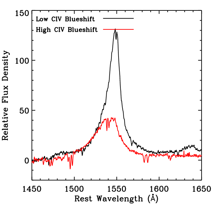
As we are more interested in the emission line properties but not the continuum of the quasar spectra, we create 2 composite spectra based on the rest-frame spectra of the two subsamples using the arithmetic mean instead of the geometric mean at each wavelength pixel. After subtracting the best-fitting pseudo-continuum from the stacked spectra, we investigate their CIV emission line profiles. As shown in Fig. 11, the blue wings are similar, while the red wing of the CIV line profile with larger blueshift is lower. It appears that the shift of the CIV emission line is not due to the blueshift of the whole profile but to the suppression of the red wing.
Richards et al. 2002 suggested that the CIV blueshifts were related to the quasar orientation, either external or internal. In a spherically symmetric cloud model (Elvis 2000; Richards et al. 2002), assuming the outflowing clouds are isotropically distributed, subsample I may represent a more face-on configuration of the accretion disk and subsample II represents a more edge-on configuration (Richards et al. 2002; Leighly 2004; Coatman et al. 2017; Coatman et al. 2016). The obscuration of the optical-thick disk in subsample II would reduce the flux of the red wing of CIV. While for a disk wind-type model (Murray & Chiang 1998), the blueshift and shape could be caused by both the orientation and a change in the opening angle of the disk wind.
However, Leighly 2004 and Richards et al. 2011 hinted that the CIV blueshifts are not likely due to the external orientation. Leighly 2004 mentioned that the blueshifted high-ionization lines may come from a wind that is moving toward us, with the receding side obscured by the optically thick accretion disk. Moreover, some studies suggested that the blueshift implied the contribution from the outflowing wind component (Richards et al. 2011; Bachev et al. 2004; Marziani et al. 2010; Vietri et al. 2018; Marziani et al. 2019).
In that way, the differences of the CIV properties between subsamples I and II are due to differences in the accretion disk wind, where the relative contribution of the wind component to the disk contribution in subsample II is larger. Furthermore, the difference of the disk wind is probably due to the difference of the spectral energy distribution, ultimately determined by the intrinsic quasar properties, such as the Eddington ratio (Richards et al. 2011; Sulentic et al. 2017; Vietri et al. 2018; Sun et al. 2018; Marziani et al. 2019).
On the other hand, we compared the REW[OIII] distribution of the two subsamples. We find that depending on REW or Å(Vietri et al. 2018), subsample I can be divided in 6 [OIII] and 3 weak [OIII] quasars; while subsample II contains 1 [OIII] quasar and 8 weak [OIII] quasars. The higher ratio of [OIII] quasars in subsample I with lower blueshifts suggests that the [OIII] quasars seem to exhibit lower blueshifts than the weak [OIII] quasars. This is qualitatively consistent with the result found in Vietri et al. 2018, where among 18 quasars with and erg s-1, the 6 [OIII] quasars show lower blueshifts than the other 12 weak [OIII] quasars.
Shen & Ho 2014 suggested that the dispersion of the FWHMHβ at fixed in the optical EV1 plane is largely an orientation effect and found no tendency of the REW[OIII] values with FWHMHβ at fixed . That indicates that the REW[OIII] distribution can not be solely explained by the orientation effect.
Since the 18 quasars of our sample exhibit values ranging from 0 to 0.47, as shown in Fig. 9, it is reasonable to assume them as quasars with almost fixed and to take the FWHMHβ as an orientation indicator. No significant correlations between FWHMHβ and the CIV blueshifts as well as REW[OIII] are found, with () and (), respectively. It indicates that neither the CIV blueshifts nor the distribution of REW[OIII] would be likely explained by the orientation effect alone.
Though our results can not help constrain the details of the Broad Emission Line Region models, the strongly blueshifted CIV line profile suggests that it is at least partly contributed by the emission in the wind. The possibility of an orientation effect can not be neglected, but the orientation effect alone is unlikely to explain either the CIV blueshift or the REW[OIII] distribution. It is possible that they are caused by the combination of the orientation effect and the intrinsic quasar properties, such as the Eddington ratio.
IV.5. Is the CIV blueshift driven by the Eddington Ratio?
As shown in Fig. 12, adopting estimated from the H-based BH masses, all the quasars in our sample are accreting at and cover a considerable range of blueshifts. It suggests that not all quasars with high Eddington ratios show large blueshifts. This is consistent with previous works (Baskin & Laor 2005; Coatman et al. 2016; Sun et al. 2018), where quasars with large CIV blueshifts tend to accrete at around Eddington limits, while the converse is not true.
The Eddington ratio is thought to be the underlying driver behind the MS (Boroson & Green 1992; Sulentic et al. 2000; Marziani et al. 2001; Bachev et al. 2004; Marziani et al. 2010; Shen & Ho 2014; Sulentic et al. 2017; Marziani et al. 2019). As the value increases, the radiation pressure plays an increasingly important role in accelerating clouds which could produce blueshifted CIV profile (Marziani et al. 2010). Previous studies found that there is a correlation between the CIV line blueshifts and the values (Marziani et al. 2010; Coatman et al. 2016; Sun et al. 2018; Vietri et al. 2018).
No similar correlation between the CIV blueshifts and is seen in our sample, with () . The median of the quasars in subsample I is , while that of the quasars in subsample II is . The scatter is estimated as the inner 50 percentile of the distribution. From the difference of the median , it seems that the quasars of subsample I accrete at higher Eddington ratio than the quasars of subsample II. However, this may not be representative of the intrinsic relationship, as both the errors of ( dex) and the scatters of the median are large compared to the difference of the median between subsample I and II. If the values are estimated from the CIV-based BH masses, as shown in red, an anti-correlation between the CIV line blueshifts and the is shown, with (). This anti-correlation is mainly due to the positive correlation between the CIV line blueshifts and the CIV-based BH masses, as shown in Section III.2.
In the optical EV1 plane, the average value increases as the increases (Shen & Ho 2014; Marziani et al. 2019). Our sample including only the Pop. A1 and Pop. B quasars with covers the left part in the optical EV1 plane. Thus we argue that the inconsistent correlation between the CIV blueshifts and in our sample is mainly due to the limited sample size and the range of the , which should be verified with a larger sample in the future.

V. CONCLUSION
Using a luminous quasar sample ( erg s-1) with observed-frame optical and NIR spectroscopy, we have investigated the reliability of estimating BH masses based on the CIV emission line and the possible corrections based on the CIV blueshift and asymmetry. We also study the CIV emission line properties, in terms of the blueshift and possible physical mechanisms therein. The conclusions are summarized as follows:
1. The logarithm of the CIV-to-H BH mass ratios are between dex and dex, with a median value as 0.110 dex and a scatter as 0.647 dex. 63% quasars in our sample show within the range of 0.4 dex. It suggests that the CIV-based BH mass estimates still need to be corrected to better match the H-based BH masses.
2. The logarithm of the CIV-to-H BH mass ratios correlate with the CIV FWHMs, the CIV blueshifts and the asymmetries. Corrections using the CIV blueshift and the asymmetry reduce the scatter of the logarithm of the mass ratio by 0.2 dex and 0.04 dex, respectively. Excluding the target with the largest CIV-to-H mass difference, the scatter is reduced by dex after the correction using the CIV asymmetry.
3. The Baldwin effect between REWCIV and is not significant in our sample, likely due to the limited luminosity range of our sample. The moderate anti-correlation between REWCIV and the CIV blueshifts is seen. No similar anti-correlation between REWCIV and (the modified Baldwin effect) is seen, which may be mainly due to the narrow range of of our sample.
4.With limited number of quasars, we find that in subsample I with positive CIV blueshifts1000 km s-1 among the 8 quasars in the FIRST footprint, 2 quasars are radio-detected including 1 radio-loud quasar with and 1 radio-quiet quasar with , while in subsample II among the 8 quasars in the FIRST footprint, 1 quasar is radio-detected in the FIRST with . Whether it suggests that a higher blueshift sample is more radio quiet, still needs to be verified using a larger quasar sample in the future.
5. Among the 19 quasars, 6 quasars are the Pop. A1 and 12 are the Pop. B quasars. 50 of the Pop. B quasars exhibit the CIV blueshifts larger than 1000 km s-1, extending the detection of significant CIV blueshifts in luminous Pop. B quasars.
6. After comparing the CIV emission line profiles of the composite spectra of subsamples I and II, we find a lack of flux in the red wing for the CIV composite emission line of subsample II with larger blueshifts. The ratio of [OIII] quasars with REW Å in subsample I is higher by 55.6 than that in subsample II, suggesting that the [OIII] quasars seem to exhibit lower blueshifts than the weak [OIII] quasars with REW Å.
7. Considering that our sample mainly covers a narrow range of , we take the FWHMHβ as an indicator of the orientation. No significant correlation between FWHMHβ and the CIV blueshifts or REW[OIII] is found, indicating that the orientation effect alone can not explain either the difference of the CIV profile for quasars with different blueshifts or the distribution of REW[OIII]. It is more likely that they are caused by the orientation effect and the intrinsic quasar properties, such as the Eddington ratio.
8. Quasars in our sample accrete at high Eddington ratios with and show a wide range of CIV blueshifts, with 18/19 of the quasars showing CIV blueshifts (with the median value of 1126 km s-1) and 14/19 of the quasars showing CIV blueshifts larger than 500 km s-1.
| Name (SDSS) | S/N | Note | |
|---|---|---|---|
| (1) | (2) | (3) | (4) |
| J011521.20+152453.3 | 2 | 23.61 | DR7, highest S/N |
| J014214.75+002324.2 | 1 | 20.37 | DR7 |
| J015741.57-010629.6 | 3 | 19.22 | DR7 |
| 22.61 | DR7, highest S/N | ||
| J025021.76-075749.9 | 2 | 20.62 | DR7, highest S/N |
| J025905.63+001121.9 | 6 | 23.79 | DR7 |
| 37.03 | DR7, highest S/N | ||
| J030341.04-002321.9 | 4 | 25.87 | DR7 |
| 27.99 | DR7, highest S/N | ||
| J030449.85-000813.4 | 7 | 29.62 | DR7, highest S/N |
| J075303.34+423130.8 | 4 | 32.94 | DR7 |
| 40.69 | DR7, highest S/N | ||
| J080430.56+542041.1 | 2 | 22.62 | DR7, highest S/N |
| J080819.69+373047.3 | 4 | 12.55 | DR7 |
| 19.35 | DR7, highest S/N | ||
| J080956.02+502000.9 | 3 | 18.8 | DR7 |
| 27.56 | DR7, highest S/N | ||
| J081855.77+095848.0 | 1 | 20.67 | DR7 |
| J090033.50+421547.0 | 2 | 40.85 | DR7 |
| 47.48 | DR7, highest S/N | ||
| J094202.04+042244.5 | 2 | 28.96 | DR7 |
| 41.07 | DR7, highest S/N | ||
| J115954.33+201921.1 | 1 | 39.94 | DR7 |
| J173352.23+540030.4 | 4 | 35.5 | DR7 |
| 36.11 | DR7, highest S/N | ||
| J213023.61+122252.0 | 1 | 21.24 | DR7 |
| J224956.08+000218.0 | 2 | 14.56 | DR7 |
| 24.95 | DR7, highest S/N | ||
| J230301.45-093930.7 | 1 | 26.33 | DR7 |
Note. — Col.(1) Name of the quasars. Col.(2) Number of spectra for this quasar in the SDSS DR14 database. Col.(3) Average S/N per pixel of this spectrum. Col.(4)‘DR7’ means that the row refers to the information of the spectrum used in the SDSS DR7 catalog (Shen et al. 2011). ‘DR7’ means that the row refers to the information of the spectrum with the highest S/N per pixel after the SDSS DR7.
| Name (SDSS) | — REW0 — FWHM0 | — REW1 — FWHM1 | — REW2 — FWHM2 | BC indexes | — REW — FWHM | Model |
|---|---|---|---|---|---|---|
| (km s-1 — Å— km s-1) | (km s-1 — Å— km s-1) | (km s-1 — Å— km s-1) | (km s-1 — Å— km s-1) | |||
| (1) | (2) | (3) | (4) | (5) | (6) | (7) |
| J011521.20+152453.3 | / 11 / 6362 | / 9 / 4227 | / 7 / 22831 | 0,1,2 | / 27 / 6483 | A |
| J014214.75+002324.2 | / 7 / 3261 | / 16 / 11486 | / 0 / 6496 | 0,1,2 | / 24 / 4730 | A |
| J015741.57-010629.6 | / 26 / 12906 | / 19 / 4952 | / 4 / 1600 | 0,1 | / 45 / 6489 | B |
| J025021.76-075749.9 | / 3 / 2722 | / 15 / 8950 | / 1 / 853 | 0,1 | / 18 / 6983 | B |
| J025905.63+001121.9 | / 28 / 13567 | / 26 / 4486 | / 10 / 1600 | 0,1 | / 55 / 5562 | B |
| J030341.04-002321.9 | / 3 / 2310 | / 17 / 6233 | / 14 / 15617 | 0,1,2 | / 34 / 6383 | A |
| J030449.85-000813.4 | / 13 / 11092 | / 8 / 2563 | / 4 / 1285 | 0,1 | / 21 / 3261 | B |
| J075303.34+423130.8 | / 18 / 8671 | / 9 / 2114 | / 0 / 1600 | 0,1 | / 27 / 2903 | B |
| J080430.56+542041.1 | / 15 / 9893 | / 5 / 15309 | / 10 / 4612 | 0,1,2 | / 30 / 7041 | A |
| J080819.69+373047.3 | / 20 / 5937 | / 11 / 21070 | / 0 / 984 | 0,1 | / 31 / 6714 | B |
| J080956.02+502000.9 | / 9 / 2362 | / 17 / 12375 | / 17 / 4872 | 0,1,2 | / 43 / 4016 | A |
| J081855.77+095848.0 | / 13 / 14787 | / 11 / 5206 | / 0 / 5631 | 0,1,2 | / 25 / 6860 | A |
| J090033.50+421547.0 | / 11 / 3319 | / 26 / 11593 | / 1 / 1600 | 0,1 | / 36 / 4888 | B |
| J094202.04+042244.5 | / 16 / 4595 | / 7 / 1761 | / 17 / 13385 | 0,1,2 | / 40 / 3356 | A |
| J115954.33+201921.1 | / 7 / 27583 | / 12 / 6504 | / 0 / 1410 | 0,1,2 | / 19 / 7525 | A |
| J173352.23+540030.4 | / 5 / 4095 | / 9 / 12457 | / 2 / 2165 | 0,1,2 | / 16 / 5273 | A |
| J213023.61+122252.0 | / 10 / 29638 | / 17 / 5852 | / 8 / 1647 | 0,1,2 | / 35 / 2474 | A |
| J224956.08+000218.0 | / 22 / 4067 | / 18 / 2070 | / 24 / 14643 | 0,1,2 | / 65 / 3160 | A |
| J230301.45-093930.7 | / 4 / 4175 | / 0 / 4973 | / 15 / 13763 | 0,1,2 | / 19 / 9453 | A |
Note. — Col.(1) Name of the quasars. The name in bold refer to the quasars, the [OIII] doublets of which were fitted with two pairs of Gaussians. Col.(2) CIV emission-line velocity shift with respect to [OIII] 5007, REW and FWHM of the 1st Gaussian for the CIV line fitting. Col.(3) , REW and FWHM of the 2nd Gaussian for the CIV line fitting. Col.(4) , REW and FWHM of the 3rd Gaussian for the CIV line fitting. Col.(5) The indexes of Gaussians for the CIV BC. Col.(6) , REW and FWHM of the CIV BC. Col.(7) Fitting model of the CIV emission line. In Model A, 3 Gaussians are fitted to the CIV BC and the contribution of the CIV NC is not considered, while in Model B, 2/1 Gaussians are fitted to the CIV BC/NC.
| Name (SDSS) | FWHMCIV | REWCIV | — | loudness — R | DR7 T — DR7 T — NIR T | |||
|---|---|---|---|---|---|---|---|---|
| (erg s-1) | (km s-1) | () | (Å) | (km s-1 — km s-1) | flag — | |||
| (1) | (2) | (3) | (4) | (5) | (6) | (7) | (8) | (9) |
| J011521.20+152453.3 | 3.443 | 46.95 | 6483 200 | 9.85 0.03 | 27 1 | 2433 352 / 2678 277 | -1 / -1 | 071205/ 071205 / 111022 |
| J014214.75+002324.2 | 3.379 | 47.01 | 4730 227 | 9.61 0.04 | 24 1 | 962 105 / 965 100 | 0 / -1 | 000901/ 000901 / 111021 |
| J015741.57-010629.6 | 3.572 | 46.99 | 6489 149 | 9.87 0.02 | 45 1 | 1918 75 / 1590 61 | 0 / -1 | 001123/ 100910 / 111021 |
| J025021.76-075749.9 | 3.337 | 47.03 | 6983 992 | 9.95 0.12 | 18 1 | 140 776 / 1233 233 | 0 / -1 | 001223/ 001223 / 111021 |
| J025905.63+001121.9 | 3.373 | 47.16 | 5562 116 | 9.83 0.02 | 55 1 | 957 54 / 847 37 | 1 / 5.5 | 001223/ 101007 / 111021 |
| J030341.04-002321.9 | 3.233 | 47.16 | 6383 386 | 9.95 0.05 | 34 1 | 511 261 / 946 217 | 0 / -1 | 000930/ 011023 / 111022 |
| J030449.85-000813.4 | 3.287 | 47.38 | 3261 892 | 9.48 0.19 | 21 1 | 421 137 / 506 106 | 0 / -1 | 000930/ 000930 / 111020 |
| J075303.34+423130.8 | 3.590 | 47.22 | 2903 731 | 9.29 0.15 | 27 1 | 22 93 / 117 42 | 1 / 2645.3 | 000930/ 091213 / 111020 |
| J080430.56+542041.1 | 3.759 | 47.10 | 7041 253 | 10.00 0.031 | 30 1 | 1258 155 / 1570 102 | 0 / -1 | 050114/ 050114 / 111022 |
| J080819.69+373047.3 | 3.480 | 46.85 | 6714 341 | 9.82 0.04 | 31 1 | 1755 120 / 1150 149 | 0 / -1 | 011210/ 100312 / 111021 |
| J080956.02+502000.9 | 3.281 | 47.03 | 4016 73 | 9.48 0.02 | 43 1 | 147 176 / 296 163 | 0 / -1 | 040326/ 101117 / 111022 |
| J081855.77+095848.0 | 3.700 | 47.09 | 6860 479 | 9.97 0.06 | 25 1 | 1954 282 / 1967 168 | 0 / -1 | 070218/ 070218 / 111021/22 |
| J090033.50+421547.0 | 3.290 | 47.49 | 4888 522 | 9.89 0.08 | 36 1 | -360 205 / -282 196 | 1 / 2.1 | 020120/ 120226 / 120415 |
| J094202.04+042244.5 | 3.276 | 47.37 | 3356 51 | 9.50 0.01 | 40 | 372 111 / 788 110 | 0 / -1 | 011223/ 010411 / 120415 |
| J115954.33+201921.1 | 3.426 | 47.40 | 7525 310 | 10.21 0.041 | 19 | 1447 533 / 1126 56 | 0 / -1 | 080109/ 080109 / 120416 |
| J173352.23+540030.4 | 3.432 | 47.45 | 5273 136 | 9.93 0.02 | 16 1 | 254 712 / 1355 703 | 1 / 14.0 | 000929/ 010331 / 120415 |
| J213023.61+122252.0 | 3.272 | 47.10 | 2474 77 | 9.09 0.03 | 35 1 | 16 31 / 46 36 | -1 / -1 | 020705/ 020705 / 111021 |
| J224956.08+000218.0 | 3.311 | 46.90 | 3160 42 | 9.20 0.01 | 65 1 | 226 35 / 490 25 | 0 / -1 | 021112/ 101002 / 111022 |
| J230301.45-093930.7 | 3.492 | 47.27 | 9453 453 | 10.34 0.041 | 19 1 | 1685 540 / 1923 392 | 0 / -1 | 011215/ 011215 / 111020 |
Note. — Col.(1) Name of the quasars. Col.(2) Redshift measured from the H and the [OIII] doublets of the near-IR spectra. Col.(3) Continuum luminosity at 1350 Å. Col.(4) FWHM of the CIV BC. Col.(5) CIV line-based BH masses estimated using the calibration from Vestergaard & Peterson 2006. The uncertainties quoted are only from statistical errors and not including the intrinsic uncertainties of the SE virial BH mass estimates as dex (Vestergaard 2002). Col.(6) REW of the CIV emission line. Col.(7) CIV emission-line velocity shifts and with respect to [OIII] 5007. Col.(8) FIRST radio flag: -1 = not in FIRST footprint; 0 = FIRST undetected; 1 = core dominant. Radio loudness R = . Col.(9) Date when the SDSS DR7 / SDSS DR7 / Near-IR spectroscopy were taken, eg. 071110 referring to Nov. 10, 2007.
| c | ||||
|---|---|---|---|---|
| (1) | (2) | (3) | (4) | (5) |
| 0.66 | 0.53 | 2.0 | 0.110 | 0.647 |
| 8.01 0.26 | 0.53 | 0 | 0.025 | 0.360 |
| 2.26 0.38 | 0 | 2.0 | 0.006 | 0.432 |
| Variable | ||
|---|---|---|
| (1) | (2) | (3) |
| 0.31 | 0.19 | |
| 0.04 | 0.86 | |
| 0.20 | 0.42 | |
| 0.67 | ||
| 0.09 | ||
| 0.98 | ||
| CIV Blueshift | 0.54 | 0.02 |
| CIV Asymmetry ASCIV |
Note. — Col.(2) The Spearman rank correlation coefficient . Col.(3) The significance of deviated from the null hypothesis.
We thank the anonymous referee for his/her helpful comments that improved the paper. We thank the supports by the Ministry of Science and Technology of China under grant 2016YFA0400703, the NSFC grants No.11373008 and 11533001, and the National Key Basic Research Program of China 2014CB845700. This work made use of the facilities of the Center for High Performance Computing at Shanghai Astronomical Observatory, Chinese Academy of Sciences. This research uses data obtained through the Telescope Access Program (TAP), which is funded by the National Astronomical Observatories, Chinese Academy of Sciences, and the Special Fund for Astronomy from the Ministry of Finance. Observations obtained with the Hale Telescope at Palomar Observatory were obtained as part of an agreement between the National Astronomical Observatories, Chinese Academy of Sciences, and the California Institute of Technology. The LBT is an international collabofn among institutions in the United States, Italy and Germany. LBT Corporation partners are: The University of Arizona on behalf of the Arizona university system; Istituto Nazionale di Astrofisica, Italy; LBT Beteiligungsgesellschaft, Germany, representing the Max-Planck Society, the Astrophysical Institute Potsdam, and Heidelberg University; The Ohio State University, and The Research Corporation, on behalf of The University of Notre Dame, University of Minnesota and University of Virginia. Funding for the SDSS and SDSS-II has been provided by the Alfred P. Sloan Foundation, the Participating Institutions, the National Science Foundation, the U.S. Department of Energy, the National Aeronautics and Space Administration, the Japanese Monbukagakusho, the Max Planck Society, and the Higher Education Funding Council for England. The SDSS Web Site is http://www.sdss.org/. The SDSS is managed by the Astrophysical Research Consortium for the Participating Institutions. The Participating Institutions are the American Museum of Natural History, Astrophysical Institute Potsdam, University of Basel, University of Cambridge, Case Western Reserve University, University of Chicago, Drexel University, Fermilab, the Institute for Advanced Study, the Japan Participation Group, Johns Hopkins University, the Joint Institute for Nuclear Astrophysics, the Kavli Institute for Particle Astrophysics and Cosmology, the Korean Scientist Group, the Chinese Academy of Sciences (LAMOST), Los Alamos National Laboratory, the Max-Planck-Institute for Astronomy (MPIA), the Max- Planck-Institute for Astrophysics (MPA), New Mexico State University, Ohio State University, University of Pittsburgh, University of Portsmouth, Princeton University, the United States Naval Observatory, and the University of Washington.
References
- Akaike (1974) Akaike, H. 1974, IEEE Transactions on Automatic Control, 19, 716
- Akritas & Bershady (1996) Akritas, M. G., & Bershady, M. A. 1996, ApJ, 470, 706
- Allen et al. (2013) Allen, J. T., Hewett, P. C., Richardson, C. T., Ferland, G. J., & Baldwin, J. A. 2013, MNRAS, 430, 3510
- Assef et al. (2011) Assef, R. J., Denney, K. D., Kochanek, C. S., et al. 2011, ApJ, 742, 93
- Bachev et al. (2004) Bachev, R., Marziani, P., Sulentic, J. W., et al. 2004, ApJ, 617, 171
- Baldwin (1977) Baldwin, J. A. 1977, ApJ, 214, 679
- Barth et al. (2015) Barth, A. J., Bennert, V. N., Canalizo, G., et al. 2015, ApJS, 217, 26
- Baskin & Laor (2005) Baskin, A., & Laor, A. 2005, MNRAS, 356, 1029
- Becker et al. (2009) Becker, G. D., Rauch, M., & Sargent, W. L. W. 2009, ApJ, 698, 1010
- Bentz et al. (2009) Bentz, M. C., Peterson, B. M., Netzer, H., Pogge, R. W., & Vestergaard, M. 2009, ApJ, 697, 160
- Bentz et al. (2013) Bentz, M. C., Denney, K. D., Grier, C. J., et al. 2013, ApJ, 767, 149
- Bian et al. (2010) Bian, F., Fan, X., Bechtold, J., et al. 2010, ApJ, 725, 1877
- Boroson & Green (1992) Boroson, T. A., & Green, R. F. 1992, ApJS, 80, 109
- Cardelli et al. (1989) Cardelli, J. A., Clayton, G. C., & Mathis, J. S. 1989, ApJ, 345, 245
- Coatman et al. (2016) Coatman, L., Hewett, P. C., Banerji, M., & Richards, G. T. 2016, MNRAS, 461, 647
- Coatman et al. (2017) Coatman, L., Hewett, P. C., Banerji, M., et al. 2017, MNRAS, 465, 2120
- Coffey et al. (2019) Coffey, D., Salvato, M., Merloni, A., et al. 2019, A&A, 625, A123
- Cushing et al. (2004) Cushing, M. C., Vacca, W. D., & Rayner, J. T. 2004, PASP, 116, 362
- Denney (2012) Denney, K. D. 2012, ApJ, 759, 44
- Denney et al. (2010) Denney, K. D., Peterson, B. M., Pogge, R. W., et al. 2010, ApJ, 721, 715
- Du et al. (2014) Du, P., Hu, C., Lu, K.-X., et al. 2014, ApJ, 782, 45
- Elvis (2000) Elvis, M. 2000, ApJ, 545, 63
- Feibelman (1983) Feibelman, W. A. 1983, A&A, 122, 335
- Ferrarese & Merritt (2000) Ferrarese, L., & Merritt, D. 2000, ApJ, 539, L9
- Gaskell (1982) Gaskell, C. M. 1982, ApJ, 263, 79
- Ge et al. (2016) Ge, X., Bian, W.-H., Jiang, X.-L., Liu, W.-S., & Wang, X.-F. 2016, MNRAS, 462, 966
- Ge et al. (2019) Ge, X., Zhao, B.-X., Bian, W.-H., & Frederick, G. R. 2019, AJ, 157, 148
- Gebhardt et al. (2000) Gebhardt, K., Bender, R., Bower, G., et al. 2000, ApJ, 539, L13
- Graham et al. (2011) Graham, A. W., Onken, C. A., Athanassoula, E., & Combes, F. 2011, MNRAS, 412, 2211
- Greene & Ho (2005) Greene, J. E., & Ho, L. C. 2005, ApJ, 630, 122
- Greene et al. (2010) Greene, J. E., Peng, C. Y., & Ludwig, R. R. 2010, ApJ, 709, 937
- Grier et al. (2017) Grier, C. J., Trump, J. R., Shen, Y., et al. 2017, ApJ, 851, 21
- Grier et al. (2019) Grier, C. J., Shen, Y., Horne, K., et al. 2019, arXiv e-prints, arXiv:1904.03199
- Gültekin et al. (2009) Gültekin, K., Richstone, D. O., Gebhardt, K., et al. 2009, ApJ, 698, 198
- Herter et al. (2008) Herter, T. L., Henderson, C. P., Wilson, J. C., et al. 2008, in Society of Photo-Optical Instrumentation Engineers (SPIE) Conference Series, Vol. 7014, Society of Photo-Optical Instrumentation Engineers (SPIE) Conference Series
- Hill et al. (2012) Hill, J. M., Green, R. F., Ashby, D. S., et al. 2012, in Society of Photo-Optical Instrumentation Engineers (SPIE) Conference Series, Vol. 8444, Society of Photo-Optical Instrumentation Engineers (SPIE) Conference Series
- Jiang et al. (2007) Jiang, L., Fan, X., Ivezić, Ž., et al. 2007, ApJ, 656, 680
- Kaspi et al. (2007) Kaspi, S., Brandt, W. N., Maoz, D., et al. 2007, ApJ, 659, 997
- Kaspi et al. (2005) Kaspi, S., Maoz, D., Netzer, H., et al. 2005, ApJ, 629, 61
- Kaspi et al. (2000) Kaspi, S., Smith, P. S., Netzer, H., et al. 2000, ApJ, 533, 631
- Kelly (2007) Kelly, B. C. 2007, ApJ, 665, 1489
- Konigl & Kartje (1994) Konigl, A., & Kartje, J. F. 1994, ApJ, 434, 446
- Kormendy & Ho (2013) Kormendy, J., & Ho, L. C. 2013, ARA&A, 51, 511
- Leighly (2004) Leighly, K. M. 2004, ApJ, 611, 125
- MacLeod et al. (2012) MacLeod, C. L., Ivezić, Ž., Sesar, B., et al. 2012, ApJ, 753, 106
- Marziani et al. (2001) Marziani, P., Calvani, M., & Braito, V. 2001, Mem. Soc. Astron. Italiana, 72, 41
- Marziani et al. (1996) Marziani, P., Sulentic, J. W., Dultzin-Hacyan, D., Calvani, M., & Moles, M. 1996, ApJS, 104, 37
- Marziani et al. (2010) Marziani, P., Sulentic, J. W., Negrete, C. A., et al. 2010, MNRAS, 409, 1033
- Marziani et al. (2003) Marziani, P., Zamanov, R. K., Sulentic, J. W., & Calvani, M. 2003, MNRAS, 345, 1133
- Marziani et al. (2019) Marziani, P., del Olmo, A., Martínez-Carballo, M. A., et al. 2019, A&A, 627, A88
- McGill et al. (2008) McGill, K. L., Woo, J.-H., Treu, T., & Malkan, M. A. 2008, ApJ, 673, 703
- McLure & Jarvis (2002) McLure, R. J., & Jarvis, M. J. 2002, MNRAS, 337, 109
- Mejía-Restrepo et al. (2018) Mejía-Restrepo, J. E., Trakhtenbrot, B., Lira, P., & Netzer, H. 2018, MNRAS, 478, 1929
- Murray & Chiang (1998) Murray, N., & Chiang, J. 1998, ApJ, 494, 125
- Murray et al. (1995) Murray, N., Chiang, J., Grossman, S. A., & Voit, G. M. 1995, ApJ, 451, 498
- Nelson et al. (2004) Nelson, C. H., Green, R. F., Bower, G., Gebhardt, K., & Weistrop, D. 2004, ApJ, 615, 652
- Onken et al. (2004) Onken, C. A., Ferrarese, L., Merritt, D., et al. 2004, ApJ, 615, 645
- Park et al. (2017) Park, D., Barth, A. J., Woo, J.-H., et al. 2017, ApJ, 839, 93
- Park et al. (2013) Park, D., Woo, J.-H., Denney, K. D., & Shin, J. 2013, ApJ, 770, 87
- Peterson (1993) Peterson, B. M. 1993, PASP, 105, 247
- Peterson et al. (2004) Peterson, B. M., Ferrarese, L., Gilbert, K. M., et al. 2004, ApJ, 613, 682
- Proga et al. (2000) Proga, D., Stone, J. M., & Kallman, T. R. 2000, ApJ, 543, 686
- Richards et al. (2002) Richards, G. T., Vanden Berk, D. E., Reichard, T. A., et al. 2002, AJ, 124, 1
- Richards et al. (2006) Richards, G. T., Lacy, M., Storrie-Lombardi, L. J., et al. 2006, ApJS, 166, 470
- Richards et al. (2011) Richards, G. T., Kruczek, N. E., Gallagher, S. C., et al. 2011, AJ, 141, 167
- Runnoe et al. (2013) Runnoe, J. C., Brotherton, M. S., Shang, Z., & DiPompeo, M. A. 2013, MNRAS, arXiv:1306.3521
- Schlegel et al. (1998) Schlegel, D. J., Finkbeiner, D. P., & Davis, M. 1998, ApJ, 500, 525
- Schneider et al. (2010) Schneider, D. P., Richards, G. T., Hall, P. B., et al. 2010, AJ, 139, 2360
- Schulze et al. (2018) Schulze, A., Silverman, J. D., Kashino, D., et al. 2018, ApJS, 239, 22
- Shemmer & Lieber (2015) Shemmer, O., & Lieber, S. 2015, ApJ, 805, 124
- Shen (2013) Shen, Y. 2013, Bulletin of the Astronomical Society of India, 41, 61
- Shen et al. (2008) Shen, Y., Greene, J. E., Strauss, M. A., Richards, G. T., & Schneider, D. P. 2008, ApJ, 680, 169
- Shen & Ho (2014) Shen, Y., & Ho, L. C. 2014, Nature, 513, 210
- Shen & Liu (2012) Shen, Y., & Liu, X. 2012, ApJ, 753, 125
- Shen et al. (2011) Shen, Y., Richards, G. T., Strauss, M. A., et al. 2011, ApJS, 194, 45
- Shen et al. (2015) Shen, Y., Brandt, W. N., Dawson, K. S., et al. 2015, ApJS, 216, 4
- Shen et al. (2019) Shen, Y., Grier, C. J., Horne, K., et al. 2019, ApJ, 883, L14
- Sulentic et al. (2007) Sulentic, J. W., Bachev, R., Marziani, P., Negrete, C. A., & Dultzin, D. 2007, ApJ, 666, 757
- Sulentic et al. (2000) Sulentic, J. W., Marziani, P., & Dultzin-Hacyan, D. 2000, ARA&A, 38, 521
- Sulentic et al. (2017) Sulentic, J. W., del Olmo, A., Marziani, P., et al. 2017, A&A, 608, A122
- Sun et al. (2018) Sun, M., Xue, Y., Richards, G. T., et al. 2018, ApJ, 854, 128
- Trakhtenbrot & Netzer (2012) Trakhtenbrot, B., & Netzer, H. 2012, MNRAS, 427, 3081
- Tremaine et al. (2002) Tremaine, S., Gebhardt, K., Bender, R., et al. 2002, ApJ, 574, 740
- Vanden Berk et al. (2001) Vanden Berk, D. E., Richards, G. T., Bauer, A., et al. 2001, AJ, 122, 549
- Vestergaard (2002) Vestergaard, M. 2002, ApJ, 571, 733
- Vestergaard & Osmer (2009) Vestergaard, M., & Osmer, P. S. 2009, ApJ, 699, 800
- Vestergaard & Peterson (2006) Vestergaard, M., & Peterson, B. M. 2006, ApJ, 641, 689
- Vietri et al. (2018) Vietri, G., Piconcelli, E., Bischetti, M., et al. 2018, A&A, 617, A81
- Wilhite et al. (2007) Wilhite, B. C., Brunner, R. J., Schneider, D. P., & Vanden Berk, D. E. 2007, ApJ, 669, 791
- Zuo et al. (2015) Zuo, W., Wu, X.-B., Fan, X., et al. 2015, ApJ, 799, 189
- Zuo et al. (2012) Zuo, W., Wu, X.-B., Liu, Y.-Q., & Jiao, C.-L. 2012, ApJ, 758, 104
In Model A, we fit 3 Gaussians for the BC of CIV, 1 Gaussian for the BC of HeII and 1 Gaussian for the BC of OIII . In model B, we fit 2/1 Gaussians for the BC/NC of CIV, 1/1 Gaussian for the BC/NC of HeII and 1/1 Gaussian for the BC/NC of OIII]. The NC of the three lines are tied together and fitted with an upper FWHM limit as 1600 km s-1. We also compare them with Model C, where the only difference from Model A is that the number of Gaussians used to fit the CIV BC in Model C is 2 instead of 3.
Fig. 13 and Fig. 14 present the spectra fitting results of Model A and Model B in the wavelength range of 1500-1700 Å for the 19 quasars, respectively. The reduced of the spectral fitting of the CIV emission line using Model A, B and C are listed in Table 6, with the median values as 1.070.25, 1.060.27 and 1.160.34, respectively. Model A yields the smallest for 68.4% quasars, though considering the scatter, the values of the three models are similar.
However, after visual inspections, we find that for most quasars the 3-Gaussian models (Model A and B) for the CIV line reproduces the CIV line profile better than the 2-Gaussian Model (Model C). It is reasonable as there are more adjustable parameters to maximize the consistence between the model fitting and the observed data. For some quasars, such as and , the fitting results from Model B show a weird NC due to the narrow spikes in the noisy regions of the spectra.
If the candidate model selected from the visual inspection (as listed in Col. (7) of Table 6) is different from the the best model according to the comparison (as listed in Col. (6)), we adopt the candidate model from the visual inspection. If both Model A and Model B are listed in Col. (6) and Col. (7), we adopt the results from the Model A, which is supported by the Akaike information criterion (AIC) comparison, as listed in Col. (5).
To determine the best model for the data, we derive the AIC values of Model A and Model B for each object. The optimal choice is the one with the smaller AIC value. The AIC is calculated as
| (8) |
where is the set of model parameters, k is the number of the independently adjusted parameters in the candidate model, is the likelihood of the candidate model giving the data when evaluated at the maximum likelihood estimate of (Akaike 1974). The derived AIC values from Model A and Model B are listed in Table 6, showing that Model A is better to approximate the data than Model B.
In all, for 7 quasars (, , , , , and ), small fitting residuals around the CIV line are seen in the results from Model A but not shown in the results from Model B. Therefore, for these 7 quasars we use the results from Model B and for the other 12 quasars we adopt the results from Model A.


| Name (SDSS) | AICA-AICB | Visual | Final | ||||
|---|---|---|---|---|---|---|---|
| A | B | C | comparison | inspection | |||
| (1) | (2) | (3) | (4) | (5) | (6) | (7) | (8) |
| J011521.20+152453.3 | 1.29 | 1.30 | 1.34 | -4.001 | A | A | A |
| J014214.75+002324.2 | 1.21 | 1.20 | 1.24 | -4.004 | B | A | A |
| J015741.57-010629.6 | 0.96 | 0.88 | 1.08 | -3.998 | B | B | B |
| J025021.76-075749.9 | 0.96 | 0.96 | 0.98 | -3.999 | AB | B | B |
| J025905.63+001121.9 | 1.02 | 1.00 | 2.18 | -4.000 | B | AB | B |
| J030341.04-002321.9 | 0.97 | 1.00 | 1.07 | -4.001 | A | A | A |
| J030449.85-000813.4 | 0.90 | 0.93 | 1.00 | -4.000 | A | B | B |
| J075303.34+423130.8 | 1.97 | 1.88 | 1.89 | -3.998 | B | AB | B |
| J080430.56+542041.1 | 1.16 | 1.18 | 1.16 | -4.003 | A | A | A |
| J080819.69+373047.3 | 1.09 | 0.89 | 0.87 | -3.984 | B | B | B |
| J080956.02+502000.9 | 1.01 | 1.06 | 1.23 | -4.001 | A | A | A |
| J081855.77+095848.0 | 1.17 | 1.19 | 1.16 | -3.998 | A | A | A |
| J090033.50+421547.0 | 1.07 | 1.11 | 1.12 | -4.001 | A | B | B |
| J094202.04+042244.5 | 1.00 | 1.00 | 1.39 | -4.000 | AB | AB | A |
| J115954.33+201921.1 | 1.11 | 1.10 | 1.18 | -3.997 | B | A | A |
| J173352.23+540030.4 | 0.85 | 0.85 | 0.90 | -4.000 | AB | AB | A |
| J213023.61+122252.0 | 1.22 | 1.24 | 1.28 | -4.001 | A | AB | A |
| J224956.08+000218.0 | 1.35 | 1.39 | 1.92 | -4.001 | A | A | A |
| J230301.45-093930.7 | 0.89 | 0.90 | 0.90 | -4.002 | A | A | A |
Note. — Col.(1) Name of the quasars. Col.(2) Reduced of the spectral fitting to the CIV line complex using Model A. Col.(3) Reduced of the spectral fitting to the CIV line complex using Model B. Col.(4) Reduced of the spectral fitting to the CIV line complex using Model C. Col.(5) Difference of the AIC values between Model A and Model B. Col.(6) The preferred model with the lower reduced between Model A and Model B. Col.(7) The preferred model from the visual inspection between Model A and Model B. Col.(8) The final adopted model from the combination of the results from Col.(5-7).