Controller tuning in power systems using singular value optimization AM (amer.mesanovic@siemens.com), RF (rolf.findeisen@ovgu.de) are with the Laboratory for Systems Theory and Automatic Control, Otto-von- Guericke-University Magdeburg, Germany, AM is also with the Siemens AG, Munich, UM (ulrich.muenz@siemens.com) is with Siemens Corp., Princeton. This work has been partially funded by the German Federal Ministry of Education and Research (BMBF) under Grant number 01S18066B in the frame of the AlgoRes project.
Abstract
As the share of renewable generation in large power systems continues to increase, the operation of power systems becomes increasingly challenging. The constantly shifting mix of renewable and conventional generation leads to largely changing dynamics, increasing the risk of blackouts. We propose to retune the parameters of the already present controllers in the power systems to account for the seemingly changing operating conditions. To this end, we present an approach for fast and computationally efficient tuning of parameters of structured controllers. The goal of the tuning is to shift system poles to a specified region in the complex plane, e.g. for stabilization or oscillation damping. The approach exploits singular value optimization in the frequency domain, which enables scaling to large systems and is not limited to power systems. The efficiency of the approach is shown on three systems of increasing size with multiple initial parameterizations.
keywords
Pole placement, singular value, optimization, stabilization, linear matrix inequalities1 Introduction
The rising share of renewable generation in power systems leads to increased volatility and uncertainty in their operation. Depending on weather conditions, the power generation of renewables in the power grid varies temporally, as well as geographically. Furthermore, in the case of challenging weather conditions, conventional generation, e.g. thermal power plants, needs to compensate for the reduced renewable power generation. This leads to changing dynamics in power systems, such as time-varying oscillatory modes (Al Ali et al. 2014; Crivellaro et al. 2019). Doing so is challenged by the fact that existing automation systems are designed for fixed, known, dynamics (Kundur 1993) and that control systems of components are typically parameterized manually during installation, which is a time-consuming task. Not adapting the system leads to time-varying dynamics in the system, which increases the risk of a blackout. Changing the existing control system entirely to increase the stability margins is typically not possible for cost reasons and as the existing systems are trusted by operators due to decades of practical operation.
We propose to address this challenge by adapting the parameters of the existing control system to the changing conditions. To this end, we propose an iterative singular value optimization based approach, which shifts poles of linear systems to desired regions. The approach allows to tune the parameters of existing structured controllers in the system, such as PID controllers, washout filters and notch filters allowing for a nonlinear dependency on the controller parameters. Shifting poles to specific regions allows to guarantee properties such as stability, improved oscillation damping, and robustness (Scherer and Weiland 2019).
Notably in recent years, significant advances were made with respect to the characterization of the set of internally stabilizing controllers. Many extensions from the famous Youla parameterization (Youla et al. 1976), such as Bamieh et al. 2002 and Nayyar et al. 2013 have been achieved. Other approaches include quadratic invariance (Rotkowitz and Lall 2005), system level approaches (Wang et al. 2019), and closed-loop response shaping (Zheng et al. 2019). These approaches consider dynamic state- or output-feedback controllers with linear dynamic dependencies subject to various constraints on the controller parameters. A second area with fruitful results in recent years is optimization with stability constraints, Benner et al. 2018; Apkarian and Noll 2018. Approaches for pole placement, which can shift poles to specified regions in the complex plane, typically introduce a Lyapunov matrix for the synthesis procedure (Chilali and Gahinet 1996), making the approach generally less scalable. Only few approaches consider the optimization of existing controller parameters in power systems (Befekadu and Erlich 2006; Marinescu et al. 2009; Kammer and Karimi 2017). These approaches require either manual adaptation for each power system (Marinescu et al. 2009), or assume specific dependencies on the controller parameters (Befekadu and Erlich 2006; Kammer and Karimi 2017).
In contrast to existing works, we propose a method for pole placement based on singular value optimization. It is based on frequency domain considerations, and thus avoids the direct formulation of (large-scale) Lyapunov matrices, making the approach generally scalable to larger systems. Previous works of the authors consider H-infinity controller synthesis, see (Mešanović et al. 2017; Mešanović et al. 2018; Mešanović et al. 2019).
The remainder of this work is organized as follows: Section 2 derives suitable models and formulates the pole placement problem tailored towards power systems. The proposed approach is introduced in Section 3. In Section 4 the performance of the approach is underlined considering three numerical examples with multiple initial parameterizations. Finally, conclusions are provided in Section 5.
1.1 Mathematical preliminaries
We denote by the conjugate transpose of a matrix, and denote the largest singular value and largest eigenvalue, respectively, of a matrix. The notation (), and () is used to denote positive (semi)definiteness and negative (semi)definiteness of a matrix, respectively. We use to denote the imaginary unit, denotes the set of non-negative real numbers, denotes the set of complex numbers, and denotes the set of complex numbers with a positive real part.
Definition 1 (Lunze 2013)
A complex number is a pole of the transfer matrix , if at least one element of has a pole at .
We define the distance between a point and the curve , , as .
2 Controller tuning for power systems
Power systems consist of heterogeneous components, such as power plants, renewable generation, storage systems, households, and factories. For simplicity of presentation, we denote these components as prosumers, as they can either produce or consume electric power, c.f. Fig. 1. We differentiate between static and dynamic prosumers, depending on whether their internal dynamic behavior is modeled. The static and dynamic prosumers are coupled through the power grid. We outline subsequently how dynamic and static prosumers, as well as the power grid, can be modeled.
2.1 Power system models
Dynamic prosumers: Dynamic prosumers are dynamic systems with internal states, denoted with . We outline the structure of one dynamic prosumer, a power plant. Elements such as inverters or loads can be modeled as dynamics prosumers as well, however this is beyond the scope of this work. Dynamic prosumers contain tunable controller parameters , marked red in Fig. 1.
The structure of a typical power plant is shown in Fig. 2. It consists of a synchronous generator (SGi), an automatic voltage regulator and an exciter (AVRi), a governor and turbine (TGOVi), and in some cases a power system stabilizer (PSSi). AVRi controls the voltage at the power plant terminals to a reference value . To further improve the stability of a power system, power plants are sometimes equipped with a PSS. PSSs improve the system stability and increase the damping of oscillations by considering the plant frequency or power in the voltage control. TGOVi controls the generator frequency by adapting the mechanical power transfered to the synchronous generator. In practice, many different controllers are used (IEEE 2006). Elements with tunable controller parameters, i.e. AVRi, PSSi and TGOVi, are shown as functions of in Fig. 2.
Static prosumers: Static prosumers represent elements with no internal states/dynamics. They are characterized by their active power infeed and reactive power infeed , which are considered as external inputs into the model. Static prosumers, marked blue in Fig. 1, often model renewable generation and loads (Poolla et al. 2019). A subset of static prosumer infeeds is chosen as the disturbance input into the system.
Power grid: Dynamic and static prosumers are interconnected through the power grid, consisting of power lines, cables etc. The dynamic response of the power grid is typically orders of magnitude faster than the generation dynamics relevant for stability studies (Kundur 1993). For this reason, we model the grid using algebraic power flow equations
| (1a) | ||||
| (1b) | ||||
where is the number of buses (nodes) in the power system, and , are the injected active and reactive powers into the i-th bus (node) in the grid by a dynamic prosumer (, ) or a static prosumer (, ), and are the magnitude and angle of the voltage phasor at the i-th bus from a dynamic prosumer (, ) or a static prosumer (, ), and and are the elements of the conductance and susceptance matrix of the grid, see (Kundur 1993) for a detailed explanation.
System output: The proposed approach requires the definition of a suitable output. In power systems, the frequencies of the dynamic prosumers, marked green in Fig. 1, is defined by , where is the angle of the voltage phasor of , are typically used to asses the system performance and stability (Kundur 1993). Consequently, we choose the vector of frequencies as the system output
| (2) |
Here denotes the number of dynamic prosumers, and is the voltage frequency of .
2.2 Overall problem setup
When equations of prosumers are coupled via the power grid (1), a nonlinear differential-algebraic system of the form
| (3a) | ||||
| (3b) | ||||
is obtained. Here combines all dynamic prosumer states, is the vector of disturbances representing static prosumers, is the vector of tunable controller parameters of all dynamic prosumers, describes the prosumer dynamics, and represents the power flow equation (1) and algebraic equations from dynamic prosumers.
We linearize (3) around a known steady-state with the known input . While this is an approximation, it allows us to use linear systems theory. It has furthermore been shown to be sufficient even for large-scale disturbances (Poolla et al. 2019). After eliminating the linearized algebraic equation (3b), we obtain
| (4a) | ||||
| (4b) | ||||
Note that the dependency of and on may be nonlinear. The resulting state space system can be written in the frequency domain as
| (5) |
Assumption 1
is a continuous functions of the controller parameters .
This assumption is satisfied for almost all practically relevant control elements, such as PID controllers, notch filters, lead-lag filters, washout filters etc. It does not introduce a significant restriction for the applicability of subsequent theorems. We present in the following section an approach to tune in order to shift poles of to desired regions in the complex plane.
3 Tuning approach
For the proposed approach, a continuous “optimization curve” , must first be defined, which is used to place the poles into a desired region. One example for is a vertical axis in the complex plane . We denote the maximum of along as
| (6) |
In the proposed approach, we show that by minimizing , the distance between the optimization curve and sufficiently close poles of is increased. Thus, by iteratively shifting , poles of can be placed into desired regions in the complex plane. Figure 3 illustrates the basic idea of the approach with the left half-plane as the desired region. For this purpose, the curve is used and iteratively shifted to left.
We introduce in this section several results which enable the formulation of the pole placement approach:
- •
We first show in Theorem 3.1 how can be approximated in the neighborhood of one pole.
- •
We then show in Theorem 3.5 that minimization of will not allow poles to cross to the other side of .
- •
Theorem 3.7 shows how the minimization of will increase the distance between a sufficiently close pole and .
- •
Finally, Theorem 3.11 introduces an approach to minimize .
To shorten the notation, we avoid explicitly writing the dependency of on . It is assumed, however that is always a function of .
Theorem 3.1
Given a detectable multi-input multi-output system with rows and columns, and with a set of poles . Then, can be approximated in a sufficiently small neighborhood of one pole by
| (7) |
where is the largest multiplicity of in any single-input single-output transfer function in , and .
Proof 3.2
Per definition (Hopcroft and Kannan 2012)
| (8) |
Without restriction of generality, we express every transfer function as
| (9) |
Here is the multiplicity of in , where may be zero, and , are polynomials with no zeros in a neighborhood of . In a sufficiently small neighborhood of , can be approximated as
| (10) |
From this approximation and (8) it follows that
| (11) | ||||
In a sufficiently small neighborhood of , is approximately zero if , leading to
| (12) |
Here , with a small abuse of notation, denotes a transfer function in which has a multiplicity . By denoting the solution of the maximization problem in the previous equation as ,we obtain (7).
Corollary 3.3
Given a detectable system , and the set of poles of . If a system pole is sufficiently close to , i.e. if is sufficiently small, then is reached in a neighborhood of .
Proof 3.4
As is a continuous function of (De Moor and Boyd 1989), and reaches at (Theorem 3.1), the claim can be trivially shown. The full proof is left out due to page restrictions.
To clarify the claim of Corollary 3.3, we consider the system
| (13) |
This system has the pole set . Figure 4 shows the largest singular value plot of .
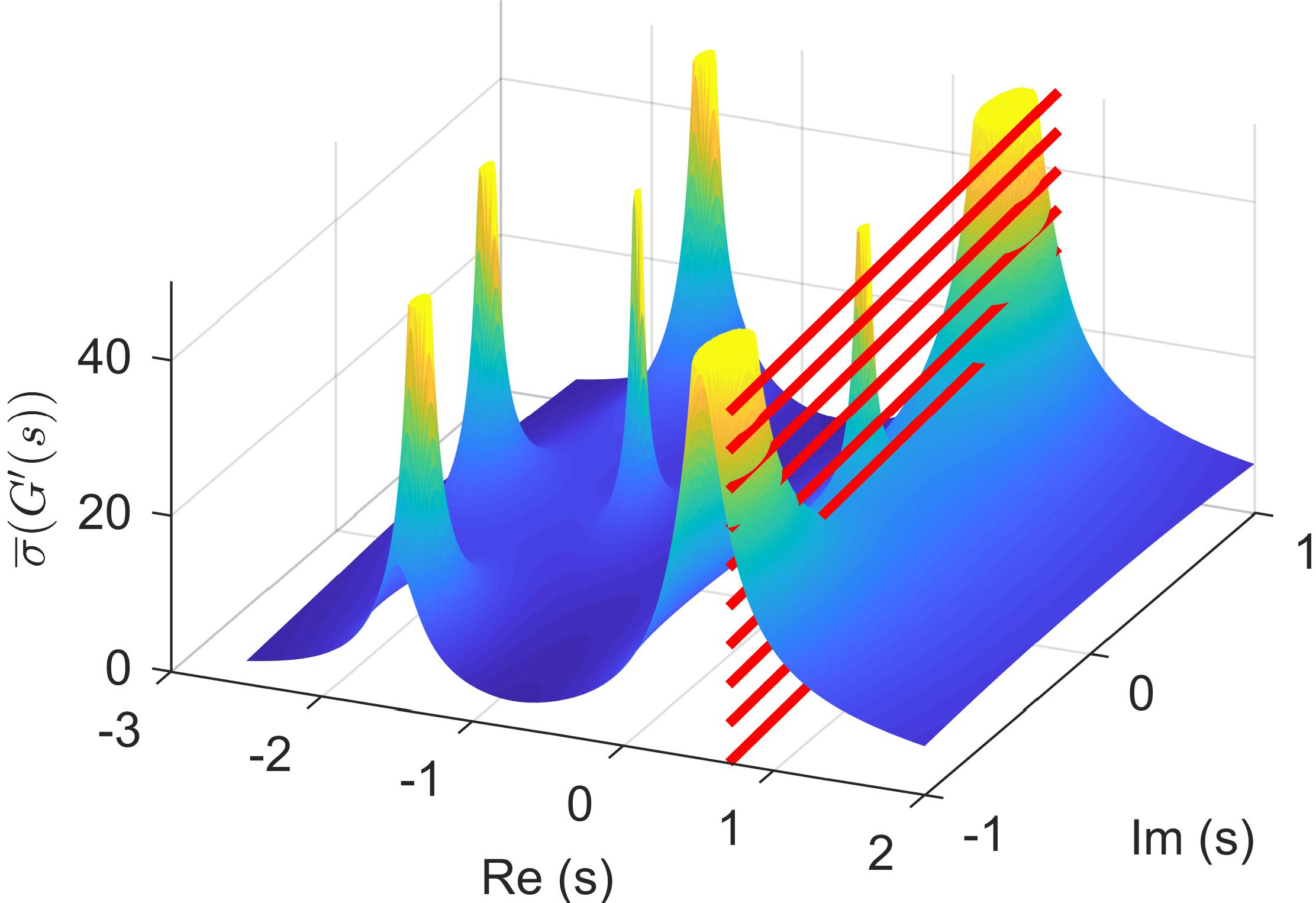
Red lines visualize the optimization curve , along which is evaluated. It shows that approaches high values in the proximity of system poles (Corollary 3.3).
Theorem 3.5
Given a detectable system with the set of poles that satisfies Assumption 1. Furthermore, assuming that no parameter-dependent pole-zero cancellations occur on . Then, will not cross during the minimization of .
Proof 3.6
The proof is analogous to the stability-certificate provided in (Mešanović et al. 2019) and is not shown in detail due to page limitations. It is based on the fact that, due to Assumption 1, is a continuous function of , and cannot discretely “jump over” . Thus, for to cross , would have to be increased to very high values (Corollary 3.3) in at least one step during the minimization, which is not allowed by the optimization method.
The assumption about pole-zero cancellations does not restrict generality, because if this occurs, can be shifted to avoid the cancellation and the minimization can be repeated.
Theorem 3.7 (pole shifting)
Given a detectable system
, with the set of poles , and an optimization curve . Furthermore, given two parameterizations and and any pole such that is sufficiently small and that and are reached in the neighborhood of .
Under Assumption 1,
if is sufficiently smaller than ,
the distance of to is greater than the distance of to , i.e.
| (14) |
Proof 3.8
Note that a sufficient value for depends on the parameter dependency of : ideally, if changes of remain small, (17) is equivalent to . From (15), it follows that in a neighborhood of . Thus, can be chosen sufficiently close to , such that the steepest descent direction during optimization leads to the displacement of , instead of the minimization of .
The following consequence arises from Theorem 3.7:
Corollary 3.9
The minimization of the norm of a stable system , i.e. , improves damping of poles which are sufficiently close to the imaginary axis.
Proof 3.10
The proof is obtained by inserting into Theorem 3.7. For this case, , and its minimization will push the poles away from the imaginary axis.
The previous theorem shows that minimization of will displace sufficiently close poles away from . However, an appropriate method to minimize is needed. We propose to do so by applying a similar optimization procedure as presented in (Mešanović et al. 2019).
Theorem 3.11 ( minimization)
Given a detectable multiple-input-multiple-output system with the transfer function which satisfies Assumption 1. Furthermore, given a continuous function , . Assuming there are no cancellations of parameter-dependent poles and zeros on , the solution of
| (18a) | ||||
| s.t. | (18b) | |||
| (18c) | ||||
minimizes for the sampling set . Here and are box constraints on the controller parameters, which may be .
Proof 3.12
Note that does not have to span the entire . It only needs to be defined around poles which are close to , where is reached. Furthermore, does not have to be infinitely dense. Due to Corollary 3.3, it suffices that , such that is in a sufficiently small neighborhood of . This way, the rise of due to is captured by the discretization. Thus, only several values need to be in around poles close to , which allows for efficient optimization.
However, Problem (18) is still non-convex due to the nonlinear parameter dependency in . To use linear matrix inequality solvers, we transform (18) into a series of convex optimization problems. In each iteration, is linearized around the parameter vector from the previous iteration, and is obtained. The following problem is then iteratively solved
| (22a) | ||||
| (22b) | ||||
| (22c) | ||||
Here the last constraint is added to preserve the linearization accuracy. Algorithm 1 summarizes the proposed approach to minimize .
For the proposed iterative pole placement approach, a suitable is chosen in each iteration, such that minimization of pushes the poles towards the target region.
In the following, we focus on the question of stabilization, for which the target region for all poles is the left half-plane, as this case is considered in subsequent numerical studies. To this end, a family of vertical lines, described with , is considered. To stabilize the system, is gradually reduced until all poles are in the left half-plane, as illustrated in Fig. 3.
Algorithm 2 outlines the proposed algorithm to achieve stability.
In the -th iteration, the pole with the maximal real value is calculated. Then, is chosen such that the maximum of is reached in the neighborhood of . Thereby, should be greater than to push the poles to the left half-plane. The algorithm terminates when all poles are in the left half-plane. Determining is important for the efficiency of the algorithm. If it is too small, must be minimized by a large amount to push the pole away, due to the high local gradients around poles. On the other hand, if it is too far from , will not be reached in the neighborhood of , and minimization of is not guaranteed to push the pole away from . We determine by first finding the largest value via a line-search, such that the maximum of is still achieved in the neighborhood of . Then, we set , which solves both of the previous issues in the considered numerical examples.
4 Application examples
We show the applicability of the approach on three systems with different initial parameterizations11 1 For the optimization, we use a Windows computer with an Intel® i7-4810MQ CPU running at 2.8 GHz and with 8 GB of RAM.. Note that the presented computation times should only give a reference about the computational complexity, as more tailored methods and special hardware would allow to further decrease the computation time. All controllers in the considered systems are purely local with different structures.
4.1 Four power plant model
We first consider a four power plant system, c.f. (Kundur 1993), as shown in Fig. 5. Detailed parameters of the system and the initial controller parameterization can be found in (Mešanović et al. 2017). The system consists of 56 states and 32 controller parameters. Static prosumers, representing disturbance inputs, are marked blue in Fig. 5.
For comparison, we use an approach which is based on the use of a Lyapunov matrix in the optimization problem, where the condition is used for stability. It is solved using an iterative coordinate-descent method, often called PK iteration, with iterative parameter linearization. Subsequently, we denote this as the PK method.
| Init. param. | # unst. poles | Comp. time | # iter. | |
|---|---|---|---|---|
| 2 | 0.058 | 1.8 s | 1 | |
| 2 | 0.43 | 5 s | 1 | |
| 5 | 1.3 | 6.4 s | 2 |
| Init. param. | # unst. poles | Comp. time | # iter. | |
|---|---|---|---|---|
| 2 | 0.058 | 180 s | 6 | |
| 2 | 0.43 | 215 s | 7 |
Table 1 shows the results of the optimization with the proposed singular value (SV) method for different unstable initial parameterizations, obtained by multiplying with a scaling factor. The computation time depends on , as more iterations are necessary if the unstable poles have a larger real part. For the three tested parameterizations, the SV method stabilized the system in 1.8 s, 5 s, and 6.4 s, respectively. On the other hand, the PK method, whose results are shown in Table 2, required 180 s, and 215 s, respectively, while it could not stabilize the system in the third case. Improvements per iteration for the SV and PK method are shown in Fig 6. Thus, the SV method significantly outperforms the PK method for this system.
4.2 The IEEE 39 bus 10 power plant model
We next consider the IEEE 39-bus system, consisting of 10 power plants, c.f. Fig 7. The parameters of the system can be found in (Mešanović et al. 2017). It consists of 190 states and 100 controller parameters. We denote the initial controller parameterization from (Mešanović et al. 2017) as .
| Init. param. | # unst. poles | Comp. time | # iter. | |
|---|---|---|---|---|
| 7 | 0.54 | 19 s | 5 | |
| 11 | 1.83 | 24 s | 4 | |
| 12 | 4.7 | 65 s | 12 | |
| 18 | 17.9 | 259 s | 12 |
Table 3 shows the computation results with the SV method. It shows that, even when the poles are far in the right half-plane, a stabilizing parameterization can be found in less than 5 minutes. Even though the approach requires the same amount of iterations to stabilize the system with and , the computation times are different because the internal minimization of requires more time per iteration for . For a system of this size, the PK method did not provide any results within reasonable time. Figure 8 shows the improvement in each iteration for the considered system.
4.3 European 53 power plant model
Finally, we consider a model with 53 power plants and 35 buses, developed within the research project DynaGridCenter 2020. The controllers used for this model are presented in (Mešanović et al. 2019). A more detailed description of the considered system cannot be presented due to space limitations. The system has a total of 469 states, 116 controller parameters, and 15 disturbance inputs.
| Init. param. | # unst. poles | Comp. time | # iter. | |
|---|---|---|---|---|
| 4 | 0.26 | 250 s | 1 | |
| 4 | 0.5 | 470 s | 2 |
Table 4 shows the computation results with the SV method for two initial parameterizations. Note that the computation times are significantly impacted by the calculation of in each iteration, requiring from 50 s to 100 s per iteration. Still, the SV method can find a stabilizing solution for this large system in a reasonable time frame.
5 Conclusion
As the share of renewable generation in power system rises, new methods for power system control become necessary to reduce the risk for a blackout. We proposed an approach for pole placement formulated in the frequency domain. As it does not introduce a Lyapunov matrix, the approach generally scales nicely. Nonlinear parameter dependencies can be considered as well. The approach is based on iterative minimization of the largest singular value along an optimization curve. The applicability of the approach was demonstrated in three simulation studies with different initial parameterizations. Future work will consider more efficient methods to determine , as well as validation for other target regions.
References
- Al Ali et al. (2014) Al Ali, S., Haase, T., Nassar, I., and Weber, H. (2014). Impact of increasing wind power generation on the north-south inter-area oscillation mode in the European ENTSO-E system. IFAC Proceedings Volumes, 47(3), 7653–7658.
- Apkarian and Noll (2018) Apkarian, P. and Noll, D. (2018). Structured -control of infinite-dimensional systems. International Journal of Robust and Nonlinear Control, 28(9), 3212–3238.
- Bamieh et al. (2002) Bamieh, B., Paganini, F., and Dahleh, M. (2002). Distributed control of spatially invariant systems. IEEE Trans. Auto. Cont., 47(7), 1091–1107.
- Befekadu and Erlich (2006) Befekadu, G. and Erlich, I. (2006). Robust decentralized controller design for power systems using matrix inequalities approaches. In Power Eng. Soc. General Meet. IEEE.
- Benner et al. (2018) Benner, P., Mitchell, T., and Overton, M. (2018). Low-order control design using a reduced-order model with a stability constraint on the full-order model. In 2018 IEEE Conf. on Decision and Control, 3000–3005.
- Chilali and Gahinet (1996) Chilali, M. and Gahinet, P. (1996). design with pole placement constraints: An LMI approach. IEEE Trans. Auto. Cont., 41(3), 358–367.
- Crivellaro et al. (2019) Crivellaro, A., Tayyebi, A., Gavriluta, C., Groß, D., Anta, A., Kupzog, F., and Dörfler, F. (2019). Beyond low-inertia systems: Massive integration of grid-forming power converters in transmission grids. arXiv preprint arXiv:1911.02870.
- De Moor and Boyd (1989) De Moor, B. and Boyd, S. (1989). Analytic properties of singular values and vectors. KTH Leuven, Belgium Tech. Rep, 28, 1989.
- DynaGridCenter (2020) DynaGridCenter (2020). Dynagridcenter. http://forschung-stromnetze.info/projekte/ dynamische-stromnetze-sicher-beherrschen/.
- Hopcroft and Kannan (2012) Hopcroft, J. and Kannan, R. (2012). Computer science theory for the information age. URL https://www.cs.cmu.edu/ venkatg/teaching/ CStheory-infoage/.
- IEEE (2006) IEEE (2006). IEEE recommended practice for excitation system models for power system stability studies. IEEE Std 421.5-2005 (Revision of IEEE Std 421.5-1992), 1–93. 10.1109/IEEESTD.2006.99499.
- Kammer and Karimi (2017) Kammer, C. and Karimi, A. (2017). Decentralized and distributed transient control for microgrids. IEEE Trans. Cont. Syst. Tech., (99), 1–12.
- Kundur (1993) Kundur, P. (1993). Power System Stability and Control. McGraw-Hill.
- Lunze (2013) Lunze, J. (2013). Regelungstechnik 2: Mehrgrößensysteme Digitale Regelung. Springer-Verlag.
- Marinescu et al. (2009) Marinescu, B., Mallem, B., Bourles, H., and Rouco, L. (2009). Robust coordinated tuning of parameters of standard power system stabilizers for local and global grid objectives. In PowerTech, Bucharest. IEEE.
- Mešanović et al. (2017) Mešanović, A., Münz, U., and Findeisen, R. (2017). Coordinated tuning of synchronous generator controllers for power oscillation damping. In Innovative Smart Grid Technologies Conference Europe. IEEE.
- Mešanović et al. (2019) Mešanović, A., Münz, U., Szabo, A., Mangold, M., Bamberger, J., Metzger, M., Heyde, C., Krebs, R., and Findeisen, R. (2019). Guaranteed controller parameter tuning for power systems: Method and experimental evaluation. submitted. URL https://arxiv.org/abs/1910.12335.
- Mešanović et al. (2018) Mešanović, A., Unseld, D., Münz, U., Ebenbauer, C., and Findeisen, R. (2018). Parameter tuning and optimal design of decentralized structured controllers for power oscillation damping in electrical networks. In Proc. Amer. Cont. Conf. (ACC), 3828–3833. IEEE.
- Nayyar et al. (2013) Nayyar, A., Mahajan, A., and Teneketzis, D. (2013). Decentralized stochastic control with partial history sharing: A common information approach. IEEE Trans. Auto. Cont., 58(7), 1644–1658.
- Poolla et al. (2019) Poolla, B., Gross, D., and Dörfler, F. (2019). Placement and implementation of grid-forming and grid-following virtual inertia and fast frequency response. IEEE Trans. Pow. Sys.
- Rotkowitz and Lall (2005) Rotkowitz, M. and Lall, S. (2005). A characterization of convex problems in decentralized control. IEEE Trans. Auto. Cont., 50(12), 1984–1996.
- Scherer and Weiland (2019) Scherer, C. and Weiland, S. (2019). Linear matrix inequalities in control, lecture notes. URL https://www.imng.uni-stuttgart.de/mst/files/ LectureNotes.pdf.
- Wang et al. (2019) Wang, Y., Matni, N., and Doyle, J. (2019). A system level approach to controller synthesis. IEEE Trans. Auto. Cont.
- Youla et al. (1976) Youla, D., Jabr, H., and Bongiorno, J. (1976). Modern Wiener-Hopf design of optimal controllers–part II: The multivariable case. IEEE Trans. Auto. Cont., 21(3), 319–338.
- Zheng et al. (2019) Zheng, Y., Furieri, L., Kamgarpour, M., and Li, N. (2019). On the parameterization of stabilizing controllers using closed-loop responses. arXiv preprint arXiv:1909.12346.