Inferring Vector Magnetic Fields from Stokes Profiles of GST/NIRIS Using a Convolutional Neural NetworkFacilities: Big Bear Solar Observatory

We conducted a series of experiments to evaluate the performance of the proposed CNN model and compare it with related methods based on four performance metrics: mean absolute error (Sen & Srivastava 1990, MAE;), percent agreement (McHugh 2012, PA;), R-squared (Sen & Srivastava 1990) and Pearson product-moment correlation coefficient (Galton 1886; Pearson 1895, PPMCC;). We considered six quantities: total magnetic field strength ($B_{total}$), inclination angle ($\phi$), azimuth angle ($\theta$), $B_{x}$, $B_{y}$ and $B_{z}$. For each quantity, we compared its ME-calculated values with our CNN-inferred values and computed the four performance metrics.

The first performance metric is defined as (Sen & Srivastava 1990):

where $N$ is the total number of data samples (pixels) in a test image, and $y_{i}$ ($\hat{y}_{i}$, respectively) denotes the ME-calculated (CNN-inferred, respectively) value for the $i$th pixel in the test image. This metric is used to quantitatively assess the dissimilarity (distance) between the ME-calculated values and CNN-inferred values in the test image. The smaller the MAE is, the better performance a method has.

The second performance metric is defined as (McHugh 2012):

where $M$ denotes the total number of agreement pixels in the test image. We say the $i$th pixel in the test image is an agreement pixel if $|y_{i}-\hat{y}_{i}|$ is smaller than a user-specified threshold. (The default thresholds are set to 200 Gauss for $B_{total}$, $B_{x}$, $B_{y}$, $B_{z}$ respectively and 10 degree for $\phi$, $\theta$ respectively.) This metric is used to quantitatively assess the similarity between the ME-calculated values and CNN-inferred values in the test image. The larger the PA is, the better performance a method has.

The third performance metric is defined as (Sen & Srivastava 1990):

where $\overline{y}=\frac{1}{N}\sum_{i=1}^{N}y_{i}$ denotes the mean of the ME-calculated values for all the pixels in the test image. The R-squared value, ranging from $-\infty$ to 1, is used to measure the strength of the relationship between the ME-calculated values and CNN-inferred values in the test image. The larger (i.e., the closer to 1) the R-squared value is, the stronger relationship between the ME-calculated values and CNN-inferred values we have.

The fourth performance metric is defined as (Galton 1886; Pearson 1895):

where $X$ and $Y$ represent the ME-calculated values and CNN-inferred values respectively, $\mu_{X}$ and $\mu_{Y}$ are the mean of $X$ and $Y$ respectively, $\sigma_{X}$ and $\sigma_{Y}$ are the standard deviation of $X$ and $Y$ respectively, and $E(\cdot)$ is the expectation. The value of PPMCC ranges from $-1$ to 1. A value of 1 means that a linear equation describes the relationship between $X$ and $Y$ perfectly where all data points lying on a line for which $Y$ increases as $X$ increases. A value of $-1$ means that all data points lie on a line for which $Y$ decreases as $X$ increases. A value of 0 means that there is no linear correlation between the variables $X$ and $Y$. We will mainly use PPMCC in our experimental study because it measures the linear correlation between the ME-calculated values and CNN-inferred values, quantifying how well the CNN-inferred values agree with the ME-calculated values in the test image (Galton 1886; Pearson 1895; Sen & Srivastava 1990). The larger (i.e., the closer to 1) the PPMCC is, the better performance a method has. Notice that PA, R-squared and PPMCC do not have units while MAE has units: “Gauss” for $B_{total}$, $B_{x}$, $B_{y}$, $B_{z}$ respectively and “degree” for $\phi$ (inclination angle), $\theta$ (azimuth angle) respectively.

In this experiment, we used the one million data samples (pixels) from AR 12371 collected on 2015 June 22 as the training data to train our CNN model. We then used the trained CNN model to infer vector magnetic fields from the Stokes Q, U, V profiles of the pixels in the three test sets (images) described in Section II.¹¹ 1 The source code and datasets used in the experiment can be downloaded from https://web.njit.edu/~wangj/CNNStokesInversion/. For comparison purposes, we also used the Milne-Eddington (ME) method (Auer et al. 1977; Landi Degl’Innocenti 1984) to derive the vector magnetic fields of the pixels in the three test images.

Figure 3 (Figure 4, Figure 5 respectively) presents results for the three obtained quantities $B_{total}$, $\phi$ (inclination angle) and $\theta$ (azimuth angle), displayed from top to bottom in the figure, of the test image with 720$\times$720 pixels from AR 12371 (AR 12665, AR 12673 respectively) collected on 2015 June 25 20:00:00 UT (2017 July 13 18:35:00 UT, 2017 September 6 19:18:00 UT respectively). In all the figures, the first column shows scatter plots for each obtained quantity. The X-axis and Y-axis in each scatter plot represent the values obtained by the ME method and CNN method respectively. The black diagonal line in each scatter plot corresponds to pixels whose ME-calculated values are identical to CNN-inferred values. The second columns in these figures show magnetic maps with 720$\times$720 pixels derived by the ME method. The third columns in the figures show magnetic maps with 720$\times$720 pixels inferred by our CNN method.

Summary of the results. The scatter plots in the figures show that the Stokes inversion results obtained by our CNN method and the ME method are highly correlated. From the top-left panels in Figures 3, 4 and 5, we see that the CNN-inferred $B_{total}$ values are closer to the ME-calculated $B_{total}$ values in the low-field end and are farther from the ME-calculated $B_{total}$ values in the high-field end. The figures also show that the CNN method produces smoother and cleaner magnetic maps than the ME method. There are salt-pepper noise pixels in the magnetic maps produced by the ME method. To help locate the noise pixels, we use percentage difference images in which the value of the $i$th pixel is equal to $(y_{i}-\hat{y}_{i})$/$y_{i}$ $\times$ 100% where $y_{i}$ ($\hat{y}_{i}$, respectively) denotes the ME-calculated (CNN-inferred, respectively) value for the $i$th pixel. For example, Figure 6 shows the percentage difference images for the $\phi$ (inclination angle) maps in Figures 3, 4 and 5. The percentage difference images highlight the locations of the differences between the CNN-inferred $\phi$ values and ME-calculated $\phi$ values in the test images. Figure 7 (Figure 8, Figure 9 respectively) in the Appendix presents results for the quantities $B_{x}$, $B_{y}$ and $B_{z}$, displayed from top to bottom in the figure, of the test image with 720$\times$720 pixels from AR 12371 (AR 12665, AR 12673 respectively) collected on 2015 June 25 20:00:00 UT (2017 July 13 18:35:00 UT, 2017 September 6 19:18:00 UT respectively).

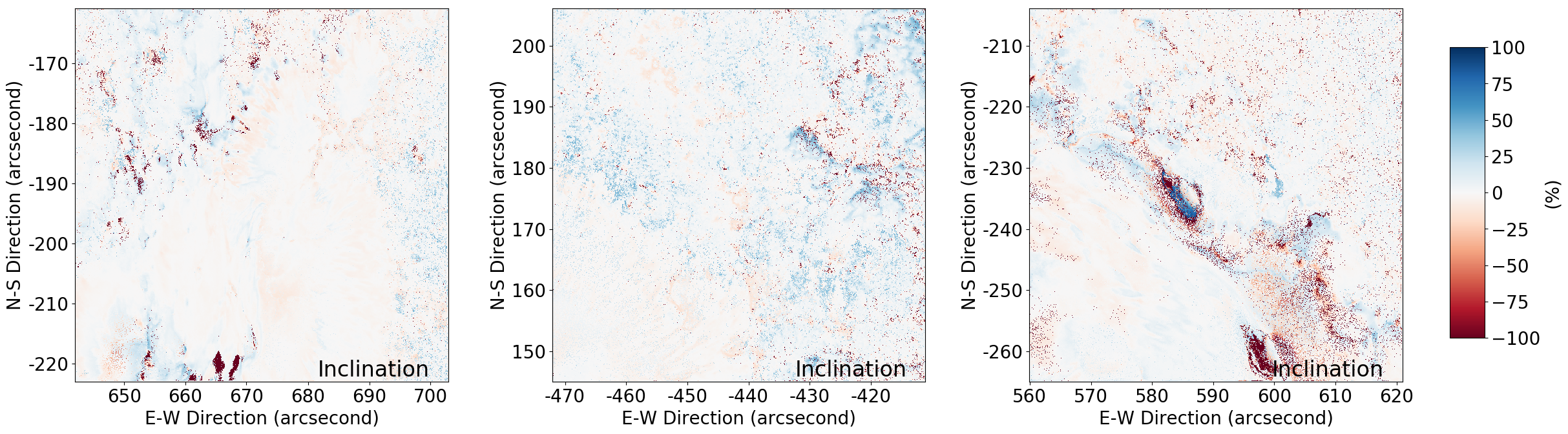
To quantitatively assess the number of noise pixels in the magnetic maps derived by the ME and CNN methods, we adopt a threshold-based algorithm, which works as follows. We define $P$ to be a noise pixel (outlier) with respect to a user-specified threshold if among $P$’s eight neighboring pixels, there are more than four neighboring pixels satisfying the following condition: the difference between the value of a neighboring pixel and the value of $P$ is greater than or equal to the threshold. The default thresholds are set to 500 Gauss for $B_{total}$, $B_{x}$, $B_{y}$, $B_{z}$ respectively and 20 degree for $\phi$ (inclination angle), $\theta$ (azimuth angle) respectively. We define the outlier-difference to be the number of outliers produced by the ME method minus the number of outliers produced by our CNN method. A positive outlier-difference means ME produces more outliers than CNN while a negative outlier-difference means CNN produces more outliers than ME.

Table 1 presents the performance metric values of the CNN method. The results in Table 1 are consistent with those in Figures 3-9. Specifically, the CNN-inferred results are highly correlated to the ME-calculated results with PPMCC values being close to 1. Furthermore, CNN produces smoother magnetic maps with fewer outliers (noise pixels) than the ME method. This happens because among the one million training data samples whose labels are calculated by the ME method, there are relatively few outliers. The CNN method can learn latent patterns from the majority of the training data samples, which are clean. As a consequence, we obtain a good CNN model capable of producing clean results. Tables 5 and 6 in the Appendix present the performance metric values for the test images from AR 12371 and AR 12665 collected at ten different time points on 2015 June 25 and 2017 July 13 respectively. The results in these tables are consistent with those in Table 1.

Comparison with related methods. To further understand the behavior of our CNN method and compare it with related machine learning algorithms, we conduct a cross-validation study as follows. We partition the training set of one million data samples from AR 12371 on 2015 June 22 into 10 equal-sized folds. For every two training folds $i$ and $j$, $i$ $\neq$ $j$, fold $i$ and fold $j$ are disjoint. The first test set contains the ten 720$\times$720 images, also from AR 12371, collected on 2015 June 25. These test images are numbered from 1 to 10. In run $i$, 1 $\leq$ $i$ $\leq$ 10, all training data samples except those in training fold $i$ are used to train a machine learning model, and the trained model is then used to make predictions on test image $i$. We calculate the performance metrics MAE, PA, R-squared, PPMCC and outlier-difference based on the predictions made in run $i$. There are 10 runs. The means and standard deviations over the 10 runs are calculated and recorded. We also conduct the same cross-validation study for the second test set containing the ten 720$\times$720 images from AR 12665 collected on 2017 July 13, and the third test set containing the 720$\times$720 image from AR 12673 collected on 2017 September 6. The third test set has only one image, and hence in each run, the same test image is used.

The related machine learning algorithms considered here include multiple support vector regression (Rees et al. 2004; Teng 2015, MSVR;) and multilayer perceptrons (Carroll & Staude 2001; Socas-Navarro 2003; Socas-Navarro 2005; Carroll & Kopf 2008, MLP;). The MSVR method uses the radial basis function (RBF) kernel. The MLP model consists of an input layer, an output layer and two hidden layers both with 1024 neurons. Table 2 (Table 3, Table 4 respectively) presents the mean MAE, PA, R-squared, PPMCC, outlier-difference and standard deviation for each quantity $B_{total}$, $B_{x}$, $B_{y}$, $B_{z}$, $\phi$ (inclination angle), $\theta$ (azimuth angle) inferred by each of the three machine learning methods MSVR, MLP and our CNN for the first (second, third respectively) test set. In the tables, PA, R-squared, PPMCC and outlier-difference do not have units while MAE has units: “Gauss” for $B_{total}$, $B_{x}$, $B_{y}$, $B_{z}$ respectively and “degree” for $\phi$ (inclination angle), $\theta$ (azimuth angle) respectively. It can be seen from the tables that the CNN-inferred results are highly correlated to the ME-calculated results and are closer to the ME’s results with PPMCC values being closer to 1 on average than those from the other two machine learning methods. In particular, based on the calculations on the six quantities $B_{total}$, $B_{x}$, $B_{y}$, $B_{z}$, $\phi$ (inclination angle) and $\theta$ (azimuth angle) in Tables 2-4, our CNN method outperforms the current best machine learning method (MLP) by 2.6% on average in PPMCC. However, there is no definite conclusion about outlier-differences among the three machine learning methods.

In the previous subsection we use data points (pixels) from AR 12371 on 2015 June 22 as training data. In this subsection we conduct additional experiments by varying training data as follows. There are four datasets $\text{D}_{1}$, $\text{D}_{2}$, $\text{D}_{3}$, $\text{D}_{4}$ containing the images from AR 12371 on 2015 June 22, AR 12371 on 2015 June 25, AR 12665 on 2017 July 13, and AR 12673 on 2017 September 6 respectively. In each experiment we randomly select one million pixels (data samples) from one or more datasets to form a training set. The CNN model is trained on this training set and the trained model is then used to perform Stokes inversion on a test image. This test image must be from a dataset that is different from those datasets used to construct the training set. The time point for the test image is 17:33:00 UT on 2015 June 22, 20:00:00 UT on 2015 June 25, 18:35:00 UT on 2017 July 13, and 19:18:00 UT on 2017 September 6 respectively. We use $\text{D}^{\text{train}}_{x}\rightarrow\text{D}^{\text{test}}_{w}$ ($\text{D}^{\text{train}}_{x,y}\rightarrow\text{D}^{\text{test}}_{w}$, $\text{D}^{\text{train}}_{x,y,z}\rightarrow\text{D}^{\text{test}}_{w}$ respectively) to represent the experiment that uses training data samples from $\text{D}_{x}$ (training data samples from $\text{D}_{x}$ and $\text{D}_{y}$, training data samples from $\text{D}_{x}$, $\text{D}_{y}$ and $\text{D}_{z}$ respectively) and test data samples (pixels) from $\text{D}_{w}$ where $1\leq x,y,z,w\leq 4$. Because $\text{D}_{4}$ has only one 720$\times$720 image with 518400 pixels, $\text{D}_{4}$ alone is not used as a training set. Hence, there are 25 experiments in total. In each experiment, we calculate the performance metrics MAE, PA, R-squared, PPMCC and outlier-difference. Tables 7$-$10 in the Appendix present the experimental results. Major findings based on these tables are summarized below.

1. Our CNN-inferred results and ME-calculated results are highly correlated and close to each other with a PPMCC of $\sim$0.9 or higher for the total magnetic field strength, regardless of whether the training and test data used by the CNN method are from the same active region (AR) or different ARs, or whether the training and test data are close (e.g., within $\sim$3 days) or distant (e.g., over 2 years) in time. This finding can be seen from Tables 7-10 where the PPMCC of $B_{total}$ in $\text{D}^{\text{train}}_{2}\rightarrow\text{D}^{\text{test}}_{1}$ ($\text{D}^{\text{train}}_{3}\rightarrow\text{D}^{\text{test}}_{1}$, $\text{D}^{\text{train}}_{1}\rightarrow\text{D}^{\text{test}}_{2}$, $\text{D}^{\text{train}}_{3}\rightarrow\text{D}^{\text{test}}_{2}$, $\text{D}^{\text{train}}_{1}\rightarrow\text{D}^{\text{test}}_{3}$, $\text{D}^{\text{train}}_{2}\rightarrow\text{D}^{\text{test}}_{3}$, $\text{D}^{\text{train}}_{1}\rightarrow\text{D}^{\text{test}}_{4}$, $\text{D}^{\text{train}}_{2}\rightarrow\text{D}^{\text{test}}_{4}$, and $\text{D}^{\text{train}}_{3}\rightarrow\text{D}^{\text{test}}_{4}$, respectively) is 0.956 (0.924, 0.983, 0.951, 0.976, 0.979, 0.936, 0.927, and 0.896, respectively).

2. With respect to the same test image, using the training data from the same AR in which the test image is taken yields a better result with a higher PPMCC than using the training and test data that are from different ARs. This finding can be seen from Tables 7 and 8 where the PPMCC of $B_{total}$ in $\text{D}^{\text{train}}_{2}\rightarrow\text{D}^{\text{test}}_{1}$ is 0.956, which is greater than the PPMCC of $B_{total}$, 0.924, in $\text{D}^{\text{train}}_{3}\rightarrow\text{D}^{\text{test}}_{1}$. Moreover, the PPMCC of $B_{total}$ in $\text{D}^{\text{train}}_{1}\rightarrow\text{D}^{\text{test}}_{2}$ is 0.983, which is greater than the PPMCC of $B_{total}$, 0.951, in $\text{D}^{\text{train}}_{3}\rightarrow\text{D}^{\text{test}}_{2}$.

3. However, with respect to the same test image, using the training and test data that are close in time does not necessarily yield a better result than using the training and test data that are distant in time. This finding can be seen from Table 10 where the PPMCC of $B_{total}$ in $\text{D}^{\text{train}}_{1}\rightarrow\text{D}^{\text{test}}_{4}$ is 0.936, which is greater than the PPMCC of $B_{total}$, 0.896, in $\text{D}^{\text{train}}_{3}\rightarrow\text{D}^{\text{test}}_{4}$, though $D_{3}$ is closer to $D_{4}$ than $D_{1}$ in time.

4. From Tables 7-10, we can see that the CNN-inferred results have much fewer outliers than the ME-calculated results for all of $B_{total}$, $B_{x}$, $B_{y}$, $B_{z}$, $\phi$, $\theta$ in all the experiments except for $B_{y}$ in Table 8. This finding is consistent with the results reported in Table 1.

References

- Asensio Ramos & de la Cruz Rodríguez (2015) Asensio Ramos, A., & de la Cruz Rodríguez, J. 2015, A&A, 577, A140, doi: 10.1051/0004-6361/201425508
- Asensio Ramos & Díaz Baso (2019) Asensio Ramos, A., & Díaz Baso, C. J. 2019, A&A, 626, A102, doi: 10.1051/0004-6361/201935628
- Auer et al. (1977) Auer, L. H., Heasley, J. N., & House, L. L. 1977, Sol. Phys., 55, 47, doi: 10.1007/bf00150873
- Borrero et al. (2011) Borrero, J. M., Tomczyk, S., Kubo, M., et al. 2011, Sol. Phys., 273, 267, doi: 10.1007/s11207-010-9515-6
- Cao et al. (2012) Cao, W., Goode, P. R., Ahn, K., et al. 2012, Astronomical Society of the Pacific Conference Series, Vol. 463, NIRIS: The Second Generation Near-Infrared Imaging Spectro-polarimeter for the 1.6 Meter New Solar Telescope, ed. T. R. Rimmele, A. Tritschler, F. Wöger, M. Collados Vera, H. Socas-Navarro, R. Schlichenmaier, M. Carlsson, T. Berger, A. Cadavid, P. R. Gilbert, P. R. Goode, & M. Knölker, 291
- Cao et al. (2006) Cao, W., Jing, J., Ma, J., et al. 2006, PASP, 118, 838, doi: 10.1086/505408
- Carroll & Kopf (2008) Carroll, T. A., & Kopf, M. 2008, A&A, 481, L37, doi: 10.1051/0004-6361:20079197
- Carroll & Staude (2001) Carroll, T. A., & Staude, J. 2001, A&A, 378, 316, doi: 10.1051/0004-6361:20011167
- Collados (2008) Collados, M. 2008, in Ground-based and Airborne Telescopes II, ed. L. M. Stepp & R. Gilmozzi (SPIE). https://doi.org/10.1117%2F12.790105
- del Toro Iniesta & Ruiz Cobo (1996) del Toro Iniesta, J. C., & Ruiz Cobo, B. 1996, Sol. Phys., 164, 169, doi: 10.1007/bf00146631
- Frutiger et al. (2000) Frutiger, C., Solanki, S. K., Fligge, M., & Bruls, J. H. M. J. 2000, A&A, 358, 1109
- Galton (1886) Galton, F. 1886, The Journal of the Anthropological Institute of Great Britain and Ireland, 15, 246, doi: 10.2307/2841583
- Goode & Cao (2012) Goode, P. R., & Cao, W. 2012, Astronomical Society of the Pacific Conference Series, Vol. 463, The 1.6 m Off-Axis New Solar Telescope (NST) in Big Bear, ed. T. R. Rimmele, A. Tritschler, F. Wöger, M. Collados Vera, H. Socas-Navarro, R. Schlichenmaier, M. Carlsson, T. Berger, A. Cadavid, P. R. Gilbert, P. R. Goode, & M. Knölker, 357
- Goodfellow et al. (2016) Goodfellow, I. J., Bengio, Y., & Courville, A. C. 2016, Deep Learning, Adaptive computation and machine learning (MIT Press). http://www.deeplearningbook.org/
- Lagg et al. (2004) Lagg, A., Woch, J., Krupp, N., & Solanki, S. K. 2004, A&A, 414, 1109, doi: 10.1051/0004-6361:20031643
- Landi Degl’Innocenti (1984) Landi Degl’Innocenti, E. 1984, Sol. Phys., 91, 1, doi: 10.1007/bf00213606
- Landolfi et al. (1984) Landolfi, M., Landi Degl’innocenti, E., & Arena, P. 1984, Sol. Phys., 93, 269, doi: 10.1007/bf02270839
- LeCun et al. (2015) LeCun, Y., Bengio, Y., & Hinton, G. 2015, Nature, 521, 436, doi: 10.1038/nature14539
- Liu et al. (2018) Liu, C., Cao, W., Chae, J., et al. 2018, ApJ, 869, 21, doi: 10.3847/1538-4357/aaecd0
- McHugh (2012) McHugh, M. L. 2012, Biochemia Medica, 22, 276, doi: 10.11613/bm.2012.031
- McMullin et al. (2012) McMullin, J. P., Rimmele, T. R., Keil, S. L., et al. 2012, in Ground-based and Airborne Telescopes IV, ed. L. M. Stepp, R. Gilmozzi, & H. J. Hall (SPIE). https://doi.org/10.1117%2F12.926949
- Pearson (1895) Pearson, K. 1895, Proceedings of the Royal Society of London, 58, 240, doi: 10.1098/rspl.1895.0041
- Press et al. (1991) Press, W. H., Flannery, B. P., Teukolsky, S. A., & Vetterling, W. T. 1991, Mathematics of Computation, 56, 396, doi: 10.2307/2008560
- Quintero Noda et al. (2015) Quintero Noda, C., Asensio Ramos, A., Orozco Suárez, D., & Ruiz Cobo, B. 2015, A&A, 579, A3, doi: 10.1051/0004-6361/201425414
- Rees et al. (2004) Rees, D., Guo, Y., López Ariste, A., & Graham, J. 2004, in Lecture Notes in Computer Science (Springer Berlin Heidelberg), 388–394. https://doi.org/10.1007%2F978-3-540-30134-9_52
- Ruiz Cobo & Asensio Ramos (2012) Ruiz Cobo, B., & Asensio Ramos, A. 2012, A&A, 549, L4, doi: 10.1051/0004-6361/201220373
- Ruiz Cobo & del Toro Iniesta (1992) Ruiz Cobo, B., & del Toro Iniesta, J. C. 1992, ApJ, 398, 375, doi: 10.1086/171862
- Sen & Srivastava (1990) Sen, A., & Srivastava, M. 1990, Regression Analysis (Springer-Verlag New York), doi: 10.1007/978-1-4612-4470-7
- Skumanich & Lites (1987) Skumanich, A., & Lites, B. W. 1987, ApJ, 322, 473, doi: 10.1086/165743
- Socas-Navarro (2003) Socas-Navarro, H. 2003, Neural Networks, 16, 355, doi: 10.1016/s0893-6080(03)00024-8
- Socas-Navarro (2005) —. 2005, ApJ, 621, 545, doi: 10.1086/427431
- Socas-Navarro et al. (2001) Socas-Navarro, H., López Ariste, A., & Lites, B. W. 2001, ApJ, 553, 949, doi: 10.1086/320984
- Teng (2015) Teng, F. 2015, Sol. Phys., 290, 2693, doi: 10.1007/s11207-015-0781-1
- Unno (1956) Unno, W. 1956, Astronomical Society of Japan, 8, 108
- Wang et al. (2015) Wang, H., Cao, W., Liu, C., et al. 2015, Nature Communications, 6, doi: 10.1038/ncomms8008
- Wang et al. (2017) Wang, H., Liu, C., Ahn, K., et al. 2017, Nature Astronomy, 1, doi: 10.1038/s41550-017-0085
- Xu et al. (2016) Xu, Y., Cao, W., Ding, M., et al. 2016, ApJ, 819, 89, doi: 10.3847/0004-637x/819/2/89
- Xu et al. (2018) Xu, Y., Cao, W., Ahn, K., et al. 2018, Nature Communications, 9, doi: 10.1038/s41467-017-02509-w