The localization of non-backtracking centrality in networks
and its physical consequences

The NBC can be practically calculated by using the Ihara-Bass determinant formula bass1992; Martin2014, which shows that the NBC values $x_{i}$ correspond to the first $N$ elements of the PEV of the $2N\times 2N$ matrix

$$\mathbf{M}=\left(\begin{array}[]{cc}\mathbf{A}&\mathbf{I}-\mathbf{D}\\ \mathbf{I}&\mathbf{0}\end{array}\right),$$

(4)

where $\mathbf{A}$ is the adjacency matrix, $\mathbf{I}$ is the identity matrix, and $\mathbf{D}$ is a diagonal matrix of elements $D_{ij}=\delta_{ij}k_{i}$. Using the Ihara-Bass formalism PhysRevE.91.010801 (see Method M1) one can express, in full generality, the leading eigenvalue $\mu_{M}$ in terms of the NBC as

$$\mu_{M}=\frac{\sum_{i}k_{i}x_{i}}{\sum_{i}x_{i}}-1.$$

(5)

Following Ref. Martin2014 (see Method M1), it is possible to argue that, for uncorrelated random networks, i.e., networks with a given degree sequence but completely random in all other respects Newman10, the dependence of the components of the NB matrix PEV is

$$v_{j\to i}\sim k_{j}-1.$$

(6)

Introducing this relation into the definition of the NBC, Eq. (3), and applying the normalization $\sum_{i}x_{i}=1$, we obtain

$$x_{i}^{\mathrm{un}}=\frac{\sum_{j}A_{ij}(k_{j}-1)}{\sum_{j}k_{j}(k_{j}-1)},$$

(7)

that, inserted into Eq. (5), leads to

$$\mu_{M}^{\mathrm{un}}=\frac{\sum_{ij}(k_{i}-1)A_{ij}(k_{j}-1)}{\sum_{j}k_{j}(k_{j}-1)}.$$

(8)

These expressions constitute an improvement over previous results Krzakala2013; Martin2014; PhysRevE.91.010801, namely

$$x_{i}^{\mathrm{an}}=\frac{k_{i}}{\left\langle{k}\right\rangle N},\quad\mathrm{and}\quad\mu_{M}^{\mathrm{an}}=\frac{\left\langle{k^{2}}\right\rangle}{\left\langle{k}\right\rangle}-1,$$

(9)

($\left\langle{k^{n}}\right\rangle$ is the $n$-th moment of the degree distribution), which can be recovered from Eqs. (7) and (8) by replacing the network adjacency matrix with its annealed approximated value $\bar{A}_{ij}=k_{i}k_{j}/(\left\langle{k}\right\rangle N)$ Dorogovtsev2008; Boguna09.

We now check the predictions developed above with the LEV $\mu_{M}$ and the NBC $x_{i}$ determined numerically by applying the power iteration method golub2012matrix to the Ihara-Bass matrix $\mathbf{M}$ for random uncorrelated networks with a power-law degree distribution $P(k)\sim k^{-\gamma}$, generated using the uncorrelated configuration model (UCM) Catanzaro2005.

In Fig 1 we present, as a function of the network size $N$, a comparison between the NB LEV, $\mu_{M}$, evaluated numerically and our theoretical prediction Eq. (8). The match between theory and simulation is excellent. However, also Eq. (9) gives very accurate results, differing in average by less than $0.5\%$ from the theoretical result Eq. (8). A much more noticeable improvement is observed instead for the NB centrality $x_{i}$, for which annealed network approximation does not provide accurate predictions (see Fig. 2, bottom row). In Fig. 2 (top row) we show the dependence of the NBC $x_{i}$ on the structure of the adjacency matrix, as given by Eq. (7), namely $x_{i}\sim\sum_{j}A_{ij}(k_{j}-1)$. The analytical expression is extremely accurate for values of $\gamma<3$. For $\gamma>3$, although some scattering can be observed with respect to the expected value, the prediction is still good, much more accurate than the annealed network approximation. More evidence about the superior accuracy of our approach is found considering the inverse participation ratio $Y_{4}(N)$ as a function of network size (see Method M2).

The non-backtracking centrality was introduced with the goal of overcoming the flaws of eigenvector centrality, due to the localization of the adjacency matrix principal eigenvector on star graphs surrounding hubs of large degree, that artificially inflate their own eigenvector centrality Martin2014. For the NBC the addition of a large hub to an otherwise homogeneous network has a limited impact. Indeed, the addition of a dangling hub of degree $K$, connected to $K-1$ leaves of degree $1$ and to a generic network by a single edge, does not alter at all the value of $\mu_{M}$ Krzakala2013; Martin2014 (see Method M3). In the case of a hub integrated into the network, connected to $K$ other random nodes in the graph, Ref. Martin2014 argued, from the perspective of the annealed network approximation, that its effect is irrelevant in the thermodynamic limit. A more elaborate analysis (see Method M3) shows that this is true unless $K\gg(N/\left\langle{k}\right\rangle)^{1/2}$. Only in this case an integrated hub has an effect and leads to a PEV significantly larger than the PEV of the original network and scaling as $[\left\langle{k}\right\rangle K(K-1)/N]^{1/3}$.

However, it is possible that other types of subgraphs play for the NB centrality the same role that star graphs play for eigenvector centrality: They can have, alone, large values of $\mu_{M}$, so that, if present within an otherwise random network, they determine $\mu_{M}$ of the whole structure, with the overall NBC localized on them. We now show that these subgraphs actually exist and can have dramatic effects.

As noticed in Ref. Martin2014, the simplest example is a clique of size $K_{c}$, which is associated to $\mu_{M}^{\mathrm{clique}}=K_{c}-2$. If $K_{c}$ is large enough, $\mu_{M}^{\mathrm{clique}}$ can dominate over $\mu_{M}^{\mathrm{un}}$. But also a homogeneous (Poisson) subgraph of average degree $\left\langle{k}\right\rangle$, for which $\mu_{M}=\left\langle{k}\right\rangle$ Martin2014; Krzakala2013, can become the substrate of a localized NB PEV if $\left\langle{k}\right\rangle$ is sufficiently large.

Apart from these simple examples, a less trivial one is the case of overlapping hubs, i.e., a set of $n$ hubs of degree $K$, connected to the same $K$ leaves of degree $n$, see Supplementary Figure SF1. The intrinsic LEV associated to such a structure is (see Method M3)

$$\mu_{M}^{\mathrm{oh}}=\sqrt{(n-1)(K-1)}.$$

(10)

This last case is particularly important, since $\mu_{M}^{\mathrm{oh}}$ can become very large due to a few overlapping hubs of very large degree $K$, or due to a large number of hubs with moderate overlap $K$.

In Fig. 3(a) and 3(b) we compare the theoretical predictions derived for uncorrelated and annealed networks with the values of $\mu_{M}$ computed numerically for a set of 109 real-world networks of diverse origin (see Supplementary Table ST1 for details). In opposite ways, both predictions, $\mu_{M}^{\mathrm{an}}$ and $\mu_{M}^{\mathrm{un}}$, fail to provide an accurate approximation of empirical results for many networks. In the most noticeable cases, the networks Zhishi and DBpedia, the uncorrelated prediction Eq. (8) largely underestimates the value of $\mu_{M}$, while the annealed network prediction Eq. (9) largely overestimates it.

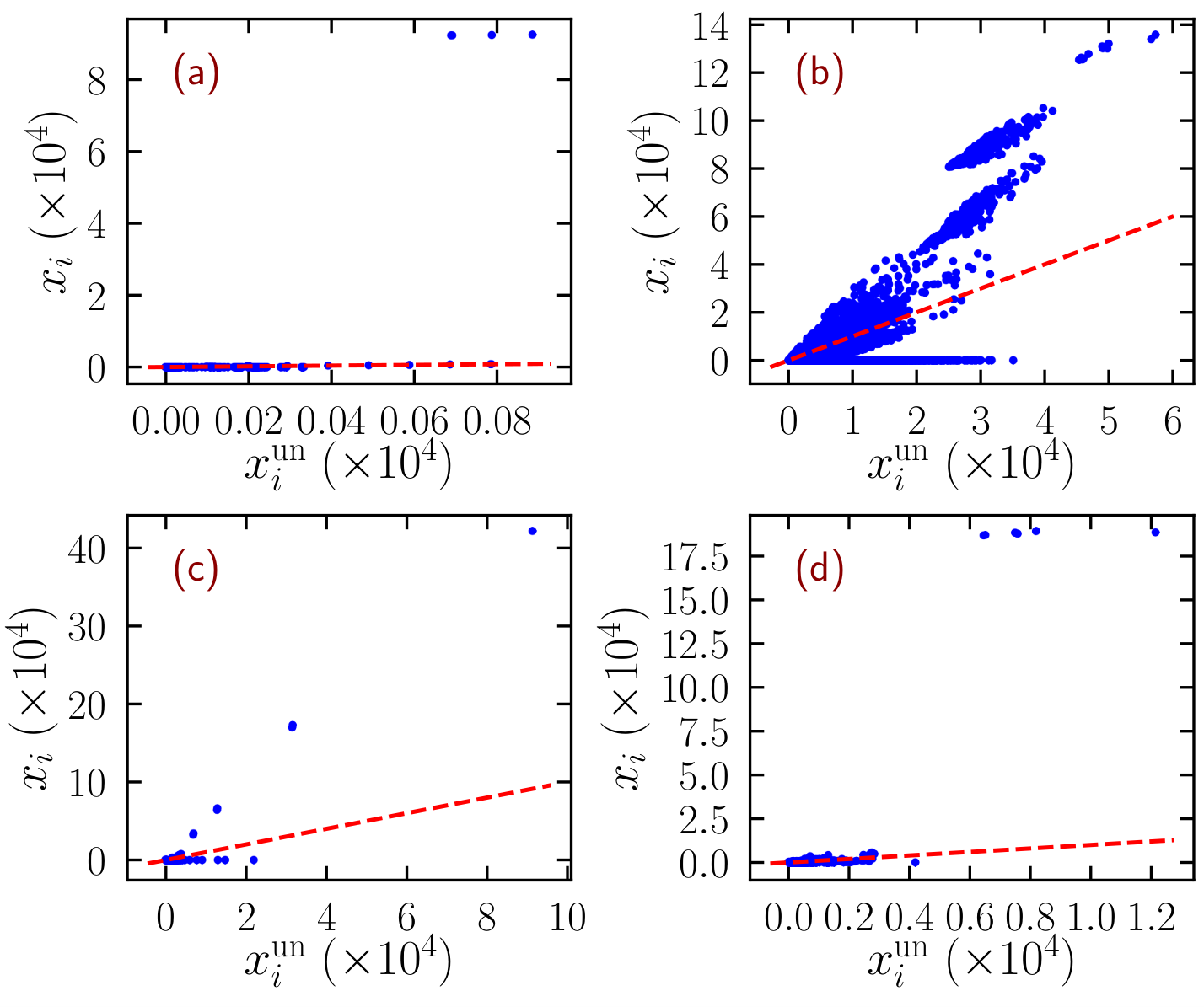
To shed light on the origin of these discrepancies, in Supplementary Figure SF2 we compare the empirical NBC, $x_{i}$, with the theoretical prediction $x_{i}^{\mathrm{un}}$ for four real-world networks in which the predictions largely fail. We observe that, in all networks, a few nodes assume an exceedingly large value of $x_{i}$, i.e., the NBC is localized on a very small subset of nodes, which includes the largest hubs.

It is clear that, in order to obtain an accurate prediction of $\mu_{M}$ in real-world networks, it is necessary to take into account the possible localization of the NB centrality on subgraphs which, despite being relatively small, may determine $\mu_{M}$ for the whole structure. In previous paragraphs, we have seen that two special subgraphs, a large clique/relatively dense homogeneous graph, or a set of overlapping hubs, may become the set where NBC gets localized if the associated $\mu_{M}$ is larger than the one for the rest of the network. It is then natural to postulate (in analogy with what happens for the adjacency matrix Castellano2017) that the overall $\mu_{M}$ is well approximated by the maximum among Eq. (8) and the $\mu_{M}^{(s)}$ values associated to each possible network subgraph $s$ ¹¹ 1 We note here that, while in the case of the adjacency matrix this result is exact due to the Rayleigh’s inequality PVM_graphspectra, for the NB matrix we simply proceed by analogy. As we will see later on, however, the conjecture turns out to be quite accurate.. An exhaustive search among all subgraphs is computationally impractical. However, if we limit ourselves to the types of subgraphs discussed above, it is numerically easy to find reasonable estimates of their maximum LEVs. The hubs, either dangling or integrated, provide a negligible contribution, as we can check numerically. The $K$-core decomposition (see Method M4) provides, as the core with maximum index, an approximation of the densest subgraph in the network. The value $\mu_{M}^{\mathrm{core}}$ associated to such max $K$-core, which can be either a clique or a relatively dense homogeneous graph, is a good estimate of the maximum LEV among these types of subgraphs. Concerning $\mu_{M}^{\mathrm{oh}}$, the pair of $n$ and $K$ values maximizing Eq. (10) can be well approximated by a heuristic greedy algorithm described in Method M5.

Following this line of reasoning, we can then write an approximate expression for the NB LEV in generic networks as

$$\mu_{M}^{\mathrm{global}}=\max\left\{\mu_{M}^{\mathrm{un}},\,\mu_{M}^{\mathrm{oh}},\,\mu_{M}^{\mathrm{core}}\right\},$$

(11)

where $\mu_{M}^{\mathrm{core}}$ is computed as the largest eigenvalue of the NB matrix defined by the subgraph spanned by the maximum $K$-core. The comparison of Eq. (11) with empirical results in real-world networks, displayed in Fig. 3(c), reveals a striking accuracy in all cases and substantiates the predictive power of Eq. (11) for the LEV of the non-backtracking matrix on generic real-world networks. The spontaneous formation of large cliques or sets of overlapping hubs is exceedingly improbable in uncorrelated networks. A $K$-core structure exists only for $\gamma<3$ Dorogovtsev2006 but in that case $\mu_{M}^{\mathrm{core}}\simeq\mu_{M}^{\mathrm{un}}$. As a consequence, for all uncorrelated networks Eq. (11) gives back Eq. (8).

Spectral properties of the non-backtracking matrix are at the heart of the message-passing theory for bond percolation Karrer2014: For locally tree-like networks, the percolation threshold is given by the inverse of the NB matrix LEV,

$$p_{c}=\frac{1}{\mu_{M}}.$$

(12)

A comparison of this prediction with results obtained numerically for our set of real-world networks is presented²² 2 A similar test was already performed in Ref. PhysRevE.91.010801. in Fig. 4, where the percolation threshold $p_{c}$ is obtained as the position of the main susceptibility peak (see Method M6). In the majority of cases $p_{c}$ and $1/\mu_{M}$ differ by less than 50%, but for the remaining networks the discrepancy is larger, in some cases by more than one order of magnitude. These failures of prediction (12) can be understood by applying the knowledge acquired in the previous Sections. Most (and the largest) of the violations occur when the NBC is localized on small subgraphs, either overlapping hubs or the max K-core, which determine the overall value of $\mu_{M}$. In these cases the system actually undergoes what can be seen as a double percolation transition Colomer-de-Simon2014, reflected, in Fig. 5, by the presence of two distinct peaks of the susceptibility $\chi_{2}(p)$ (see also Ref. HebertDufresne2019 for the effect of mesoscopic structures on percolation). In the networks considered in this figure, the message-passing value $p=1/\mu_{M}$ signals the buildup of the connected subgraph of relatively small size where NBC is localized, originating the first susceptibility peak. The second and largest peak occurs for much larger values of $p$ and signals the formation of a percolating cluster encompassing a larger fraction of the nodes. Two (or even multiple) peaks are present also in other networks. The message-passing theory accurately predicts only the leftmost of these peaks (see Fig. 5), while it does not give any information about the position of other peaks and the associated transition.

Some other networks exhibit quite large discrepancies between $p_{c}$ and $1/\mu_{M}$ but in the absence of a secondary peak. Our theory does not provide an explanation for these cases. However, it must be remarked that this phenomenology occurs for small networks, for which the very concept of localization on a subgraph is not well defined. Moreover, in these cases the peak of the susceptibility is wide and it may hide the presence of another peak (see Supplementary Figure SF3).

Finally, an ample discrepancy between $p_{c}$ and $1/\mu_{M}$ is observed also for a few networks (Road network TX, Road 512 network CA, Road network PA and US Power grid) having very large values of the average shortest path length $\left\langle{\ell}\right\rangle$ and thus not possessing the small-world property. This is not surprising, as the almost planar nature of these topologies makes our framework inapplicable to them.

In summary, realizing that localization of the NB centrality can determine the value of $\mu_{M}$ for the whole structure allows us to understand the presence of a double percolation transition in several real-world networks. In these cases message-passing theory captures only the first of the transitions, corresponding to the emergence of a localized subgraph, while the occurrence of the second transition is completely missed by the theory Timar2017; Allard2019.

Denoting the PEV of the matrix $\mathbf{M}$ as $\vec{f}=\{\vec{x},\vec{w}\}$, we can rewrite Eq. (4) as PhysRevE.91.010801

	$\displaystyle\sum_{j}A_{ij}x_{j}+w_{i}-k_{i}w_{i}$	$\displaystyle=$	$\displaystyle\mu_{M}x_{i},$		(13)
	$\displaystyle x_{i}$	$\displaystyle=$	$\displaystyle\mu_{M}w_{i},$		(14)

which translates into

$$\mu_{M}\sum_{j}A_{ij}x_{j}+x_{i}-k_{i}x_{i}=\mu_{M}^{2}x_{i}.$$

(15)

Summing over $i$ and rearranging, we obtain

$$(\mu_{M}-1)\sum_{i}k_{i}x_{i}=(\mu_{M}^{2}-1)\sum_{i}x_{i}.$$

(16)

Discarding the solution $\mu_{M}=1$, which is always an eigenvalue, we have

$$\sum_{i}k_{i}x_{i}=(\mu_{M}+1)\sum_{i}x_{i},$$

(17)

leading to

$$\mu_{M}=\frac{\sum_{i}k_{i}x_{i}}{\sum_{i}x_{i}}-1,$$

(18)

which allows us to compute $\mu_{M}$ once the NBC is known.

Following Ref. Martin2014, we can obtain an approximation for the NB matrix PEV (and hence for the NBC) by expanding the eigenvalue relation

$$\mu_{M}v_{k\to l}=\sum_{i\to j}B_{k\to l,i\to j}v_{i\to j},$$

(19)

that, after some transformations can be written as Martin2014

$$\mu_{M}v_{i\to l}=\sum_{j}A_{ij}(1-\delta_{jl})v_{j\to i}=\sum_{j\neq l}A_{ij}v_{j\to i}.$$

(20)

Let us now compute the average value of $v_{i\to l}$ over all outgoing nodes $i$ with a fixed degree $k_{i}=k$, that is

$$v_{\mathrm{out}}(k)=\frac{1}{kNP(k)}\sum_{\begin{subarray}{c}i\to l\\ k_{i}=k\end{subarray}}v_{i\to l}=\frac{1}{kNP(k)}\sum_{\begin{subarray}{c}i,l\\ k_{i}=k\end{subarray}}A_{il}v_{i\to l},$$

(21)

where $kNP(k)$ represents the number of edges emanating from nodes of degree $k$. Applying Eq. (20) to the previous equation we can write

	$\displaystyle v_{\mathrm{out}}(k)$	$\displaystyle=$	$\displaystyle\frac{1}{kNP(k)\mu_{M}}\sum_{\begin{subarray}{c}i,l\\ k_{i}=k\end{subarray}}\sum_{j\neq l}A_{ij}A_{il}v_{j\to i}$		(22)
		$\displaystyle=$	$\displaystyle\frac{1}{kNP(k)\mu_{M}}\sum_{\begin{subarray}{c}i,j\\ k_{i}=k\end{subarray}}A_{ij}v_{j\to i}\sum_{l\neq j}A_{il}$		(23)
		$\displaystyle=$	$\displaystyle\frac{k-1}{kNP(k)\mu_{M}}\sum_{\begin{subarray}{c}i,j\\ k_{i}=k\end{subarray}}A_{ij}v_{j\to i}.$		(24)

Assuming now Martin2014 that the components $v_{j\to i}$ departing from nodes of degree $k_{i}=k$ have the same distribution as in the whole network (assumption valid in the limit of random uncorrelated networks), we can substitute $v_{j\to i}\simeq\left\langle{v}\right\rangle=\sum_{i\to j}v_{i\to j}/(2E)$, where $E$ is the number of undirected edges in the original network. With this assumption, we can write

	$\displaystyle v_{\mathrm{out}}(k)$	$\displaystyle\simeq$	$\displaystyle\frac{\left\langle{v}\right\rangle(k-1)}{kNP(k)\mu_{M}}\sum_{\begin{subarray}{c}i,j\\ k_{i}=k\end{subarray}}A_{ij}$		(25)
		$\displaystyle=$	$\displaystyle\frac{\left\langle{v}\right\rangle(k-1)}{kNP(k)\mu_{M}}kNP(k)=\frac{\left\langle{v}\right\rangle}{\mu_{M}}(k-1).$

Analogously, we can compute the average of $v_{i\to l}$ over all ingoing nodes $l$ with fixed degree $k_{l}=k$,

$$v_{\mathrm{in}}(k)=\frac{1}{kNP(k)}\sum_{\begin{subarray}{c}i\to l\\ k_{l}=k\end{subarray}}v_{i\to l}=\frac{1}{kNP(k)}\sum_{\begin{subarray}{c}i,l\\ k_{l}=k\end{subarray}}A_{il}v_{i\to l}.$$

(26)

Applying again Eq. (20), we can write

	$\displaystyle v_{\mathrm{in}}(k)$	$\displaystyle=$	$\displaystyle\frac{1}{kNP(k)\mu_{M}}\sum_{\begin{subarray}{c}i,l\\ k_{l}=k\end{subarray}}\sum_{j\neq l}A_{il}A_{ij}v_{j\to i}$		(27)
		$\displaystyle\simeq$	$\displaystyle\frac{\left\langle{v}\right\rangle}{kNP(k)\mu_{M}}\sum_{\begin{subarray}{c}l\\ k_{l}=k\end{subarray}}\sum_{j\neq l}\sum_{i}A_{li}A_{ij}$
		$\displaystyle\simeq$	$\displaystyle\frac{\left\langle{v}\right\rangle}{kNP(k)\mu_{M}}\sum_{\begin{subarray}{c}l\\ k_{l}=k\end{subarray}}\sum_{j\neq l}(A^{2})_{lj}.$

The matrix element $(A^{2})_{lj}$ counts the number of walks of length $2$ between nodes $l$ and $j$ Newman10, and

$$\sum_{\begin{subarray}{c}l\\ k_{l}=k\end{subarray}}\sum_{j\neq l}(A^{2})_{lj}$$

counts those walks that start at nodes of degree $k$ and are non-backtracking. In a tree-like network, the number of such walks is equal to the number of next-nearest neighbors of nodes of degree $k$, that is in average $kNP(k)(\left\langle{k^{2}}\right\rangle-\left\langle{k}\right\rangle)/\left\langle{k}\right\rangle$ Newman10. Therefore, we have

$$v_{\mathrm{in}}(k)\simeq\frac{\left\langle{v}\right\rangle}{\mu_{M}}\frac{\left\langle{k^{2}}\right\rangle-\left\langle{k}\right\rangle}{\left\langle{k}\right\rangle}.$$

(28)

That is, in random uncorrelated networks, we have $v_{\mathrm{out}}(k)\sim k-1$ and $v_{\mathrm{in}}(k)\sim\mathrm{const.}$. Extending this relation at the level of individual edges, we can approximate the normalized dependence of the components of the NB matrix PEV as

$$v_{i\to j}\simeq\frac{k_{i}-1}{\sum_{l}k_{l}(k_{l}-1)}.$$

(29)

In Supplementary Figure SF5 we check the dependence obtained for the components $v_{i\to j}$ of the PEV of the NB matrix as a function of the outgoing $k_{i}$ and ingoing $k_{j}$ degree, namely $v_{i\to j}\sim k_{i}-1$. The averaged components $v_{\mathrm{out}}$ and $v_{\mathrm{in}}$, defined in Eqs. (21) and (26), correctly fulfill the scaling forms $v_{\mathrm{out}}\sim k-1$ and $v_{\mathrm{in}}\sim\mathrm{const.}$, respectively. Indeed, for UCM networks, the theoretical predictions in Eq. (25) and Eq. (28) are extremely well fulfilled.

The concept of vector localization/delocalization refers to whether the components $x_{i}$ of a vector are evenly distributed over the network or they attain a large value on some subset of nodes $V$ of size $N_{V}$ and are much smaller in the rest of the network. In the first scenario we have $x_{i}\sim\mathrm{const.}$ for all nodes $i$, and we say the vector is delocalized. In the second scenario, one has $x_{i}\sim\mathrm{const.}$ for $i\in V$, and $x_{i}\sim 0$ for $i\notin V$, and we say the vector is localized on $V$. For the NBC $x_{i}$, defined with a Euclidean normalization $\sum_{i}x_{i}^{2}=1$, localization can be measured in terms of the inverse participation ratio $Y_{4}$ Goltsev2012; Martin2014, defined as

$$Y_{4}(N)=\sum_{i}x_{i}^{4}.$$

(30)

For a delocalized vector, $x_{i}\sim N^{-1/2}$, so one has $Y_{4}(N)\sim N^{-1}$; on the other hand, for a vector localized on a subgraph of size $N_{V}$, we have $Y_{4}(N)\sim N_{V}^{-1}$. Therefore, fitting the inverse participation ratio to a power-law form $Y_{4}(N)\sim N^{-\alpha}$, a value $\alpha\simeq 1$ indicates delocalization, while $\alpha<1$ implies localization on a subextensive set of nodes of size $N_{V}\sim N^{\alpha}$ Pastor-Satorras2016. In the extreme case of localization on a finite set of nodes (independent of $N$), one has instead $Y_{4}(N)\sim\mathrm{const.}$

The functional form derived for $x_{i}$ in Eq. (7) helps to explain the localization properties of the NBC for UCM networks observed in Ref. Pastor-Satorras2016. In Supplementary Figure SF6 we show a comparison of the inverse participation ratio $Y_{4}(N)$ numerically obtained in power-law UCM networks with the theoretical prediction computed from Eq. (7), $Y_{4}^{\mathrm{un}}(N)$, and with the prediction obtained from the annealed network approximation Eq. (4), $Y_{4}^{\mathrm{an}}(N)$. As we can see, the prediction from our expression, $Y_{4}^{\mathrm{un}}(N)$, provides an almost perfect match for the numerical observation, while the annealed network approximation exhibits sizeable inaccuracies, particularly in the range $2.5<\gamma<3.5$.

The $K$-core decomposition Seidman1983269 is an iterative classification process of the vertices of a network in layers of increasing density of mutual connections, denoted by increasing values of the index $K$. One starts removing the vertices of degree $k=1$, repeating the process until only nodes with degree $k\geq 2$ are left. The removed nodes constitute the $K=1$ shell, and the remaining ones are the $K=2$ core. At the next step, all vertices with degree $k=2$ are iteratively removed, thus leaving the $K=3$ core. The procedure is repeated until the maximum $K$-core (of index $K_{M}$) is reached, such that one more iteration removes all nodes in the network. The maximum $K$-core of generic networks is usually a homogeneous subgraph Castellano2017. The $K$-core structure of networks has been proposed as a classification of node importance in dynamical processes on complex topologies kitsak2010.

The determination of the set of all overlapping hubs in a real-world network is highly time consuming. We can however obtain a working approximation using the following greedy algorithm: We order the nodes in decreasing order of their degree, $i_{1},i_{2},\ldots,i_{N}$. Starting from node $i_{\alpha}$, we visit the set of nodes $i_{\alpha},i_{\alpha+1},\ldots i_{\alpha+q}$ and identify and identify the number of common neighbors $K_{q}^{\alpha}$, that are common neighbors of the set of nodes $i_{\alpha},i_{\alpha+1},\ldots i_{\alpha+q}$. Repeating this process for all nodes in the network, we compute the values $K_{q}^{\alpha}$ for all nodes $\alpha$ and all sets of nodes (in decreasing order of degree) of length $q+1$. We choose as values of $n$ and $K$ the values of $q+1$ and $K_{q}^{\alpha}$ that maximize the product $q(K_{q}^{\alpha}-1)$.

We consider the bond percolation process in which network edges are randomly kept with probability $p$ and removed with probability $1-p$. For each realization of this process with a given value of $p$, one considers the largest cluster remaining in the network, of size $S_{p}$. The average of this quantity over independent realization is denoted by $\left\langle{S_{p}}\right\rangle$. The critical percolation point $p_{c}$ separates a subcritical phase at $p<p_{c}$, in which only clusters of small size are present, so that $\left\langle{S_{p}}\right\rangle/N\to 0$ in the thermodynamic limit $N\to\infty$, from a supercritical phase at $p>p_{c}$, in which there is a finite spanning cluster leading to $\left\langle{S_{p}}\right\rangle/N\to\mathrm{const.}$ stauffer94.

In order to estimate the value of the percolation point, one considers the susceptibility $\chi_{2}(p)$, defined as Castellano2016; PhysRevE.91.010801

$$\chi_{2}(p)=\frac{\left\langle{S_{p}^{2}}\right\rangle-\left\langle{S_{p}}\right\rangle^{2}}{\left\langle{S_{p}}\right\rangle}.$$

(42)

The percolation threshold $p_{c}$ is defined as the value of $p$ for which $\chi_{2}(p)$ shows a maximum Castellano2016. To compute numerically $\chi_{2}(p)$ in real-world networks we perform the averages on bond percolation experiments applying the Newman-Ziff algorithm Newman2000.

References

- (1) Hashimoto, K. Zeta functions of finite graphs and representations of -adic groups. In Automorphic Forms and Geometry of Arithmetic Varieties, Hashimoto, K. & Namikawa, Y., editors, volume 15 of Advanced Studies in Pure Mathematics, 211–280. Academic Press, Tokyo, Japan (1989).
- (2) Martin, T., Zhang, X. & Newman, M. E. J. Localization and centrality in networks. Phys. Rev. E 90, 052808 Nov (2014).
- (3) Mezard, M. & Montanari, A., Information, Physics, and Computation, (Oxford University Press, Inc., Oxford, 2009).
- (4) Cohen, R., Erez, K., ben-Avraham, D. & Havlin, S. Resilience of the internet to random breakdowns. Phys. Rev. Lett. 85, 4626–4628 Nov (2000).
- (5) Callaway, D. S., Newman, M. E., Strogatz, S. H. & Watts, D. J. Network robustness and fragility: percolation on random graphs. Physical review letters 85, 5468–71 December (2000).
- (6) Pastor-Satorras, R., Castellano, C., Van Mieghem, P. & Vespignani, A. Epidemic processes in complex networks. Rev. Mod. Phys. 87, 925–979 Aug (2015).
- (7) Karrer, B., Newman, M. E. J. & Zdeborová, L. Percolation on sparse networks. Phys. Rev. Lett. 113, 208702 Nov (2014).
- (8) Karrer, B. & Newman, M. E. J. Message passing approach for general epidemic models. Physical Review E 82(1), 016101 July (2010).
- (9) Krzakala, F., Moore, C., Mossel, E., Neeman, J., Sly, A., Zdeborová, L. & Zhang, P. Spectral redemption in clustering sparse networks. Proceedings of the National Academy of Sciences 110(52), 20935–40 (2013).
- (10) Morone, F. & Makse, H. A. Influence maximization in complex networks through optimal percolation. Nature 524(7563), 65 (2015).
- (11) Radicchi, F. & Castellano, C. Leveraging percolation theory to single out influential spreaders in networks. Phys. Rev. E 93, 062314 Jun (2016).
- (12) Torres, L., Chan, K. S., Tong, H. & Eliassi-Rad, T. Node immunization with non-backtracking eigenvalues, (2020).
- (13) Newman, M., Networks: An Introduction, (Oxford University Press, Inc., New York, NY, USA, 2010).
- (14) Bonacich, P. Factoring and weighting approaches to status scores and clique identification. Journal of Mathematical Sociology 2, 113–120 (1972).
- (15) Goltsev, A. V., Dorogovtsev, S. N., Oliveira, J. G. & Mendes, J. F. F. Localization and spreading of diseases in complex networks. Phys. Rev. Lett. 109, 128702 Sep (2012).
- (16) Gantmacher, F. R., The theory of matrices, volume II, (Chelsea Publishing Company, New York, 1974).
- (17) Bass, H. The ihara-selberg zeta function of a tree lattice. International Journal of Mathematics 3(717–797) (1992).
- (18) Radicchi, F. Predicting percolation thresholds in networks. Phys. Rev. E 91, 010801 Jan (2015).
- (19) Dorogovtsev, S. N., Goltsev, A. V. & Mendes, J. F. F. Critical phenomena in complex networks. Rev. Mod. Phys. 80, 1275–1335 Oct (2008).
- (20) Boguñá, M., Castellano, C. & Pastor-Satorras, R. Langevin approach for the dynamics of the contact process on annealed scale-free networks. Phys. Rev. E 79, 036110 (2009).
- (21) Golub, G. H. & Van Loan, C. F., Matrix computations, (Johns Hopkins University Press, Baltimore, 2013). 4th edition.
- (22) Catanzaro, M., Boguñá, M. & Pastor-Satorras, R. Generation of uncorrelated random scale-free networks. Phys. Rev. E 71, 027103 Feb (2005).
- (23) Castellano, C. & Pastor-Satorras, R. Relating topological determinants of complex networks to their spectral properties: Structural and dynamical effects. Phys. Rev. X 7, 041024 Oct (2017).
- (24) Van Mieghem, P., Graph Spectra for Complex Networks, (Cambridge University Press, Cambridge, U.K., 2011).
- (25) Dorogovtsev, S. N., Goltsev, A. V. & Mendes, J. F. F. k-core organization of complex networks. Phys. Rev. Lett. 96(4), 040601 feb (2006).
- (26) Colomer-de Simon, P. & Boguñá, M. Double percolation phase transition in clustered complex networks. Phys. Rev. X 4, 041020 (2014).
- (27) Hébert-Dufresne, L. & Allard, A. Smeared phase transitions in percolation on real complex networks. Phys. Rev. Research 1, 013009 Aug (2019).
- (28) Timár, G., da Costa, R. A., Dorogovtsev, S. N. & Mendes, J. F. F. Nonbacktracking expansion of finite graphs. Phys. Rev. E 95, 042322 Apr (2017).
- (29) Allard, A. & Hébert-Dufresne, L. On the accuracy of message-passing approaches to percolation in complex networks, (2019).
- (30) Castellano, C. & Pastor-Satorras, R. Cumulative merging percolation and the epidemic transition of the susceptible-infected-susceptible model in networks. Phys. Rev. X 10, 011070 Mar (2020).
- (31) Pastor-Satorras, R. & Castellano, C. Distinct types of eigenvector localization in networks. Sci. Rep. 6, 18847 jan (2016).
- (32) Seidman, S. B. Network structure and minimum degree. Social Networks 5, 269 –287 (1983).
- (33) Kitsak, M., Gallos, L. K., Havlin, S., Liljeros, F., Muchnik, L., Stanley, H. E. & Makse, H. A. Identification of influential spreaders in complex networks. Nature Physics 6, 888–893 (2010).
- (34) Stauffer, D. & Aharony, A., Introduction to Percolation Theory, (Taylor & Francis, London, 1994). 2nd edition.
- (35) Castellano, C. & Pastor-Satorras, R. On the numerical study of percolation and epidemic critical properties in networks. Eur. Phys. J. B 89(11), 243 (2016).
- (36) Newman, M. E. & Ziff, R. M. Efficient Monte Carlo algorithm and high-precision results for percolation. Physical Review Letters 85(19), 4104–4107 November (2000).
Supplementary Information
Supplementary Table