Tree! I am no Tree! I am a Low Dimensional Hyperbolic Embedding
Abstract
Given data, finding a faithful low-dimensional hyperbolic embedding of the data is a key method by which we can extract hierarchical information or learn representative geometric features of the data. In this paper, we explore a new method for learning hyperbolic representations by taking a metric-first approach. Rather than determining the low-dimensional hyperbolic embedding directly, we learn a tree structure on the data. This tree structure can then be used directly to extract hierarchical information, embedded into a hyperbolic manifold using Sarkar’s construction [38], or used as a tree approximation of the original metric. To this end, we present a novel fast algorithm TreeRep such that, given a -hyperbolic metric (for any ), the algorithm learns a tree structure that approximates the original metric. In the case when , we show analytically that TreeRep exactly recovers the original tree structure. We show empirically that TreeRep is not only many orders of magnitude faster than previously known algorithms, but also produces metrics with lower average distortion and higher mean average precision than most previous algorithms for learning hyperbolic embeddings, extracting hierarchical information, and approximating metrics via tree metrics.
1 Introduction
Extracting hierarchical information from data is a key step in understanding and analyzing the structure of the data in a wide range of areas from the analysis of single cell genomic data [26], to linguistics [13], computer vision [25] and social network analysis [41]. In single cell genomics, for example, researchers want to understand the developmental trajectory of cellular differentiation. To do so, they seek techniques to visualize, to cluster, and to infer temporal properties of the developmental trajectory of individual cells.
One way to capture the hierarchical structure is to represent the data as a tree. Even simple trees, however, cannot be faithfully represented in low dimensional Euclidean space [29]. As a result, a variety of remarkably effective hyperbolic representation learning methods, including Nickel and Kiela 2017, Nickel and Kiela 2018, Sala et al. 2018, have been developed. These methods learn an embedding of the data points in hyperbolic space by first solving a non-convex optimization problem and then extracting the hyperbolic metric that corresponds to the distances between the embedded points. These methods are successful because of the inherent connections between hyperbolic spaces and trees. They do not, however, come with rigorous geometric guarantees about the quality of the solution. Also, they are slow.
In this paper, we present a metric first approach to extracting hierarchical information and learning hyperbolic representations. The important connection between hyperbolic spaces and trees suggests that the correct approach to learning hyperbolic representations is the metric first approach. That is, first, learn a tree that essentially preserves the distances amongst the data points and then embed this tree into hyperbolic space.11 1 A similar idea is mentioned in Sala et al. 2018 for graph inputs rather than general metrics. They do not, however undertake a detailed exploration of the idea. More generally, the metric first approach to metric representation learning is to build or to learn an appropriate metric first by constructing a discrete, combinatorial object that corresponds to the distances and then extracting its low dimensional representation rather than the other way around.
The quality of a hyperbolic representation is judged by the quality of the metric obtained. That is, we say that we have a good quality representation if the hyperbolic metric extracted from the hyperbolic representation is, in some way, faithful to the original metric on the data points. We note that finding a tree metric that approximates a metric is an important problem in its own right. Frequently, we would like to solve metric problems such as transportation, communication, and clustering on data sets. However, solving these problems with general metrics can be computationally challenging and we would like to approximate these metrics by simpler, tree metrics. This approach of approximating metrics via simpler metrics has been extensively studied before. Examples include dimensionality reduction [24] and approximating metrics by simple graph metrics [3, 32].
To this end, in this paper, we demonstrate that methods that learn a tree structure first outperform methods that learn hyperbolic embeddings directly. Additionally, we have developed a novel, extremely fast algorithm TreeRep that takes as input a -hyperbolic metric and learns a tree structure that approximates the original metric. TreeRep is a new method that makes use of geometric insights obtained from the input metric to infer the structure of the tree. To demonstrate the effectiveness of our method, we compare TreeRep against previous methods such as Abraham et al. 2007 and Saitou and Nei 1987 that also recover tree structures given a metric. There is also significant literature on approximating graphs via (spanning) trees with low stretch or distortion, where the algorithms take as input graphs, not metrics, and output trees that are subgraphs of the original. We also compare against such algorithms [2, 11, 16, 33]. We show that when we are given only a metric and not a graph, then even if we use a nearest neighbor graph or treat the metric as a complete graph TreeRep is not only faster, but produces better results than [1, 2, 3, 11, 33] and comparable results to [35].
For learning hyperbolic representations, we demonstrate that TreeRep is over 10,000 times faster than the optimization methods from Nickel and Kiela 2017, Nickel and Kiela 2018, and Sala et al. 2018 while producing better quality results in most cases. This extreme decrease in time, with no loss in quality, is exciting as it allows us to extract hierarchical information from much larger data sets in single-cell sequencing, linguistics, and social network analysis - data sets for which such analysis was previously unfeasible.
The rest of the paper is organized as follows. Section 2 contains the relevant background information. Section 3 presents the geometric insights and the TreeRep algorithm. In Section 4, we compare TreeRep against the methods from Abraham et al. 2007, Alon et al. 1995, Chepoi et al. 2008, Prim 1957 and Saitou and Nei 1987 in approximating metrics via tree metrics and against methods from Nickel and Kiela 2017, Nickel and Kiela 2018 and Sala et al. 2018 for learning low dimensional hyperbolic embedding. We show that the methods that learn a good tree to approximate the metric, in general, find better hyperbolic representations than those that embed into the hyperbolic manifold directly.
2 Preliminaries
The formal problem that our algorithm will solve is as follows22 2 Note that the input to our problem are metrics and not graphs. Thus, we handle more general inputs as compared to Alon et al. 1995, Elkin et al. 2005, Chepoi et al. 2008, and Prim 1957..
Problem 1.
Given a metric find a tree structure such that the shortest path metric on approximates .
Definition 1.
Given a weighted graph the shortest path metric on is defined as follows: , is the length of the shortest path from to .
-Hyperbolic Metrics. Gromov introduced the notion of -hyperbolic metrics as a generalization of the type of metric obtained from negatively curved manifolds [20].
Definition 2.
Given a space , the Gromov product of with respect to a base point is
The Gromov product is a measure of how close is to the geodesic connecting and .
Definition 3.
A metric on a space is a -hyperbolic metric on (for ), if for every we have that
| (2.1) |
In most cases we care about the smallest for which is -hyperbolic.
An example of a -hyperbolic space is the hyperbolic manifold with [9].
Definition 4.
The hyperboloid model of the hyperbolic manifold is
An important case of hyperbolic metrics is when . One important property of such metrics is that they come tree spaces.
Definition 5.
A metric is a tree metric if there exists a weighted tree such that the shortest path metric on is equal to .33 3 Note, such metrics may have representations as graphs that are not trees, Section 3 has a simple example.
Definition 6.
Given a discrete graph the metric graph is the space obtained by letting such that for any we have that . This space is called a tree space if is a tree. Here are the nodes of .
Definition 7.
Given a metric space, , two points , and a continuous function , such that , , and there is a such that , the geodesic connecting and is the set .
Definition 8.
A metric space is a tree space (or a -tree) if any pair of its points can be connected with a unique geodesic segment, and if the union of any two geodesic segments having the only endpoint in common, is the geodesic segment .
There are multiple definitions of a tree space. However, they are all connected via their metrics. Bermudo et al. 2013 tells us that a metric space is -hyperbolic if and only if it is an -tree or a tree space. This result lets us immediately conclude that Definitions 6 and 8 are equivalent. Similarly, Definition 1 implies that Definition 5 and 6 are equivalent. Hence all three definitions of tree spaces are equivalent. We note that trees are -hyperbolic, and that corresponds to an arbitrary metric. Thus, is a heuristic measure for how close a metric is to a tree metric.
Trees as Hyperbolic Representation. The problem that is looked at by [36, 30, 31] is the problem of learning hyperbolic embeddings. That is, given a metric , learn an embedding in some hyperbolic space . We, however, are proposing that if we want to learn a hyperbolic embedding, then we should instead learn a tree. In many cases, we can think of this tree as the hyperbolic representation. However, if we do want coordinates, this can be done as well.
Sala et al. 2018 give an algorithm that is a modification of the algorithm in Sarkar 2012 that can, in linear time, embed any weighted tree into with arbitrarily low distortion (if scaling of the input metric is allowed). The analysis in Sala et al. 2018 quantifies the trade-offs amongst the dimension , the desired distortion, the scaling factor and the number of bits required to represent the distances in . We use these results to consider trees as hyperbolic representations. One possible drawback of this approach is that we may need a large number of bits of precision. Recent work, however, such as Yu and De Sa 2019 provides a solution to this issue.
3 Tree Representation


Theorem 1.
Given , a -hyperbolic metric space, and points , TreeRep returns a tree . In the case that , , and has the fewest possible nodes. TreeRep has a worst case run time . Furthermore the algorithm is embarrassingly parallelizable.
Remark 1.
In practice, we see that the run time for TreeRep is much faster than .
To better understand the geometric insights used to develop TreeRep, we first focus on the problem of reconstructing the tree structure from a tree metric. Algorithm 1 and 2 present a high level version of the pseudo-code. The complete pseudo-code for TreeRep is presented in Appendix 13.
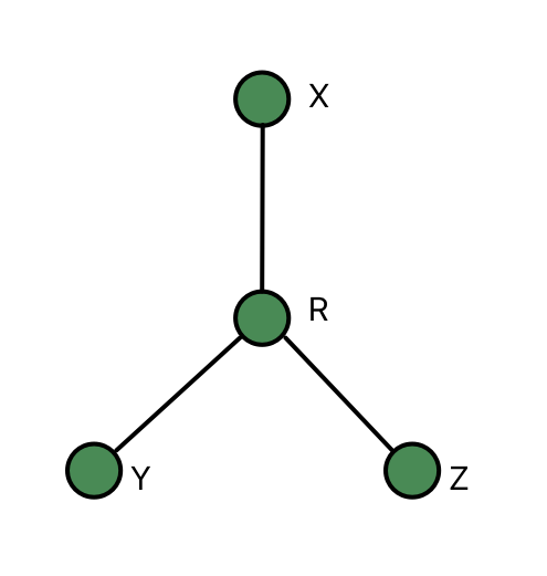
TreeRep is a recursive, divide and conquer algorithm. The first main idea (Lemma 1) is that for any metric on three points, we can construct a tree with four nodes such that . We will call such trees universal trees. The second main idea (Lemma 2) is that adding a fourth point to a universal tree can be done consistently and, more importantly, the additional point falls into one of seven different zones. Thus, TreeRep will first create a universal tree and then will sort the remaining data points into the seven different zones. We will then do recursion with each of the zones.
Lemma 1.
Given a metric on three points , there exists a (weighted) tree on four nodes , such that is adjacent to , the edge weights are given by , and , and the metric on the tree agrees with .
Definition 9.
The tree constructed in Lemma 1 is the universal tree on the three points . The additional node is known as a Steiner node.
An example of the universal tree can be seen in Figure 1(d). To understand the distinction between the seven different zones, we need to reinterpret Equation 2.1. We know that for any tree metric, and any four points , we have that
This inequality implies that the smaller two of the three numbers , and are equal. In this case, knowing which of the quantities are equal tells us the structure of the tree. Specifically, here will be the three points in our universal tree and will be the point that we want to sort. Then initially, we have four possibilities. The first possibility is that all three Gromov products are equal. This case will define its own zone. If this is not the case, then we have three possibilities depending on which two out of the three Gromov products are equal. Suppose we have that , then due to the triangle inequality, we have that . Thus, we will further subdivide this case into two more cases, depending on whether or . Each of these cases will define their own zone. Examples of the different cases can be seen in Figure 1. We can also see that there are two different types of zones. The first type is when we connect the new node directly to an existing node as seen in Figures 1(b) and 1(c). The second type is when we connect to an edge as seen in Figure 1(a). The formal definitions for the zones can be seen in Definition 13.
Lemma 2.
Let be a tree space. Let be four points in and let be the universal tree on with node as the Steiner node. Then we can extend to to include such that .
Definition 10.
Given a data set (consisting of data points, along with the distances amongst the points), a universal tree on (with as the Steiner node), let us define the following two zone types.
- 1.
The definition for zones of type one is split into the following two cases.
- (a)
- (b)
For a given permutation on ,
- (a)
- 2.
For a given permutation on ,
Using this terminology and our structural lemmas, we can describe a recursive algorithm that reconstructs the tree structure from a -hyperbolic metric. Given a data set we pick three random points and construct the universal tree . Then for all other , sort the ’s into their respective zones. Then for each of the seven zones we can recursively build new universal trees. For zones of type 1, pick any two points, and form the universal tree for (or ),. If there is only one node in this zone, connect it to (or ). For zones of type 2, pick any one point, and form the universal tree for . Note that during the recursive step for zones of type 2, we create universal trees with Steiner nodes as one of the nodes. Hence we need to compute the distance from to all other nodes sent to that zone. We can calculate this when we first place . Concretely, if is the Steiner node for the universal tree on , then for any , we will have that . The proof for the consistency of this formula is in the proof of Lemma 2.
Finally, to complete the analysis, the following lemma proves that we only need to check consistency of the metric within each zone to ensure global consistency.
Lemma 3.
Given a metric tree, and a universal tree on , we have the following
- 1.
If , then for all , we have that .
- 2.
If , then for all for , we have that .
TreeRep for General -Hyperbolic Metrics. Having seen the main geometric ideas behind TreeRep, we want to extend the algorithm to return an approximating tree for any given metric. For an arbitrary -hyperbolic metric, Lemma 2 does not hold. We can, however, modify it and leverage the intuition behind the original proof. Given four points , we do not satisfy one of the conditions of Lemma 2, if all three Gromov products have distinct values. Nevertheless, we can still compute the maximum of these three quantities. Furthermore, since we have a -hyperbolic metric, the smaller two products will be within of each other. Let us suppose that is the biggest. Then we place in if and only if or . Otherwise we place . Note that when we have tree metric, we have that if and only if .
As shown by Proposition 1, when we do this, we are introducing a distortion of at most between and . This suggests that when we do zone 2 recursive steps, we should pick the node that closest to as the third node for the universal tree. We see experimentally that this significantly improves the quality of the tree returned. Note, we do not have a global distortion bound for when the input is a general -hyperbolic metric. However, as we will see experimentally, we tend to produce trees with low distortion.
Proposition 1.
Given a -hyperbolic metric , the universal tree on and a fourth point , when sorting into its zone (), TreeRep introduces an additive distortion of at most between and .
Steiner nodes. A Steiner node is any node that did not exist in the original graph that one adds to it. We give a simple example to illustrate that Steiner nodes are necessary for reconstructing the correct tree. Additionally, we demonstrate that forming a graph and then computing any spanning tree (as done in [2, 16, 33]) will not recover the tree structure. Consider 3 points such that all pairwise distances are equal to . Then, the associated graph is a triangle and any spanning tree is a path. Then, the distance between the endpoints of the spanning tree is not correct; it has been distorted or stretched. The “correct” tree is obtained by adding a new node and connecting to , and making all the edge weights equal to . Thus, we need Steiner nodes when reconstructing the tree structure. Methods such as MST and LS [2] that do not add Steiner nodes will not produce the correct tree, when given a 0-hyperbolic metric, even though such algorithms do come with upper bounds on the distortion of the distances. In this setting, we want to obtain a tree that as accurately as possible represents the metric even at the cost of additional nodes; we do not simply want a tree that is a subgraph of a given graph.
4 Experiments
In this section, we demonstrate the effectiveness of TreeRep. Additional details about the experiments and algorithms can be found in Appendix 12.44 4 All code can be found at the following link https://github.com/rsonthal/TreeRep
For the first task of approximating metrics with tree metrics, we compare TreeRep against algorithms that find approximating trees; Minimum Spanning Trees (MST) [33], LevelTrees (LT) [11], Neighbor Join (NJ) [35], Low Stretch Trees (LS) [2, 16], ConstructTree (CT) [1], and ProbTree (BT) [3]. When comparing against such methods, we show that not only is TreeRep much faster than all of the above algorithms (except MST, and LS), but that TreeRep produces better quality metrics than MST, LS, LT, BT, and CT and metrics that are competitive with NJ. In addition to these methods, other methods such as UPGMA [39] also learn tree structures. However, these algorithms have other assumptions on the data. In particular, for UPGMA, the additional assumption is that the metric is an ultrametric. Hence we do not compare against such methods.
One important distinction between methods such as LS, MST, and LT and the rest, is that LS, MST, and LT require a graph as the input. This graph is crucial for these methods and hence sets these methods apart from the rest, as the rest only require a metric.
For the second task of learning hyperbolic embeddings, we compare TreeRep against Poincare Maps (PM) [30], Lorentz Maps (LM) [31], PT [36], and hMDS [36]. Since we can embed trees into with arbitrarily low distortion, we think of trees as hyperbolic representations. When comparing against such methods, we show that TreeRep is not only four to five orders of magnitude faster, but for low dimensions, and in many high dimensional cases, produces better quality embeddings.
We first perform a benchmark test for tree reconstruction from tree metrics. Then, for both tasks, we test the algorithms on three different types of data sets. First, we create synthetic data sets by sampling random points from . Second, we will take real world biological data sets that are believed to have hierarchical structure. Third, we consider metrics that come from real world unweighted graphs. In each case, we will show that TreeRep is an extremely fast algorithm that produces as good or better quality metrics. We will evaluate the methods on the basis of computational time, and the average distortion, as well as mean average precision (MAP) of the learned metrics.55 5 MAP is used in [30, 31, 36], while average distortion is used in [36]. The definitions are in the appendix.
Remark 2.
TreeRep is a randomized algorithm, so all numbers reported are averaged over 20 runs. The best number produced by TreeRep can be found in the Appendix.
Tree Reconstruction Experiments. Before experimenting with general -hyperbolic metrics, we benchmark our method on -hyperbolic metrics. To do this, we generate random synthetic -hyperbolic metrics. More details can be found in Appendix 12. Since TreeRep and NJ are the only algorithms that are theoretically guaranteed to return a tree that is consistent with the original metric, we will run this experiment with these two algorithms only. We compare the two algorithms based on their running times and the number of nodes in the trees. As we can see from Table 1, TreeRep is a much more viable algorithm at large scales. Additionally, the trees returned by NJ have double the number of nodes as the original trees. Contrarily, the trees returned by TreeRep have exactly the same number of nodes as the original trees.
| n | 11 | 40 | 89 | 191 | 362 | 817 | 1611 |
|---|---|---|---|---|---|---|---|
| TR | 0.053 | 0.23 | 0.0017 | 0.0039 | 0.02 | 0.08 | 0.12 |
| NJ | 0.084 | 0.0016 | 0.0067 | 0.036 | 0.18 | 1.7 | 15 |


| TR | NJ | MST | LS | CT | PT | LM | hMDS | hMDS-2 | |
|---|---|---|---|---|---|---|---|---|---|
| Time | 0.002 | 0.06 | 0.0001 | 0.002 | 0.076 | 312 | 971 | 11.7 | 0.008 |
Random points on Hyperbolic Manifold. We generate two different types of data sets. First, we hold the dimension constant and scale the coordinates. Second, we hold the magnitude of the coordinates constant and increase the dimension . Note these metrics do not come with an underlying graph! Hence to even apply methods such as MST, or LS we need to do some work. Hence, we create two different weighted graphs; a complete graph and a nearest neighbor graph.
For both types of data, Figures 2(a) and 2(b) show that as the scale and the dimension increase, the quality of the trees produced by TreeRep and NJ get better. Contrastingly, the quality of the trees produced by MST, ConstructTree, and LS do not improve. Hence we see that when we do not have an underlying sparse graph that was used to generate the metric, methods such as MST and LS do not perform well. In fact, they have the worst performance. This greater generality of possible inputs is one of the major advantages of our method. Thus, demonstrating that TreeRep is an extremely fast algorithm that produces good quality trees that approximate hyperbolic metrics. Furthermore, Table 2 shows that TreeRep is a much faster algorithm than NJ.
For the second task of finding hyperbolic embeddings, we compare against LM, PT and hMDS. For both LM, PT, and hMDS, we compute an embedding into , where is dimension of the manifold the data was sampled from. We also use hMDS to embed into , we call this hMDS-2. We can see from Figures 2(a) and 2(b) that TreeRep produces much better embeddings than LM, PT, and hMDS-2. Furthermore, LM and PT are extremely slow, with PT and LM taking 312 and 917 seconds on average, respectively. Thus, showing that TreeRep is 5 orders of magnitude faster than LM and PT, and produces better quality representations. On the other hand, since our points come from if we try embedding into with hMDS we should theoretically have zero error. However, these are high dimensional representations. We want low dimensional hyperbolic representations. Thus, we compared against hMDS-2 which did not perform well.


| Zeisel | CBMC | ||||||||||
|---|---|---|---|---|---|---|---|---|---|---|---|
| TR | NJ | MST | LS | CT | PT | PM | TR | NJ | MST | LS | |
| Time | 0.36 | 122.2 | 0.11 | 7.2 | >14400 | 8507 | 12342 | 2.8 | >14400 | 0.55 | 30 |
| Distortion | 0.117 | 0.144 | 0.365 | 0.250 | n/a | 0.531 | 0.294 | 0.260 | n/a | 1.09 | 1.45 |
Biological Data: scRNA seq and phylogenetic data. We also test on three real world biological data sets. The first data set consists of immunological distances from Sarich 1969. Given these distances, the goal is to recover the hierarchical phylogenetic structure. As seen in Figure 3, the trees returned by TreeRep and NJ recover this structure well, with sea lion and seal close to each other, and monkey and cat far away from everything else. Divergently, the trees and embeddings produced by MST, LS, ConstructTree, PM, and PT make less sense as phylogenetic trees.
The second type of data sets are the Zeisel and CBMC sc RNA-seq data set [44, 40]. These data sets are expected to be a tree as demonstrated in Dumitrascu et al. 2019. Here we used the various algorithms to learn a tree structure on the data or to learn an embedding into . The time taken and the average distortion are reported in Table 3. In this case, we see that TreeRep has the lowest distortion. Additionally, TreeRep is 20 times faster than NJ and is 20,000 to 40,000 times faster than PT and PM. Furthermore, NJ, CT, PT, and PM timed out (took greater than 4 hours) on the CBMC data set. For the CBMC data set, we see that TreeRep is only algorithm that produces good quality embeddings in a reasonable time frame. Again we see that if the input is a metric instead of a graph, algorithms such as MST and LS do not do well. We also tried to use hMDS for this experiment, but it either didn’t output a metric or it outputted the all zero metric.
| Graph | TR | NJ | MST | LT | CT | LS | PT | PT | PM | LM | LM | PM | |
|---|---|---|---|---|---|---|---|---|---|---|---|---|---|
| 2 | 200 | 2 | 2 | 200 | 200 | ||||||||
| MAP | |||||||||||||
| Celegan | 452 | 0.473 | 0.713 | 0.337 | 0.272 | 0.447 | 0.313 | 0.098 | 0.857 | 0.479 | 0.466 | 0.646 | 0.662 |
| Dieseasome | 516 | 0.895 | 0.962 | 0.789 | 0.725 | 0.815 | 0.785 | 0.392 | 0.868 | 0.799 | 0.781 | 0.874 | 0.886 |
| CS Phd | 1025 | 0.979 | 0.993 | 0.991 | 0.964 | 0.807 | 0.991 | 0.190 | 0.556 | 0.537 | 0.537 | 0.593 | 0.593 |
| Yeast | 1458 | 0.815 | 0.892 | 0.871 | 0.742 | 0.859 | 0.873 | 0.235 | 0.658 | 0.522 | 0.513 | 0.641 | 0.643 |
| Grid-worm | 3337 | 0.707 | 0.800 | 0.768 | 0.657 | - | 0.766 | - | - | 0.334 | 0.306 | 0.558 | 0.553 |
| GRQC | 4158 | 0.685 | 0.862 | 0.686 | 0.480 | - | 0.684 | - | - | 0.589 | 0.603 | 0.783 | 0.784 |
| Enron | 33695 | 0.570 | - | 0.524 | - | - | 0.523 | - | - | - | - | - | - |
| Wordnet | 74374 | 0.984 | - | 0.989 | - | - | 0.989 | - | - | - | - | - | - |
| Average Distortion | |||||||||||||
| Celegan | 2024 | 0.197 | 0.124 | 0.255 | 0.166 | 0.325 | 0.353 | 0.236 | 0.096 | 0.236 | 0.249 | 0.224 | 0.211 |
| Dieseasome | 1188 | 0.188 | 0.161 | 0.161 | 0.157 | 0.315 | 0.228 | 0.227 | 0.05 | 0.323 | 0.328 | 0.335 | 0.332 |
| CS Phd | 1043 | 0.204 | 0.134 | 0.298 | 0.161 | 0.282 | 0.291 | 0.295 | 0.105 | 0.374 | 0.378 | 0.378 | 0.380 |
| Yeast | 1948 | 0.205 | 0.149 | 0.243 | 0.243 | 0.282 | 0.243 | 0.230 | 0.089 | 0.246 | 0.248 | 0.234 | 0.234 |
| Grid-worm | 6421 | 0.188 | 0.135 | 0.171 | 0.202 | - | 0.234 | - | - | 0.196 | 0.203 | 0.192 | 0.193 |
| GRQC | 13422 | 0.192 | 0.200 | 0.275 | 0.267 | - | 0.206 | - | - | 0.212 | 0.198 | 0.193 | 0.193 |
| Enron | 180810 | 0.453 | - | 0.607 | - | - | 0.562 | - | - | - | - | - | - |
| Wordnet | 75834 | 0.131 | - | 0.336 | - | - | 0.071 | - | - | - | - | - | - |
| Time in seconds | |||||||||||||
| Celegan | 0.21 | 0.014 | 0.28 | 0.0002 | 0.086 | 0.9 | 0.001 | 573 | 1156 | 712 | 523 | 1578 | 1927 |
| Dieseasome | 0.17 | 0.017 | 0.41 | 0.0003 | 0.39 | 15.76 | 0.001 | 678 | 1479 | 414 | 365 | 978 | 1112 |
| CS Phd | 0.23 | 0.037 | 2.94 | 0.0007 | 1.97 | 226 | 0.006 | 1607 | 4145 | 467 | 324 | 768 | 1149 |
| Yeast | 0.057 | 8.04 | 0.0008 | 8.21 | 957 | 0.001 | 9526 | 17876 | 972 | 619 | 1334 | 2269 | |
| Grid-worm | 0.731 | 163 | 0.001 | 191 | - | 0.007 | - | - | 2645 | 1973 | 4674 | 5593 | |
| GRQC | 0.42 | 311 | 0.0014 | 70.9 | - | 0.006 | - | - | 7524 | 7217 | 9767 | 1187 | |
| Enron | - | 27 | - | 0.013 | - | - | 0.13 | - | - | - | - | - | - |
| Wordnet | - | 74 | - | 0.18 | - | - | 0.08 | - | - | - | - | - | - |
Unweighted Graphs. Finally, we consider metrics that come from unweighted graphs. We use eight well known graph data sets from [34]. Table 7 records the performance of all the algorithms for each of these data sets. For learning tree metrics to approximate general metrics, we see that NJ has the best MAP, with TreeRep, MST, and LS tied for second place. In terms of distortion, NJ is the best, TreeRep is second, while MST is third and LS is sixth. However, NJ is extremely slow and is not viable at scale. Hence, in this case, we have three algorithms with good performance at large scale; TreeRep, MST, and LS. However, MST and LS did not perform well in the previous experiments.
For the task of learning hyperbolic representations, we see that PM, LM, and PT are much slower than the methods that learn a tree first. In fact, these algorithms were too slow to compute the hyperbolic embeddings for the larger data sets. Additionally, this extra computational effort does not always result in improved quality. In all cases, except for the Celegan data set, the MAP returned by TreeRep is superior to the MAP of the -dimensional embeddings produced by PM, LM, and PT. In fact, in most cases, these 2-dimensional embeddings, have worse MAP than all of the tree first methods. Even when they learn 200-dimensional embeddings, PM, LM and PT have worse MAP than TreeRep on most of the data sets. Furthermore, except for PT200, the average distortion of the metric returned by TreeRep is superior to PT2, PM, an LM. Thus, showing the effectiveness of TreeRep at learning good Hyperbolic representations quickly.
5 Broader Impact
There are multiple aspects to the broader impacts of our work, from the impact upon computational biology, specifically, to the impact upon data sciences more generally. The potential impacts on society, both positive and negative, are large. Computational biology is undergoing a revolution due to simultaneous advances in the creation of novel technologies for the collection of multiple and novel sources of data, and in the progress of the development of machine learning algorithms for the analysis of such data. Social science has a similar revolution in its use of computational techniques for the analysis and gathering of data.
Cellular differentiation is the process by which cells transition from one cell type (typically an immature cell) into more specialized types. Understanding how cells differentiate is a critical problem in modern developmental and cancer biology. Single-cell measurement technologies, such as single-cell RNA-sequencing (scRNA-seq) and mass cytometry, have enabled the study of these processes. To visualize, cluster, and infer temporal properties of the developmental trajectory, many researchers have developed algorithms that leverage hierarchical representations of single cell data. To discover these geometric relationships, many state-of-the-art methods rely on distances in low-dimensional Euclidean embeddings of cell measurements. This approach is limited, however, because these types of embeddings lead to substantial distortions in the visualization, clustering, and the identification of cell type lineages. Our work is specifically focused on extracting and representing hierarchical information.
On the more negative side, these algorithms might also be used to analyze social hierarchies and to divine social structure from data about peoples’ interactions. Such tools might encourage, even justify, the intrusive and pervasive collection of data about how people interact and with whom.
References
- Abraham et al. [2007] Ittai Abraham, Mahesh Balakrishnan, Fabian Kuhn, Dahlia Malkhi, Venugopalan Ramasubramanian, and Kunal Talwar. Reconstructing Approximate Tree Metrics. In Proceedings of the Twenty-sixth Annual ACM Symposium on Principles of Distributed Computing, PODC ’07, pages 43–52, New York, NY, USA, 2007. ACM.
- Alon et al. [1995] Noga Alon, Richard M. Karp, David Peleg, and Douglas West. A graph-theoretic game and its application to the -server problem. SIAM J. Comput., 24(1):78–100, February 1995. ISSN 0097-5397. doi: 10.1137/S0097539792224474. URL https://doi.org/10.1137/S0097539792224474.
- Bartal [1998] Yair Bartal. On Approximating Arbitrary Metrics by Tree Metrics. In Proceedings of the Thirtieth Annual ACM Symposium on Theory of Computing, STOC ’98, pages 161–168, New York, NY, USA, 1998. ACM. ISBN 0-89791-962-9.
- Bermudo et al. [2013] Sergio Bermudo, José M. Rodríguez, José M. Sigarreta, and Jean-Marie Vilaire. Gromov Hyperbolic Graphs. Discrete Mathematics, 313(15):1575 – 1585, 2013.
- Blasius et al. [2018] T. Blasius, T. Friedrich, A. Krohmer, and S. Laue. Efficient Embedding of Scale-Free Graphs in the Hyperbolic Plane. IEEE/ACM Transactions on Networking, 26(2):920–933, April 2018.
- Bonk and Schramm [2000] M. Bonk and O. Schramm. Embeddings of Gromov Hyperbolic Spaces. Geometric & Functional Analysis GAFA, 10(2):266–306, Jun 2000.
- Bridson and Häfliger [2013] M.R. Bridson and A. Häfliger. Metric Spaces of Non-Positive Curvature. Grundlehren der mathematischen Wissenschaften. Springer Berlin Heidelberg, 2013. ISBN 9783662124949.
- Campbell [2013] L. Campbell. Historical Linguistics: An Introduction. Edinburgh University Press, 2013. ISBN 9780748675609.
- Carnahan [2010] S. Carnahan. It is Well Known that Hyperbolic Space is -Hyperbolic, but what is Delta? MathOverflow, 2010. URL https://mathoverflow.net/q/23064.
- Chepoi and Dragan [2000] Victor Chepoi and Feodor Dragan. A Note on Distance Approximating Trees in Graphs. European Journal of Combinatorics, 21(6):761 – 766, 2000.
- Chepoi et al. [2008] Victor Chepoi, Feodor Dragan, Bertrand Estellon, Michel Habib, and Yann Vaxès. Diameters, Centers, and Approximating Trees of -Hyperbolic Geodesic Spaces and Graphs. In Proceedings of the Twenty-fourth Annual Symposium on Computational Geometry, SCG ’08, pages 59–68, New York, NY, USA, 2008. ACM.
- Cvetkovski and Crovella [2016] Andrej Cvetkovski and Mark Crovella. Multidimensional Scaling in the Poincaré Disk. Applied Mathematics and Information Sciences, 10:125–133, 01 2016.
- Dhingra et al. [2018] Bhuwan Dhingra, Christopher J. Shallue, Mohammad Norouzi, Andrew M. Dai, and George E. Dahl. Embedding Text in Hyperbolic Spaces, 2018.
- Dumitrascu et al. [2019] Bianca Dumitrascu, Soledad Villar, Dustin G. Mixon, and Barbara E. Engelhardt. Optimal Marker Gene Selection for Cell Type Discrimination in Single Cell Analyses. bioRxiv, 2019.
- Dyubina and Polterovich [2001] ANNA Dyubina and IOSIF Polterovich. Explicit Constructions of Universal -Trees and Asymptotic Geometry of Hyperbolic Spaces. Bulletin of the London Mathematical Society, 33(6):727?734, Nov 2001.
- Elkin et al. [2005] Michael Elkin, Yuval Emek, Daniel A. Spielman, and Shang-Hua Teng. Lower-stretch spanning trees. In Proceedings of the Thirty-Seventh Annual ACM Symposium on Theory of Computing, STOC ’05, page 494–503, New York, NY, USA, 2005. Association for Computing Machinery. ISBN 1581139608. doi: 10.1145/1060590.1060665. URL https://doi.org/10.1145/1060590.1060665.
- Ganea et al. [2018] Octavian Ganea, Gary Becigneul, and Thomas Hofmann. Hyperbolic Neural Networks. In Advances in Neural Information Processing Systems 31, pages 5345–5355. Curran Associates, Inc., 2018.
- Gilbert and Sonthalia [2020] Anna C. Gilbert and Rishi Sonthalia. Project and Forget: Solving Large Scale Metric Constrained Problems, 2020. URL https://openreview.net/forum?id=SJeX2aVFwH.
- Graham and Winkler [1985] R. L. Graham and P. M. Winkler. On Isometric Embeddings of Graphs. Trans. Amer. Math. Soc., 288(2):527–536, 1985. ISSN 0002-9947.
- Gromov [1987] M. Gromov. Hyperbolic Groups, pages 75–263. Springer New York, New York, NY, 1987.
- Gulcehre et al. [2019] Caglar Gulcehre, Misha Denil, Mateusz Malinowski, Ali Razavi, Razvan Pascanu, Karl Moritz Hermann, Peter Battaglia, Victor Bapst, David Raposo, Adam Santoro, and Nando de Freitas. Hyperbolic Attention Networks. In International Conference on Learning Representations, 2019.
- Hamann [2018] MATTHIAS Hamann. On the Tree-Likeness of Hyperbolic Spaces. Mathematical Proceedings of the Cambridge Philosophical Society, 164(2):345–361, 2018. doi: 10.1017/S0305004117000238.
- Jahren [2012] Bjorn Jahren. Geometric Structures in Dimension Two, 2012. URL http://www.uio.no/˜studier/emner/matnat/math/MAT4510/h13/gs.pdf.
- Johnson and Lindenstrauss [1984] William B. Johnson and Joram Lindenstrauss. Extensions of Lipschitz mappings into a Hilbert space. In Conference in modern analysis and probability (New Haven, Conn., 1982), volume 26 of Contemp. Math., pages 189–206. Amer. Math. Soc., Providence, RI, 1984.
- Khrulkov et al. [2019] Valentin Khrulkov, Leyla Mirvakhabova, Evgeniya Ustinova, Ivan Oseledets, and Victor Lempitsky. Hyperbolic Image Embeddings, 2019.
- Klimovskaia et al. [2019] Anna Klimovskaia, David Lopez-Paz, Léon Bottou, and Maximilian Nickel. Poincaré Maps for Analyzing complex Hierarchies in Single-Cell Data. bioRxiv, 2019. doi: 10.1101/689547.
- Krioukov et al. [2010] Dmitri Krioukov, Fragkiskos Papadopoulos, Maksim Kitsak, Amin Vahdat, and Marián Boguñá. Hyperbolic Geometry of Complex Networks. Physical Review E, 82(3), Sep 2010. ISSN 1550-2376. doi: 10.1103/physreve.82.036106. URL http://dx.doi.org/10.1103/PhysRevE.82.036106.
- Linial [2002] Nathan Linial. Finite Metric Spaces: Combinatorics, Geometry and Algorithms. In Proceedings of the Eighteenth Annual Symposium on Computational Geometry, SCG ’02, pages 63–63, New York, NY, USA, 2002. ACM.
- Linial et al. [1995] Nathan Linial, Eran London, and Yuri Rabinovich. The Geometry of Graphs and Some of its Algorithmic Applications. Combinatorica, 15(2):215–245, Jun 1995.
- Nickel and Kiela [2017] Maximilian Nickel and Douwe Kiela. Poincaré Embeddings for Learning Hierarchical Representations. In NIPS, 2017.
- Nickel and Kiela [2018] Maximilian Nickel and Douwe Kiela. Learning Continuous Hierarchies in the Lorentz Model of Hyperbolic Geometry. In ICML, 2018.
- Peleg and Ullman [1989] David. Peleg and Jeffrey D. Ullman. An Optimal Synchronizer for the Hypercube. SIAM Journal on Computing, 18(4):740–747, 1989.
- Prim [1957] R. C. Prim. Shortest Connection Networks and Some Generalizations. The Bell System Technical Journal, 36(6):1389–1401, Nov 1957.
- Rossi and Ahmed [2015] Ryan A. Rossi and Nesreen K. Ahmed. The network data repository with interactive graph analytics and visualization. In AAAI, 2015. URL http://networkrepository.com.
- Saitou and Nei [1987] Naruya Saitou and Masatoshi Nei. The Neighbor-joining Method: A New Method for Reconstructing Phylogenetic Trees. Molecular biology and evolution, 4 4:406–25, 1987.
- Sala et al. [2018] Frederic Sala, Chris De Sa, Albert Gu, and Christopher Re. Representation Tradeoffs for Hyperbolic Embeddings. Proceedings of the 35th International Conference on Machine Learning, pages 4460–4469, July 2018.
- Sarich [1969] Vincent M. Sarich. Pinniped Phylogeny. Systematic Biology, 18(4):416–422, 12 1969.
- Sarkar [2012] Rik Sarkar. Low Distortion Delaunay Embedding of Trees in Hyperbolic Plane. In Proceedings of the 19th International Conference on Graph Drawing, GD’11, pages 355–366, Berlin, Heidelberg, 2012. Springer-Verlag.
- Sokal et al. [1958] R.R. Sokal, C.D. Michener, and University of Kansas. A Statistical Method for Evaluating Systematic Relationships. University of Kansas science bulletin. University of Kansas, 1958.
- Stoeckius et al. [2017] Marlon Stoeckius, Christoph Hafemeister, William Stephenson, Brian Houck-Loomis, Pratip K Chattopadhyay, Harold Swerdlow, Rahul Satija, and Peter Smibert. Simultaneous epitope and transcriptome measurement in single cells. Nature Methods, 14(9):865–868, 2017. doi: 10.1038/nmeth.4380.
- Verbeek and Suri [2016] Kevin Verbeek and Subhash Suri. Metric Embedding, Hyperbolic Space, and Social Networks. Computational Geometry, 59:1 – 12, 2016.
- Young [2008] Robert Young. Notes on Asymptotic Cones, 2008. URL http://pi.math.cornell.edu/˜riley/Conferences/SL(n,Z)/Young_on_Asymptotic_Cones.pdf.
- Yu and De Sa [2019] Tao Yu and Christopher M De Sa. Numerically Accurate Hyperbolic Embeddings Using Tiling-Based Models. In Advances in Neural Information Processing Systems 32, pages 2021–2031. Curran Associates, Inc., 2019.
- Zeisel et al. [2015] Amit Zeisel, Ana B. Muñoz-Manchado, Simone Codeluppi, Peter Lönnerberg, Gioele La Manno, Anna Juréus, Sueli Marques, Hermany Munguba, Liqun He, Christer Betsholtz, Charlotte Rolny, Gonçalo Castelo-Branco, Jens Hjerling-Leffler, and Sten Linnarsson. Cell Types in the Mouse Cortex and Hippocampus Revealed by Single-cell rna-seq. Science, 347(6226):1138–1142, 2015.
6 Metric First Discussion and Justification
Table 7 shows that for most of the data sets, learning a tree structure first and then embedding it into hyperbolic space, yields embeddings with better MAP and average distortion compared to methods that learn the embedding directly. One possible explanation for this phenomenon is that the optimization problems that seek the embeddings directly are not being solved optimally. That is, the algorithms get stuck at some local minimum. Another possibility is that there is a disconnect between the objective being optimized and the statistics calculated to judge the quality of the embeddings.
We propose that there are geometric facts about hyperbolic space that suggest embedding by first learning a tree is the correct approach. The tree-likeness of hyperbolic space has been studied from many different approaches. We present details from Hamann 2018, Dyubina and Polterovich 2001 and looks at the geometry of at its two extremes; large scale and small scale. Since is a manifold, we know that at small scales hyperbolic space looks like Euclidean space. Additionally, in the Poincare disk, the hyperbolic Riemannian metric is given by and is just a re-scaling of the Euclidean metric. Thus, at small scales, hyperbolic space is similar to Euclidean space.
Hence to take advantage of hyperbolic representations (i.e., why learn a hyperbolic representation instead of a Euclidean one), we want to embed data into at scale. To study the large scale geometry of , we consider the asymptotic cone for hyperbolic space . In particular, we can think of the asymptotic cone as the “view of our space from infinitely far away”. See the more detailed discussion in Appendix 8 for examples and complete definitions. The following connects to -tree spaces.
Theorem 2.
[42] is a complete -tree.
Thus, we see that the large scale structure of hyperbolic space is a tree, indicating a strong connection between learning trees and learning hyperbolic embeddings. Furthermore, it can be shown that is a -universal tree. That is, any tree with finitely many nodes can be embedded into exactly. However, these are still embeddings into . We would like to study embeddings into .
Definition 11.
A metric space admits an isometric embedding at infinity into the space if there exists a sequence of positive scaling factors such that for every point , there exists an infinite sequence of points in such that for all
Theorem 3.
[15] can be isometrically embedded at infinity into .
Thus, we can embed any tree into with arbitrarily low distortion. A type of converse is also true.
Definition 12.
A (geodesic) ray is a (isometric) homeomorphic image of , such that for any ball of finite diameter, lies outside eventually.
Hamann 2018 showed that we can construct a rooted -tree inside , such that every geodesic ray in eventually converges to a ray of . Thus, showing that any configuration of points at scale in can be approximated by a tree. Additionally, larger the scale points can be better approximated by trees. More details can be found in Appendix 9. Thus, showing that learning a tree and then embedding this tree into is equivalent to learning hyperbolic representations at scale.
This provides an explanation for why as the scale and dimension increased, TreeRep found a tree that better approximated the hyperbolic metric in Section 4. This also provides a justification for why learning a tree first, results in better hyperbolic representations.
7 Proofs
7.1 Tree Representation Proofs
Lemma 1. Given a metric on three points , there exists a (weighted) tree on four nodes , such that is adjacent to , the edge weights are given by , and , and the metric on the tree agrees with .
Proof.
The basic structure of this tree can be seen in Figure 1(d). To prove that the metrics agree we such need to see the following calculation.
Here is the metric on the tree . ∎
One important fact that we need is that if is a metric graph, then for any three distinct points , the geodesics connecting them intersect at a unique point. As seen in Lemma 1, we refer to this point a Steiner point . It is now important to note that even though may not be a point in the data set we are given, but [7]. Thus, in the following lemmas, whenever we find a Steiner point, we will assume that the metric is defined on .
Lemma 4.
If is a tree metric and are three points then
- 1.
if and only if
- 2.
if and only if .
- 3.
if and only if .
Here is the unique path connecting and .
Proof.
For 1. we see that
Thus we have that .
For 2. we see that
The proof for 3 is similar to that of 2.
∎
Lemma 2. Let be a tree space. Let be four points in and let be the universal tree on with node as the Steiner node. Then we can extend to to include such that .
Proof.
We note that there are four different possible cases for the configuration of depending on the relationship amongst the Gromov products. Each case determines a different placement of , as follows:
- 1.
If , then replace with to obtain .
- 2.
If , then connect to via an edge of weight to obtain .
- 3.
If there exists a permutation such that,
and , then connect to via an edge of weight to obtain .
- 4.
If there exists a permutation such that,
and , then add a Steiner point on the edge with and connect to via an edge of weight to obtain .
To prove that these extensions of are consistent, first let us prove that there are exactly four cases. To do that, first note that since we have a -hyperbolic metric, at least two of the three Gromov products must be equal. Using the triangle inequality, we can see that for any three points the following holds
That is, either we are in the first two cases and three of products are equal, or we have that two of the products are equal. In the case that two of the products are equal, the permutation tells us which of the two are equal and we further subdivide into the case whether or as we cannot have .
Therefore, there are at most four possible configuration cases and it remains to show that the new tree is consistent with on the four points. In each case, we present the high level intuition for why these modification result in a consistent tree. The low level details about the metric numbers can easily be checked.
Case 1: If , then we replaced with in . In this case, using Lemma 4, we see that must lie on all tree geodesics . Since the metric comes from a tree, these three geodesics can only intersect at one point . Thus, we must replace with .
To see that the metric is consistent, we need to verify that = . To see we have the following:
Case 2: If
then we can see that . In this case, lies on geodesics , , , , , . Thus, we must have a star shaped graph with in the center.
To see that the metric is consistent we just need to verify that . To see that we have the following calculation.
Case 3: In this case suppose condition 4 is true. Without loss of generality assume that is the identity map. In each case, we have a tree that looks like a tree in Figure 1. In this case, we can do the calculations and see that . That is, the geodesics all intersect at the same point. Thus, again telling us our tree structure.
To check that the metric is consistent, we need to verify that . Before we can do that, let us first verify that
To verify this we need to the following calculation
We then can see that
Note and the consistency of the metric implies that . Finally, we can see as follows.
Note that this also implies that .
Case 4: In this case, suppose condition 3 is true. Without loss of generality assume that is the identity map. Then in this case, we still have that , but in addition we have that . Thus, again telling us our tree structure.
In this case, to verify that the metric is consistent, we need to check that . To see this we have the following calculations.
Thus, now it suffices to show that , which can be seen using the following calculations.
This also implies that . ∎
The proof of Lemma 2 shows that there are a number of ways to extend to include the new point . To clarify our discussion of the extension of , we introduce new terminology.
Definition 13.
Given a data set (consisting of data points, along with the distances amongst the points), a universal tree on (with as the Steiner node), let us defining the following three zone types. The first type is associated only with the Steiner node , while the other two types are defined for each of the original nodes .
- 1.
- 2.
- 3.
Note that there are seven zones total.
Lemma 5.
Let is a metric tree. Let and let if and only if has at least two disconnected components and are in distinct components.
Proof.
Suppose . In metric trees, we know that there exist unique simple path between any two points. Therefore, if, after removing , a path connecting remained (i.e., they are in the same component), then there are two simple paths connecting in , which is not possible.
Suppose are in two separate components of , then because is path connected, the geodesic between and must pass through . ∎
Lemma 3. Given a metric tree, and a universal tree on , we have the following
- 1.
If , then for all , we have that .
- 2.
If , then for all for , then we have that .
Proof.
First let us prove statement 1. To do this, let us analyze the possible zones to which belongs.
Case 1: Suppose (similar for ). Then we have that . This, implies that . Thus, by Lemma 4, we have that . Similarly we have that .
Now since , we know that . Similarly, know that . Then using Lemma 5, on removing , we see that and are different connected components. Then since , we see that is in one connected component. Thus, are in different components. Thus, by Lemma 5.
Case 2: Suppose (similar for ). Now let be the Steiner node of the universal tree on . In this case we know from Lemma 2 that and that .
Now since , we know that . Similarly, know that . Then using Lemma 5, on removing , we see that and are different connected components. Then since , we see that is in one connected component. Thus, are in different components. Thus, by Lemma 5.
Case 3: . Let be the Steiner node for the universal tree on . Now my Lemma 2, we know that . Thus, again by removing and using Lemma 5, and are in different. We also have that by Lemma 2 . Thus are in the same connected component of . Thus, and are in different connected components. Thus, by Lemma 5,
Thus in all cases, we can see that
Now let us prove statement 2. Without loss of generality assume that
for . Then from Lemma 2, we know that and , but . Thus, using Lemma 5 on removing , and and in different components and is in the same component as and is in the same component as . Thus, again using Lemma 5, we have that .
∎
Theorem 1. Given , a -hyperbolic metric space, and points , TreeRep returns a tree . In the case that , , and has the fewest possible nodes. TreeRep has worst case run time . Furthermore the algorithm is embarrassingly parallelizable.
Proof.
The proof of this theorem follows directly from our structural lemmas. More precisely, we show that for , TreeRep returns a consistent metric via induction on , the number of data points.
Inductive Hypothesis: Assume that for all , our data set of points is consistent with a -hyperbolic metric , then TreeRep returns a tree that is consistent with on the points.
Inductive Step: Assume that is the last vertex attached to . By the inductive hypothesis, we know that without , is consistent on with so we only need to show that it is consistent with the addition of .
Now let be the universal tree used to sort in the penultimate recursive step. Let be the Steiner node. Then by Lemma 2, we know that , , and .
Now without loss of generality assume that was sorted in a zone for . That is, for .
Case 1: If . Then from Lemma 1, we know that for all , we have that . Thus, having and is sufficient to show consistency.
Now, since was placed last there is at most one other point in , and due to Lemma 1.
Case 2: If . Then from Lemma 2, we know that for all , for we have that . Thus, having and is sufficient to show consistency.
Suppose . Then from Lemma 1, we have that . Thus, having and is sufficient to show consistency.
Finally, since was the last node placed there are no other nodes in .
Thus, we have the the tree returned by TreeRep is consistent with the input metric .
Notice that whenever we add a Steiner node we fix the position of at least one data point node. We then look at Gromov inner products. Thus, we have a worst case running time of .
Additionally, the part where we place nodes into their respective zones can be done in parallel. Thus, if we have threads then the running time is for the worst running times.
The final part of the theorem is that we return the tree with the smallest possible nodes. Whenever we look at any triangle formed by three points , we place a Steiner node . Now, if none of the distances from to is 0, then this Steiner node must exist in all tree consistent with . If one of these distances is 0, we contracted that edge and got rid of . Thus, along with the local consistency argument above this shows that all Steiner nodes that we have placed are necessary (the local consistency argument implies that no two of the Steiner nodes placed could in fact be made into one node due to the nodes beings in different regions). Thus, we have the fewest possible nodes.
∎
7.2 Tree Approximation Proofs
Proposition 1. Given a -hyperbolic metric , the universal tree on and a fourth point , when sorting into its zone , TreeRep introduces an additive distortion of between and
Proof.
Without loss of generality assume that is the identity. In this case, we know that , and that . Thus, we have the following:
∎
8 Geometry: Asymptotic Cones
Definition 14.
An ultrafilter on is a subset of such that
- 1.
If and then
- 2.
then
- 3.
For any , exactly of is in
- 4.
.
One way to view is as defining a probability measure on . In particular, we will view the sets in to be large and the sets not in to be small. Hence, we can define a measure such that for all we have that and for all we have that .
In this way, we can see that is a finitely additive measure on . One common method to define ultrafilters is to take a point and let be the set of all sets that contain . In this case, the measure has a point mass at and zero mass elsewhere. Such filters are known an principal ultrafilters.
Given a measure on , we can use it to define limits and convergence in . In particular, we have that a sequence converges to , if for all we have that
We will denote limits of this form as .
We will make use of ultrafilters to construct the asymptotic cone. We will do this via looking at a non-principal ultrafilter on . We consider non-principal ultrafilters as we want to get a view from infinity, and we do not want to be in the case when one particular index in has the entire mass. Hence we restrict ourselves to non-principal ultrafilters. One nice characterization of non-principal ultrafilters is that they are exactly the ultrafilters that have no finite sets.
Now that we have mathematical framework in which we can take limits, let us define our asymptotic cone. Let be a non-principal ultrafilter on . Let be a sequence of base points and let be a sequence of scaling factors that go to infinity. Let be the metric on our space . Then let
While this space looks huge we will define an equivalence relation and mod out by this relation to obtain better structure on this space. Given two points we say that if
We can now define our asymptotic cone . We can also define a metric on this space as follows, given
Let us look at a few examples to get a handle on what looks like.
- 1.
Example 1: Let us first consider . We know that is scale invariant. This results in being equivalent to . In fact, if we assume that , then the map is an isometry from to
- 2.
Example 2: Suppose is a bounded metric space. In this case is a single point.
Definition 15.
A metric space can be isometrically embedded into a metric space if there exists a map such that for all we have that
Such a map is known as an isometry.
Definition 16.
A metric space is homogenous if for all there exists an isometry such that .
Definition 17.
Given a -tree , the valency of a point in an -tree is the number of connected components in . Let the valence of a the tree, denoted , be the maximum valence of any point in .
Definition 18.
A -tree is a -universal if every -tree with can be isometrically embedded into .
Here we can see that we can embed any finite tree into a -universal tree . Hence, if could isometrically embed into then we can embed any tree into . This and more turns out to be true.
Theorem 4.
[15] Any -universal -tree can be isometrically embedded into the asymptotic cone for any complete simply connected manifold of negative curvature.
9 Geometry: Geodetic Tree
In general, it is rare to be able isometrically embed one space into another. Hence, we have the following weaker definition.
Definition 19.
We say that we can quasi isometrically embed a metric space into a metric space if there exists a map and real numbers such that , and for all we have that
Such isometries are called -quasi-isometries.
It is has been shown that any -hyperbolic metric space with bounded growth admits a quasi-isometric embedding into [6].
Definition 20.
We say that a ray is quasi geodetic if instead of being an isometric image of , we have that is an quasi-isometric image of .
Definition 21.
A ray is eventually (quasi) geodetic if it has a subray that is (quasi) geodetic.
Theorem 5.
[22] For all , there is a constant , such that for every two points , every -quasi-geodesic between them lies in a -neighborhood around every geodesic between and and vice versa.
Definition 22.
Two geodetic rays are equivalent if for any sequence of points on , we have for an
Definition 23.
The boundary of is the equivalence class of all geodesic rays.
Theorem 6.
[22] There is an -tree such that the canonical map from to exists and has the following properties.
- 1.
It is surjective;
- 2.
there is a constant depending only on such that has at most elements for each .
Theorem 7.
The above two theorems tell us that given any geodesic ray in there is exists a ray in that is equivalent to (via in Definition 22). Furthermore this ray in is -quasi-geodetic ray in . Thus, due to Theorem 5 any configuration of points at scale in can be approximated by a tree such that the larger the scale, better the approximation.
10 TreeRep Best
So far all numbers for the TreeRep algorithm that we have reported are averages. But due to the speed of the algorithm, we can actually run the experiment multiple times and pick the tree with the best metric.
| No Opt | Heuristic Opt | Full Opt | ||||
|---|---|---|---|---|---|---|
| Graph | MAP | Distortion | MAP | Distortion | MAP | Distortion |
| Celegan | 0.508 | 0.173 | 0.539 | 0138 | 0.547 | 0.119 |
| Diseasome | 0.912 | 0.134 | 0.911 | 0.106 | 0.890 | 0.092 |
| CS PhD | 0.987 | 0.134 | 0.984 | 0.119 | 0.968 | 0.121 |
| Yeast | 0.841 | 0.171 | 0.833 | 0.150 | 0.808 | 0.135 |
| Grid-worm | 0.727 | 0.154 | 0.728 | 0.125 | - | - |
| GRQC | 0.699 | 0.175 | 0.694 | 0.152 | - | - |
11 Improving Distortion
We have seen that in the case of unweighted graphs TreeRep produces better MAP than PM, LM, and PT. However, PT tends to have better average distortion. Hence, we want to be able to improve the distortion. Once we have learned the tree structure we can set up an optimization problem to learn the edge weights on the tree to improve the distortion. Specifically, since the metric comes from the tree, for any pair of data points, there is exactly one path connecting the two data points. Thus, regardless of the edges weights, this path is the shortest path between the data points. Thus, we can set up an optimization problem of the following form:
Here is a vector containing the edge weights, is a vector containing the original metric, and is a matrix that encodes all of the paths. This optimization problem however, is unfeasible as gets longer. So instead we sample some rows of and solve a heuristic problem. As can be seen from Table 6, we are still faster than NJ but now have improved our distortion without sacrificing MAP.
| Graph | Time | Distortion | MAP | Distortion | MAP |
|---|---|---|---|---|---|
| TreeRep | MST | ||||
| Celegans | 0.69 | 0.157 | 0.504 | 0.195 | 0.357 |
| Diseasome | 1.56 | 0.121 | 0.891 | 0.111 | 0.774 |
| CS Phd | 1.2 | 0.152 | 0.971 | 0.170 | 0.989 |
| Yeast | 4.2 | 0.163 | 0.813 | 0.171 | 0.862 |
| Grid Worm | 32 | 0.164 | 0.707 | 0.151 | 0.768 |
| GRQC | 68 | 0.157 | 0.676 | 0.159 | 0.669 |
12 Experiment and Practical Details
12.1 MAP and Average Distortion
Definition 24.
Given two metrics on a finite set the average distortion is:
Smaller average distortion implies greater similarity between and .
In many cases, the metric learned by the various algorithms will be a scalar multiple of the actual metric, so we will solve for the scale , before calculating the average distortion.66 6 For NJ and LT, computing this made the average distortion worse, so we report numbers un-scaled. Additionally, computing is too computationally expensive for bigger data sets and was not done for the Enron and Wordnet data set.
Definition 25.
Let be a metric on the nodes of a graph . For , let be the neighborhood of . Then let . Then the mean average precision (MAP) is defined to be
Closer MAP is to 1, the closer is to approximating .
12.2 TreeRep
There are a few practical details that must be discussed in relation to the TreeRep algorithm.
- 1.
Pre-allocate the matrix for the weights of edges of the tree as a dense matrix. Doing this greatly speeds up computations. Note the proof of Lemma 2, show that we need at most Steiner nodes. Thus, the tree has about nodes. Since the input to the algorithm is a dense matrix, we already need memory. Thus, having a dense matrix is still linear memory usage in the size of the input.
- 2.
When doing zone 2 recursions pick the node closest to as the new as suggested by Proposition 1.
- 3.
The placement of nodes into their respective zones can be done in parallel. For all of the experiments in the paper, we used 8 threads to do the placement for all of the experiments, except that we used 1 thread for the random points from experiment and for CBMC experiment.
- 4.
All of the numbers reported are averages over 20 iterations. We could have also picked the best over 20 iterations as our algorithm is fast enough for this to be viable.
- 5.
When checking for equality, instead of checking for exact equality, we checked whether two numbers are within 0.1 of each other.
- 6.
It is possible for some of the edge weights to be set to a negative number. In this case, after the algorithm terminated we set those edge weights to 0.
12.3 Bartal
We sample 200 trees from the distribution and compute the metric assuming that we are embedding into the distribution restricted to these 200 trees.
12.4 Neighbor Join
The following implementation of NJ was used: http://crsl4.github.io/PhyloNetworks.jl/latest/. We set the options so as to not have any negative edge weights.
12.5 MST
Prim’s algorithm for calculating MST was used. We used the implementation at https://github.com/JuliaGraphs/LightGraphs.jl
12.6 LS
12.7 LevelTree and ConstructTree
To the best of the authors knowledge there does not exist a publicly available implementations of these algorithms. Both of these algorithms were implemented by the authors.
Note that LevelTree claims to be a algorithm, but this only true, once we have calculated the sphere needed for the algorithm. However, it takes time to calculate the spheres (equivalent to solving single source all destination shortest path problem).
12.8 PM and LM
The following options were used. The number of epochs was to set to be higher than default. Everything else was left at default. One note about PM and LM is that their objective function is set up to optimize for MAP and not average distortion.
- 1.
-lr 0.3
- 2.
-epochs 1000
- 3.
-burnin 20
- 4.
-negs 50
- 5.
-fresh
- 6.
-sparse
- 7.
-train_threads 2
- 8.
-ndproc 4
- 9.
-batchsize 10
For PM we used -manifold poincare, for LM we used -manifold lorentz. The code is taken from https://github.com/facebookresearch/poincare-embeddings
12.9 PT
The following options were used. We used the --learn-scale option as based on the discussion in the appendix of Sala et al. 2018 learning the scale results in better quality metrics. Additionally, we add a burnin phase to the optimization. Finally, based on the discussion in [36], the objective function for PT has a lot of shallow local minimas. Thus, we added momentum and used Adagrad for the optimization to try and avoid these local minimums.
- 1.
–learn-scale
- 2.
–burn-in 100
- 3.
–momentum 0.9
- 4.
–use-adagrad
- 5.
–l 5.0
- 6.
–epochs 1000
- 7.
–batch-size 256
- 8.
–subsample 64
The code is taken from https://github.com/HazyResearch/hyperbolics
12.10 Hardware
All experiments were run on Google cloud instances. For PM, LM and PT we created a fresh instance for each algorithm. Each instance for an algorithm only had the bare minimum installed to run those algorithms. We used n1-highmem-8 instances. The specification of each of the instances are as follows:
- 1.
8 cores each with 6.5 GB of ram.
- 2.
Ubuntu-1604-xenial-v20190913 operting system.
- 3.
100 standard persistent disk.
For TreeRep, NJ, CT, LT and MST, we ran all code via a Jupyter notebook interface running Julia 1.1.0. All experiments (except for the experiments with Enron and Wordnet), we done on instances with the same specification as above.
For Enron and Wordnet, we need more memory to store the distance matrices. Thus, used an since with the following specifications.
- 1.
24 cores each with 6.5 GB of ram.
- 2.
Ubuntu-1604-xenial-v20190913 operting system.
- 3.
100 standard persistent disk.
12.11 Synthetic -hyperbolic metrics
To produce random synthetic -hyperbolic metrics, we do the following. First, we take a complete binary tree of depth . We then compute its double tree. Then for each node in this tree we sample a number from to and replace the node with a clique of size . We then pick a random node in the tree and compute the breadth first search tree from that node. We then assign edge uniformly randomly, sampled from .
12.12 Synthetic Data Sets
Here we sampled coordinates from the standard normal . The final coordinate is set so that the point lies on the hyperboloid manifold. In the presence of a scale we just multiplied each coordinate by that scale before calculating . We ran TreeRep with 1 thread.
12.13 Phylogenetic and Single Cell Data
The immunological distances can be seen in Figure 5. The matrix is symmeterized by averaging across the diagonal. In this case, we ran TreeRep 10 times and picked the tree with the lowest average distortion.
The figures for the trees are produced using an adaptation of Sarkar’s construction for Euclidean space. The code from PT also produces a picture. This picture can be seen in Figure 4. As we can see, this figure is similar to the one in the main text.


For the Zeisel data we did the same pre-processing as done in Dumitrascu et al. 2019. For PM and MST, we use 10 nearest neighbor graph. For LS we used the complete graph.
For the CBMC data we did the same pre-processing as done in Dumitrascu et al. 2019. For MST and LS we used the complete graph.
12.14 Unweighted Graphs
Some of the graphs are disconnected. The largest connected component of each graph was used.
For calculation, we normalized the distances so that the maximum distance was 1 and then calculated . For Celegans, Diseasome, and Phds,, this calculation is exact.
For Yeast, Grid-worm and GRQC, we fixed the base point to be and then calculated . It is known from theory that for any fixed base point the is at least half of the for the whole metric [7]. Thus, we get the inequality.
All experiments with a “-” were terminated after 4 hours.
| Graph | TR | NJ | MST | LT | CT | LS | Bartal | PT | PT | PM | LM | LM | PM | |
|---|---|---|---|---|---|---|---|---|---|---|---|---|---|---|
| 2 | 200 | 2 | 2 | 200 | 200 | |||||||||
| MAP | ||||||||||||||
| Celegan | 452 | 0.473 | 0.713 | 0.337 | 0.272 | 0.447 | 0.313 | 0.436 | 0.098 | 0.857 | 0.479 | 0.466 | 0.646 | 0.662 |
| Dieseasome | 516 | 0.895 | 0.962 | 0.789 | 0.725 | 0.815 | 0.785 | 0.610 | 0.392 | 0.868 | 0.799 | 0.781 | 0.874 | 0.886 |
| CS Phd | 1025 | 0.979 | 0.993 | 0.991 | 0.964 | 0.807 | 0.991 | 0.190 | 0.190 | 0.556 | 0.537 | 0.537 | 0.593 | 0.593 |
| Yeast | 1458 | 0.815 | 0.892 | 0.871 | 0.742 | 0.859 | 0.873 | - | 0.235 | 0.658 | 0.522 | 0.513 | 0.641 | 0.643 |
| Grid-worm | 3337 | 0.707 | 0.800 | 0.768 | 0.657 | - | 0.766 | - | - | - | 0.334 | 0.306 | 0.558 | 0.553 |
| GRQC | 4158 | 0.685 | 0.862 | 0.686 | 0.480 | - | 0.684 | - | - | - | 0.589 | 0.603 | 0.783 | 0.784 |
| Enron | 33695 | 0.570 | - | 0.524 | - | - | 0.523 | - | - | - | - | - | - | - |
| Wordnet | 74374 | 0.984 | - | 0.989 | - | - | 0.989 | - | - | - | - | - | - | - |
| Average Distortion | ||||||||||||||
| Celegan | 2024 | 0.197 | 0.124 | 0.255 | 0.166 | 0.325 | 0.353 | 0.220 | 0.236 | 0.096 | 0.236 | 0.249 | 0.224 | 0.211 |
| Dieseasome | 1188 | 0.188 | 0.161 | 0.161 | 0.157 | 0.315 | 0.228 | 0.330 | 0.227 | 0.05 | 0.323 | 0.328 | 0.335 | 0.332 |
| CS Phd | 1043 | 0.204 | 0.134 | 0.298 | 0.161 | 0.282 | 0.291 | 0.326 | 0.295 | 0.105 | 0.374 | 0.378 | 0.378 | 0.380 |
| Yeast | 1948 | 0.205 | 0.149 | 0.243 | 0.243 | 0.282 | 0.243 | - | 0.230 | 0.089 | 0.246 | 0.248 | 0.234 | 0.234 |
| Grid-worm | 6421 | 0.188 | 0.135 | 0.171 | 0.202 | - | 0.234 | - | - | - | 0.196 | 0.203 | 0.192 | 0.193 |
| GRQC | 13422 | 0.192 | 0.200 | 0.275 | 0.267 | - | 0.206 | - | - | - | 0.212 | 0.198 | 0.193 | 0.193 |
| Enron | 180810 | 0.453 | - | 0.607 | - | - | 0.562 | - | - | - | - | - | - | - |
| Wordnet | 75834 | 0.131 | - | 0.336 | - | - | 0.071 | - | - | - | - | - | - | - |
| Time in seconds | ||||||||||||||
| Celegan | 0.21 | 0.014 | 0.28 | 0.0002 | 0.086 | 0.9 | 0.001 | 226 | 573 | 1156 | 712 | 523 | 1578 | 1927 |
| Dieseasome | 0.17 | 0.017 | 0.41 | 0.0003 | 0.39 | 15.76 | 0.001 | 313 | 678 | 1479 | 414 | 365 | 978 | 1112 |
| CS Phd | 0.23 | 0.037 | 2.94 | 0.0007 | 1.97 | 226 | 0.006 | 3559 | 1607 | 4145 | 467 | 324 | 768 | 1149 |
| Yeast | 0.057 | 8.04 | 0.0008 | 8.21 | 957 | 0.001 | - | 9526 | 17876 | 972 | 619 | 1334 | 2269 | |
| Grid-worm | 0.731 | 163 | 0.001 | 191 | - | 0.007 | - | - | - | 2645 | 1973 | 4674 | 5593 | |
| GRQC | 0.42 | 311 | 0.0014 | 70.9 | - | 0.006 | - | - | - | 7524 | 7217 | 9767 | 1187 | |
| Enron | - | 27 | - | 0.013 | - | - | 0.13 | - | - | - | - | - | - | - |
| Wordnet | - | 74 | - | 0.18 | - | - | 0.08 | - | - | - | - | - | - | - |
12.15 Calculating
Can be calculated directly using
13 Tree Representation Pseudo-code
We can see examples of what happens when we set the new Steiner node for the two different kinds of recursion in Figure 6


*