Efficient Betweenness Based Content Caching and Delivery Strategy in Wireless Networks
Abstract
In this work, we propose a content caching and delivery strategy to maximize throughput capacity in cache-enabled wireless networks. To this end, efficient betweenness (EB), which indicates the ratio of content delivery paths passing through a node, is first defined to capture the impact of content caching and delivery on network traffic load distribution. Aided by EB, throughput capacity is shown to be upper bounded by the minimal ratio of successful delivery probability (SDP) to EB among all nodes. Through effectively matching nodes’ EB with their SDP, the proposed strategy improves throughput capacity with low computation complexity. Simulation results show that the gap between the proposed strategy and the optimal one (obtained through exhausted search) is kept smaller than 6%.
I Introduction
In wireless networks, e.g., Internet of Things, sensor networks, etc., unbalanced network traffic load (NTL) distribution can result in congestion on some nodes. The congestion will quickly spread to the entire network and network throughput consequently decreases to be zero [1]. Worse still, the unevenness of NTL distribution becomes more conspicuous supposing that contents are pre-cached in nodes. Therefore, it is critical to consider the impact of content caching and delivery on NTL distribution to improve network throughput.
Given no content is pre-cached, the traffic model in wireless networks is generally modeled with random traffic. Particularly, per unit time, each node generates contents in the same probability and sends each content to a random destination. In this case, betweenness based approaches are widely used to quantify NTL distribution [2]. Specifically, betweenness is defined as [2]
| (1) |
where denotes the number of the minimum-hop paths from node to node and denotes the number of above paths that pass through node . We give an example in Fig. 1. Denote as the betweenness of node . Following the definition in [2], we have , , , and . However, when contents are pre-cached in nodes, it is improper to directly apply the random traffic model. Specifically, instead of being delivered among all nodes, content is only delivered from nodes caching content to nodes requesting content. In this case, betweenness based approaches are obviously unsuitable for quantifying NTL distribution in cache-enabled wireless networks (CWN). Therefore, how to quantify NTL distribution in CWN remains to be investigated.
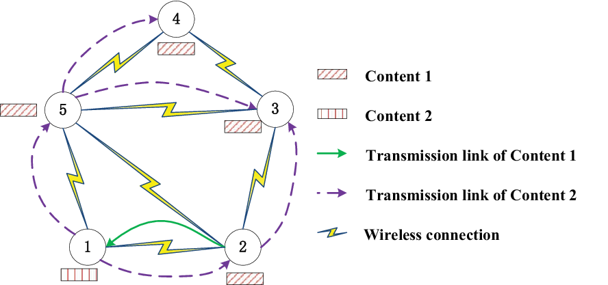
To accurately characterize the NTL distribution in CWN, we propose to define efficient betweenness (EB), which indicates the ratio of content delivery paths passing through a node. Specifically, EB of node is given by
| (2) |
In (2), is the ratio of the number of paths delivering content passing through node to the total number of paths delivering content . Moreover, is denoted as the requested probability of content . According to (2), it is shown that the EB is proposed to capture the impact of content delivery processes among nodes rather than all paths among nodes on NTL distribution. In the example in Fig. 1, we set the probability of each node generating a content request as , , , , and . Since content 2 could be delivered from node 1 to node 3 by two content delivery paths and one path passes through node 5, the average number of paths delivering content 2 from node 1 to node 3 passing through node 5 equals . Similarly, the number of paths delivering content 2 from node 1 to node 4 passing through node 5 equals . Therefore, we have . Moreover, there is no path delivering content 1 passing through node 5. Hence, EB of node 5 is . Similarly, we can obtain that , , , and . To verify the accuracy of EB in quantifying NTL distribution, we provide simulation results of NTL distribution in Fig. 2. Compared with the betweenness based approach, it is obvious that the NTL distribution obtained through the EB based approach is consistent with the real NTL distribution.
In this work, we propose an EB based content caching and delivery strategy to improve throughput capacity in CWN. We formulate an optimization problem to maximize the throughput capacity. Aided by the EB based approach, the throughput capacity is shown to be upper bounded by the minimum ratio of successful delivery probability (SDP) to EB among all nodes. In particular, the throughput capacity is greatly degraded supposing that low-SDP nodes have greater EB, which may consequently result in network congestion. Therefore, we jointly design the content caching and delivery to match an appropriate EB to the SDP of each node. Due to the non-convexity of the primal problem, we solve it by semidefinite relaxation and convex-concave procedure method. Numerical results show that the gap between the proposed strategy and the optimal one (obtained through exhausted search) is kept smaller than 6% and throughput capacity is improved by 60% against the betweenness based strategy under strong interference. Moreover, the computation complexity is shown to be significantly reduced by the proposed algorithm, compared to the optimal one.

II System Model
II-A Network Model
We consider a wireless network consisting of nodes in a two-dimensional plane. The set of nodes is denoted by . We use Voronoi Tessellation to divide the plane into small areas [3]. Nodes located in adjacent areas can deliver contents directly. Let denote the set of contents. We assume that each content is of equal size, which is normalized to one unit, and each node can at most cache contents. Denote as the requested probability of content , which follows the Zipf distribution with parameter [3]. Particularly, the requested probability of content is given by
| (3) |
where a large means that a few contents are requested by majority of nodes. Moreover, we assume that all nodes share subcarriers and each node randomly and independently occupies at most one subcarrier. One node can successfully receive contents when received signal-to-interference-noise-ratio (SINR) is greater than the predefined SINR threshold [4].
In this work, we define the throughput capacity by following the definition in [5].
Definition 1 (Throughput Capacity).
For a given channel scheduling, a throughput of contents per unit time for node is feasible if node can receive contents requested by itself per unit time on average. In this context, the throughput capacity of network is defined as .
II-B Content Transmission Model
We consider that each node has a first-in-first-out transmission queue with limited buffer size. Each content will be deleted from transmission queues until it is successfully received by the next-hop node. Let denote the transmission rate of each node, which is defined as the maximal rate of transmitting contents by nodes. If the received SINR is greater than the predefined SINR threshold, nodes can transmit contents with the transmission rate. Moreover, contents are allowed to be delivered among nodes via multi-hop paths and minimum-hop routing is applied as the routing strategy in the CWN. If there are many minimum-hop paths, the router will randomly choose one for each content.
III Throughput Capacity Maximization
III-A NTL Distribution in CWN
In the following, we propose an EB based approach to quantify the NTL distribution in CWN.
Let denote whether content is cached in node or not, where indicates that node caches content and otherwise. The number of contents cached in each node should not be greater than and each content should be cached once at least in the network11 1 Note that we could first choose a subset of contents to cache in the network if , where the size of the subset is not larger than . The difference of content subset does not influence the analysis and proposed algorithm in the following.. Hence, we have
| (4) |
| (5) |
| (6) |
Meanwhile, we define a binary variable , where indicates that node requests content from node and otherwise. Moreover, we assume that node requests content from only one of nodes caching content and accordingly we have,
| (7) |
| (8) |
Therefore, in definition (2) can be written as
| (9) |
In (9), since each content request will activate a path to delivery the requested content, is equivalent to the average number of paths delivering content to node over seconds. Hence, is the total number of paths delivering content over seconds. Moreover, is the probability that paths delivering content from node to node pass through node . Thus, is the average number of paths passing through node and delivering content to node over seconds. Therefore, is the average number of paths delivering content through node over seconds. Moreover, we can define the average length of all content delivery paths as
| (10) |
where is the number of hops of the minimum-hop path between node and node . In (10), is the total number of paths delivering content over seconds. Moreover, is the length of the path delivering content to node , and is the number of times that node requests content over second. Hence, is the total length of all paths delivering content over seconds. Furthermore, since node can request content from node only if node caches content , and should satisfy
| (11) |
III-B Throughput Capacity
Denote as the total number of contents delivered to next-hop nodes per unit time in the network. We first focus on the process that node delivers content to node . Denote as the node sequence of the minimum-hop path from node to node , where and . If node requests content from node , the average number of content put into the transmission queue of node per unit time equals . When the network goes into the steady state, the number of contents put into the transmission queue of each node should equals the number of delivered by this node. Hence, the average number of content delivered from node to node per unit time should be equivalent to . Similarly, for , the average number of content delivered from node to node per unit time should be equivalent to . Therefore, the total number of content delivered by all nodes in this path to their next-hop nodes per unit time equals . Then, for all processes of content delivering, we can obtain by summing over , , and
Moreover, since contents are delivered along the content delivery paths from the source to the destination, the ratio of contents passing through a node equals the ratio of content delivery paths passing through a node, i.e., EB of this node. Hence, the probability that contents will pass through a node equals the normalized EB of this node, i.e., for node , which is also verified in Fig. 2. Therefore, the number of contents that are put into the transmission queue of node per unit time is given by
| (12) |
We assume that there are minimum-hop paths from node to node . Denote as the node sequence of the -th minimum-hop path, where denotes the -th node in the -th minimum-hop path. Then, we have
| (13) |
Therefore, the sum of all nodes’ EB can be written as
| (14) |
Substituting (14) into (12), we can obtain . Moreover, the number of contents that node can deliver successfully per unit time is , where is the successful delivery probability (SDP) of node . and should satisfy if there is no local congestion in node . Hence, if no congestion occurs in any node in the network, should satisfy
| (15) |
In this work, we consider the case that each node has the same probability of generating a content request per unit time, namely, . In this case, (15) can be rewritten as
| (16) |
According to the Definition 1, the throughput capacity of network equals . According to (16), we can obtain that the upper bound of throughput capacity is under given network parameters. Therefore, we could match the NTL distribution with SDP to maximize throughput capacity.
III-C EB Based Strategy
In the following, we elaborate the detail of the EB based content caching and delivery strategy (ECCDS).
Firstly, we formulate the following optimization problem
To solve the problem (P0), we introduce a new variate , which satisfies constraint (17)
| (17) |
Hence, problem (P0) can be transformed into (P1)
The problem (P1) is an integer linear programming problem. Semidefinite relaxation (SDR) approach [6] can be applied to solve (P1). Aided by SDR, the following relaxed problem can be obtained,
| (18) |
where and , with and . Moreover, in , is a standard unit vector with the -th entry being 1 and with . (P2) is a convex programming which can be solved by using the convex optimization toolbox, such as CVX [7]. After obtaining an optimal solution to the problem (P2), we can generate a series of random vectors as recovery samples. Then, we consider the penalty convex-concave procedure (CCP) method to map each of these recovery samples to the feasible set of problem (P1)[8]. In each iteration, we first define an initial vector , which is one of the samples above. Then, the problem (P2) can be transformed into (P3)
| (19) | ||||
| (20) | ||||
| (21) |
where with , , and . We substitute into (P3). After obtaining the solution , let and increase the penalty factor . Substitute iteratively and into (P3) until stopping criterion is satisfied. The algorithm of penalty CCP method is written in Algorithm 1.
Computation complexity analysis
The proposed algorithm contains two parts, namely, the SDR algorithm and the penalty CCP algorithm. The computation complexity of the two algorithms are studied in the following. (1) The SDR relaxed problem of problem (P1) can be solved by the interior-point algorithm with a worst case complexity of given a solution accuracy [9]. Specifically, is the number of variables in problem (P1) and is the number of constrains in problem (P1). Furthermore, the SDR complexity scales slowly (logarithmically) with . (2) problem (P3) can be solved by the interior-point algorithm with a worst case complexity of [10]. Therefore, the computational complexity of the penalty CCP algorithm is . Specifically, is the number of recovery samples and is the number of iteration for each recovery sample. Therefore, the computational complexity of the proposed algorithm is . For comparison, we also give the computational complexity of the optimal approach, e.g., branch and bound (B&B) method. The worst case of B&B is that each device tries all the possible set of content to cache and tries all the possible set of device to request. The computational complexity of content caching process is . Similarly, the computational complexity of content caching process is . Therefore, the computational complexity of B&B method is . Comparing with the optimal approach, the proposed algorithm can simplify the computation complexity from a power function of the problem size and the number of constraints to a polynomial function. Therefore, the proposed algorithm is a computationally efficient approximation approach to solve problem (P1).
IV Simulation Results
In this section, the simulation results are given. We consider that the number of nodes and contents both equal 10 (, ). All nodes are independently located within an area of the 100100 square meters according to uniform distribution. Moreover, it is assumed that each content is of identical size and, for simplicity, the content size is set to be 1. Note that the results and proposed strategy could be readily applied and extended supposing that the contents are of different size, since they could partitioned into chunks of the identical size [11]. We consider the transmission power of nodes as . The pathloss exponent and noise coefficient are set as and , respectively.
Fig. 3a shows the performance gap between analysis and simulation for two strategies, i.e., ECCDS and uniform caching strategy (UCS). Specifically, in UCS, each node caches each content with same probability. We can observe that simulation results match well with analysis results, thus validating our analysis. Moreover, in Table I, we give simulation results of throughput capacity under different the number of subcarriers . We set the node’s transmission rate , the SINR threshold , and caching storage . We can observe that the value of equals a constant under different . In other words, the throughput capacity is .
| Throughput capacity | |||
|---|---|---|---|
| 2 | 20.1322 | 10.0651 | 2.0002 |
| 4 | 32.0327 | 16.0172 | 1.9999 |
| 6 | 38.1624 | 19.0850 | 1.9996 |
| 8 | 41.7641 | 20.8790 | 2.0003 |
| 10 | 45.8914 | 22.9446 | 2.0001 |


We then compare ECCDS with the BRR-CVR strategy [12]. BRR-CVR strategy is a betweenness based caching strategy, where the popular contents are cached in nodes with high betweenness. We plot throughput capacity as a function of the number of subcarriers in Fig. 3b. For the BRR-CVR strategy, since betweenness can not exactly quantify the NTL distribution in CWN, low-SDP nodes may have high EB, which results in congestion and further degrades the throughput capacity. Moreover, we also provide the throughput capacity of the strategy without matching EB with SDP. The results validates the necessity of matching nodes’ EB with their SDP.
V Conclusion
In this work, we investigate the content caching and delivery strategy to improve throughput capacity of CWN. We define an efficient metric, i.e., EB, to quantify the NTL distribution in CWN. Aided by the EB based approach, we derive that the throughput capacity is upper bounded by the minimum ratio of SDP to EB among all nodes. To maximize the throughput capacity, we design the ECCDS to match an appropriate EB for the SDP of each node. The simulation results show that, particularly under strong interference, the ECCDS can efficiently improve the throughput capacity.
References
- [1] W. X. Wang, Z. X. Wu, R. Jiang, G. Chen, and Y. C. Lai, “Abrupt transition to complete congestion on complex networks and control,” Chaos, vol. 19, no. 3, p. 824, 2009.
- [2] S. Boccaletti, V. Latora, Y. Moreno, M. Chavez, and D. . U. Hwang, “Complex networks: Structure and dynamics,” PHYS REP, vol. 424, no. 4-5, pp. 175–308, Feb. 2006.
- [3] M. Mirahsan, R. Schoenen, and H. Yanikomeroglu, “HetHetNets: Heterogeneous traffic distribution in heterogeneous wireless cellular networks,” IEEE J. Select. Areas Commun., vol. 33, no. 10, pp. 2252–2265, Oct. 2015.
- [4] J. Liu, M. Sheng, L. Liu, and J. Li, “Performance of small cell networks under multislope bounded pathloss model: From sparse to ultradense deployment,” IEEE Trans. Veh. Technol., vol. 67, no. 11, pp. 11 022–11 034, Nov. 2018.
- [5] P. Gupta and P. R. Kumar, “The capacity of wireless networks,” IEEE Trans. Inform. Theory, vol. 46, no. 2, pp. 388–404, 2000.
- [6] Z. Q. Luo, W. K. Ma, M. C. So, Y. Ye, and S. Zhang, “Semidefinite relaxation of quadratic optimization problems,” IEEE Signal Process. Mag., vol. 27, no. 3, pp. 20–34, 2010.
- [7] M. Grant and S. Boyd, “CVX: Matlab software for disciplined convex programming, version 2.1,” http://cvxr.com/cvx, Mar. 2014.
- [8] T. Lipp and S. Boyd, “Variations and extension of the convex-concave procedure,” Optim. Eng., vol. 17, no. 2, pp. 263–287, 2016.
- [9] Z. Luo, W. Ma, A. M. So, Y. Ye, and S. Zhang, “Semidefinite relaxation of quadratic optimization problems,” IEEE Signal Process. Mag., vol. 27, no. 3, pp. 20–34, 2010.
- [10] C. Qian, N. D. Sidiropoulos, K. Huang, L. Huang, and H. C. So, “Phase retrieval using feasible point pursuit: Algorithms and cramer–rao bound,” IEEE Trans. Signal Process., vol. 64, no. 20, pp. 5282–5296, 2016.
- [11] Z. Qin, X. Gan, L. Fu, X. Di, J. Tian, and X. Wang, “Content delivery in cache-enabled wireless evolving social networks,” IEEE Trans. Wireless Commun., vol. 17, no. 10, pp. 6749–6761, 2018.
- [12] B. Chen, L. Liu, Z. Zhang, W. Yang, and H. Ma, “Brr-cvr: A collaborative caching strategy for information-centric wireless sensor networks,” in Proc. IEEE 12th Int. Conf. Mobile Ad-Hoc Sensor Netw. (MSN), 2016, pp. 31–38.